O R I G I N A L A R T I C L E
Open Access
Invisible transportation infrastructure
technology to mitigate energy and
environment
Md. Faruque Hossain
1,2Abstract
Background:Traditional transportation infrastructure built by heat trapping products and the transportation vehiles run by fossil fuel, both causing deadly climate change. Thus, a new technology of invisibleFlying Transportation system has been proposed to mitigate energy and environmental crisis caused by traditional infrastructure system.
Methods:UndergroundMaglevsystem has been modeled to be constructed for all transportation systems to run the vehicle smoothly just over two feet over the earth surface by propulsive and impulsive force at flying stage. A wind energy modeling has also been added to meet the vehicle’s energy demand when it runs on a non-maglev area. Naturally, all maglev infrastructures network to be covered by evergreen herb except pedestrian walkways to absorb CO2, ambient heat, and moisture (vapor) from the surrounding environment to make it cool.
Results:The research revealed that the vehicle will not require any energy since it will run by superconducting electromagnetic force while it runs on a maglev infrastructure area and directed by wind energy while it runs on non-maglev area.
Conclusions:The proposed maglev transportation infrastructure technology will indeed be an innovative discovery in modern engineering science which will reduce fossil fuel energy consumption and climate change dramatically.
Keywords:Maglev technology, Flying transportation, Wind energy for vehicle, Cost reduction, Transportation innovation
Background
Urban and sub-urban area massively depends on trans-portation infrastructure networks which are primarily constructional with concrete and asphalt, and it does not have enough vegetation to absorb heat caused by these asphalt and concrete [1]. Recent research found that transportation infrastructure on earth is appro-ximately 0.9% of the total planetary surface area of 196.9 million mi2 which is equivalent to 1.77 million mi2 infrastructure on earth which causes nearly 6% of global warming by reflecting heat (albedo) back to the space [2, 3]. On the other hand, conventional energy utilization for the transportation sectors is not only costly but also causing adverse environmental impact [4, 5]. A variety of studies have been performed to
understand long-term climate variations by conven-tional energy utilization by the transportation sectors that is casing nearly 28% of global energy consumption which is equivalent to mega ton CO2and is responsible for 28% percent of global warming, and thus infrastruc-ture and transportation fuel cases total 34% global warming [6, 7]. In order to mitigate transportation in-frastructure crisis and its adverse environmental im-pact, I, therefore, propose a new technology of maglev transportation infrastructure system for building better transportation infrastructure system.
A recent study by Cai and Chen described the dy-namic characteristics, magnetic suspension systems, ve-hicle stability, and suspension control laws of maglev/ guideway coupling systems about the maglev transporta-tion system [8, 9], but that fact commercial applicatransporta-tion of this research modeling considering life cycle cost ana-lysis, technology implementation and infrastructure de-velopment did not show the any possibility to apply it
Correspondence:[email protected]
1Green Globe Technology, 4323 Colden Street, Suite 15L, Flushing, NY 11355,
USA
2Department of Civil and Urban Engineering, New York University, 6 Metro
Tech Center, Brooklyn, NY 11201, USA
commercially [1, 10]. Therefore, the approach of this research is to apply the maglev transportation infra-structure commercially for confirming a greener and cleaner transportation infrastructure system where all vehicles shall run just over 2 ft above the earth surface at flying stage by the act of propulsive and impulsive superconducting force. Since the vehicle will run by electromagnetic force, it will not require any energy while running over the maglev. To miti-gate energy consumption when the vehicle needs to run on a maglev area, additional technology has also been proposed to implement wind energy into the vehicle while it is in motion as a backup energy source. Thus, a detailed mathematical modeling using Matlab Simulink software has been implemented for this wind energy utilization for the vehicles by performing turbine and drivetrain modeling [11–13]. A concerted research effort has been performed re-cently on climate science and found that currently 400 ppm CO2 is present in the atmosphere causing global warming, which required to cut down 300 ppm CO2 to confirm global cooling at comfortable stage [14–16]. Once maglev transportation infrastructure system is implemented throughout the world, it will reduce 34% of CO2 per year. Thus, it will take only
R402
300ð1−0:34Þdx
n o
¼66 years to cool the atmosphere, resulting no more climate change after 66 years. Sim-ply, it will be the most innovative technology in mod-ern science to mitigate the cost and global warming dramatically.
Simulations and methods
In order to present maglev transportation infrastructure modeling, I have formulated the following calculation by using Matlab software in terms of (1) guideway model system by adopting Bernoulli-Euler beam equation of series of simply supported beams; (2) Calculation of
magnetic forces for uplift levitation and lateral guidance with allowable levitation and guidance distance consider-ing lateral vibration control LQR algorithm, tunconsider-ing pa-rameters, and Maglev Dynamics.
Guideway model
To prepare the guideway modeling considering free body diagram (Fig. 1), I have considered multiple mag-nets with equal intervals (d) that is to be traveling at a various level speeds of speedv, wherem= beam weight, c = damping coefficient, EIy = flexural rigidity in the y
direction, EIz= flexural rigidity in thezdirection,l= car
length,mw = lumped mass of magnetic wheel,mv= dis-tributed mass of the rigid car body, and θi¼x;y;z ¼ mid-point rotation components of the rigid car body. Considering these, I have formulated the equations of motion for the jth guideway girder carrying a moving maglev vehicle suspended by multiple magnetic forces as follows:
mu::y;jþcyu:y;jþEIyu}}y;j¼ XK
k¼1 Gy;k ik; ;hy;k
φjðxk;tÞ
h i
ð1Þ
mu::z;jþczu:z;jþEIzu}}z;j¼p0−
XK
k¼1 Gz;k ik; ;hz;k
φjðxk;tÞ
h i
ð2Þ
and
φjðxk;tÞ ¼δðx−xkÞ H t−tk− j−1
ð ÞL
v
−H t−tk− jL
v
ð3Þ
together with the following boundary conditions with
lateral (ydirection) support movements:
uy;jð0;tÞ ¼uyj0ð Þt ;uy;jðL;tÞ ¼uyjLð Þt ; EIzuz;j}ð0;tÞ ¼EIzuz;j}ðL;tÞ ¼0
ð4Þ
uz;jð0;tÞ ¼uz;jðL;tÞ ¼0 ð5Þ
EIyu}y;jð0;tÞ ¼EIyu}y;jðL;tÞ ¼0
where (●)′=∂(●)/∂x, (●) =∂(●)/∂t, uz,j(x, t) = vertical
deflection of the jth span, uy,j(x, t) = lateral
deflec-tion of the jth span, L = span length, K = number of magnets attached to the rigid levitation frame, δ (●) = Dirac’s delta function, H(t) = unit step function, k = 1, 2, 3, …, Kth moving magnetic wheel on the beam, tk = (k−1)d/v = arrival time of the kth mag-netic wheel into the beam, xk = position of the kth magnetic wheel on the guideway, and (Gy,k, Gz,k) =
lateral guidance and uplift levitation forces of the kth lumped magnet in the vertical and lateral directions [17, 18].
Magnetic forces of uplift levitation and lateral guidance
Since the maglev vehicle will run over guideway by superconducting force with lateral ground motion (as shown in Fig. 1), guidance forces tuned by the mag-lev system need to be controlled by the lateral mo-tion of the moving maglev vehicle. Therefore, this study adopts the lateral guidance force (Gy,k) and the
uplift levitation force (Gz,k) [19, 20] to keep and
guide the kth magnet of the vehicle, those could be expressed as:
Gy;k¼K0 ikð Þt
hz;k tð Þ
2
Kk;z ð6Þ
Gy;k¼K0 ikð Þt
hz;k tð Þ
2
1−Ky;k
ð7Þ
whereKy,kandKz,krepresent induced guidance factors,
and they are given by:
Ky;k¼
Xkx hy;k
Wð1þXkÞ;
Kz;k¼
Xkx hy;k
Wð1þXkÞ ð
8Þ
In Eqs. (6) and (7),K0=µ0N02A0/4 = coupling factor,
χk =π hy,k/4hz,k, W = pole width, µ0= vacuum perme-ability, No = number of turns of the magnet windings, Ao = pole face area,in(t) =i0+ιn(t) = electric current,
ιn (t) = deviation of current, and (i0, hy0, hz0) = desired
current and air gaps around a specified nominal operat-ing point of the maglev wheels at static equilibrium.
And the uplift levitation (hy,k) and lateral guidance (hz,k)
gaps are respectively given by:
hy;kð Þ ¼t hy0þul;kð Þ−t uy;jð Þxk ;ul;kð Þ ¼t ulcð Þ þt dkθz ð9Þ
hz;kð Þ ¼t hz0þuv;kð Þ−t uz;jð Þ þxk r xð Þk ;uv;kð Þ ¼t uvcð Þ þt dkθy
ð10Þ
where (ul,k, uv,k) = displacements of the kth magnetic
wheel in theyandzdirections, (ulc, uvc) = midpoint
dis-placements of the rigid car, (θy,θz) = midpoint rotations of the rigid car,r(x) = irregularity of guideway, and dk= location of the kth magnetic wheel to the midpoint of the rigid beam. As indicated in Eqs. (6)–(8), the motion-dependent nature and guidance factors (Ky,k,Kz,k) dom-inate the control forces of the maglev vehicle-guideway system. Next, the equations of motion of the 4-DOFs tigid maglev vehicle (see Fig. 1) are written as:
M0u::lc¼g tð Þ þ XK
k¼1Gy;k; ITθ
::
Z¼g tð Þxlþ XK
k¼1 Gy;kdk
ð11Þ
M0u::vc¼p0þ
XK
k¼1Gz;k; ITθ
::
y¼− XK
k¼1 Gz;kdk
ð12Þ
in whichM0=mvl + Kmw= lumped mass of the vehicle, g(t) = control force to tune the lateral response of the maglev vehicle,IT= total mass moment of inertia of the
rigid car, andp0=M0g= lumped weight of the maglev vehicle.
Wind energy modeling for the vehicles
Though the vehicle will run by electromagnetic force, a wind turbine generator is to be used for powering ve-hicle as the additional source of energy to exit veve-hicle from road and park where maglev system is not avail-able. Thus, the model is developed by doubly fed induc-tion generator (DFIG) for producing electricity for transportation vehicles [21]. The fundamental equation governing the mechanical power of the wind turbine is
Pw¼
1
2Cpðλ;βÞρAV
3 ð13Þ
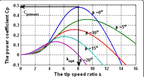
whereρis the air density (kg/m3),Cpis the power
coeffi-cient, Ais the intercepting area of the rotor blades (m2),
Vis the average wind speed (m/s), andλis the tip speed
ratio [16]. The theoretical maximum value of the power
coefficientCpis 0.593; Cpis also known as Betz’s
λ¼Rω
V ð14Þ
whereRis the radius of the turbine (m),ωis the angular speed (rad/s), and V is the average wind speed (m/s). The energy generated by wind can be obtained by
Qw¼PðTimeÞ½kWh ð15Þ
It is well known that wind velocity cannot be ob-tained by a direct measurement from any particular motion [22, 23]. In data taken from any reference, the motion needs to be determined for that particular motion; then, the velocity needs to be measured at a lower motion.
v zð Þln zr zo ¼
v zð Þr ln
z
z0 ð
16Þ
where Zr is the reference height (m), Z is the height at
which the wind speed is to be determined, Z0 is the
measure of surface roughness (0.1–0.25 for crop land),
v(z) is the wind speed at height z (m/s), andv(zr) is the
wind speed at the reference height z (m/s). The power
output in terms of the wind speed shall be estimated using the following equation:
Pwð Þ ¼v
vk−vk C
vk R−vkC
⋅PR vC≤v≤vR
PR vR≤v≤vF
0 v≤vCandv≥vF
8 > > > < > > > :
ð17Þ
wherePRis rated power,vCis the cut-in wind speed,vR
is the rated wind speed, vF is the rated cut-out speed,
and k is the Weibull shape factor [24]. When the blade
pitch angle is zero, the power coefficient is maximized
for an optimal TSR [2]. The optimal rotor speed is to be
calculated by
ωopt ¼λopt
R Vwn ð18Þ
which will give
Vwn¼
Rωopt
λopt ð19Þ
where ωopt is the optimal rotor angular speed in rad/s,
λopt is the optimal tip speed ratio, Ris the radius of the
turbine in meters, andVwnis the wind speed in m/s.
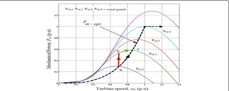
The turbine speed and mechanical powers are depicted in the following graph (Fig. 2), with increasing and decreasing rates of wind speed while the vehicle is in motion [25, 26]. When the wind is steady, the persist-ence forecasts yield good results [27, 28]. When the wind speed is increased rapidly, sudden “ramps” in power output are generated, which is a tremendous benefit for capturing the energy.
Wind energy storage in battery system
Standard Simulink/Sim Power Systems has been calcu-lated by using Matlab-Simulink for the wind energy con-version that is to be stored in circuit-implemented inverter as a storage buffer, and all the electricity is to be supplied through the battery according to Peukert’s law to start the engine and to be used when the vehicle is not in motion [19, 24, 29].
Design of traffic control
Though underground maglev system has the capability to allow run up to 580 kph, the vehicles’high speed shall be calculated based on traffic flow, composition, volume,
number and location of access points, and local environ-ment importantly allotting sufficient number of lanes considering Greenshield’s following road and highway capacity analysis (Fig. 3).
Since the maglev technology is invisible, thus, to alert the drivers and pedestrian, the maglev roads, highways, and its exits should be constructed by landscaping by covering the guideway by herb (green grass) and in be-tween lanes at least two feet to be left blank (no land-scaping) in order to differentiate the lanes.
Results and discussion
Based on the mathematical modeling described above, I have performed load resistant factor design (LRFD) cal-culation considering the following equation and selected W24 × 84 beam which is the continuous maglev under-ground runs (metal track guideway) that need to be structurally sound to carry enough current, load, and levitate force of the vehicles.
Fy∝nl 2
h ð20Þ
Fx∝ −1 ktvx Fx∝
−nl2
h ð21Þ
where Fy is the vehicle weight,nis the total number of coils in maglev, l is the current on each coil, h is the height of levitation, t is the thickness of conduction track, andkis the conductivity of track.
To construct under maglev guideway just 2 ft below of the earth surface, it will need to have a U-shaped cross-section to fix the pole position [30]. Naturally, heavy duty waterproofing membrane is to be used to protect
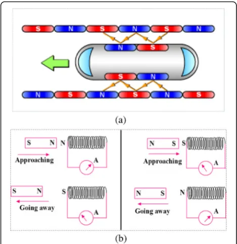
the maglev underground runs for avoiding floods and moisture. It is well researched that the propulsion coils run in elliptical loops along both walls of the guideway, generating magnetic force when electricity runs through them [4]. So, levitation and guidance coils that will be formed will create their own magnetic force once the ap-plied superconducting magnets pass on it, where propul-sion and levitation are the key factor to run the vehicle. In propulsion, as the direction of the current charges back and forth in the propulsion coils above the wall of the guideway, the north and south poles will reserve re-peatedly and shall propel the vehicle by alternating force of attracting and repulsion (Fig. 4). In levitation, as the vehicle passes, an electric current is induced in the coil along the guideway and the vehicle will be levitated by the force of attraction, which will pull up on the magnet in the vehicle, as well as by repulsion, which will push up on the magnet [31].
To create levitation and lateral balance in the vehicle, an electromagnetic induction is to be used. To confirm the most efficient and economical way to produce a powerful magnetic field by using the superconducting coils, I have assumed the permanent currents of about 700,000 A go through these superconducting coils [31], hence creating a strong magnetic field of almost 5 T, i.e., 100,000 times stronger than the earth’s magnetic field by implementing the following block diagram (Fig. 5).
Simply, it can be explained that when an electric current flows through the propulsion coils, a magnetic field is produced. The forces of attraction and repulsion between the coils and the superconducting magnets on the vehicle propel the vehicle forward in a flying stage up to 4 ft height where 2 ft shall be considered under-ground cover and the other 2 ft is just over the earth surface (Fig. 6). The vehicle’s speed is to be adjusted by altering the timing of the polarity shift in the propulsion
Speed Increasing
Optimum Speed (Vm)
Speed Decreasing
Km Density
(k) 0
qm
Flow (q)
Speed (v) Vm vf
Flow (q)
qm
0 0 Km
Density (k)
kj Speed
(v) Vm vf
(a)
(b)
(c)
coils’ magnetic field between north and south with the possibility of maximum speed of 580 kph [31]. As the vehicle passes just 2 ft above the guideway (1 ft from the earth surface), an electric current is induced in the levi-tation and guidance coils, creating opposite magnetic poles in the upper and lower loops. The upper loops be-come the polar opposite of the vehicle’s magnets,
producing attraction, which pulls the vehicle up. The lower loops have the same pole as the magnets. This generates repulsion, which pushes the vehicle in the same direction up. The two forces combine to levitate the vehicle, while maintaining its lateral balance between the walls of the guideway.
Subsequently, a niobium-titanium alloy is to be used to create superconducting magnets for maglev, but to reach superconductivity, they must be kept cold. In order to keep the alloy cool, liquid helium should be used with a temperature of −269 °C since alloy retains superconductivity at temperatures up to−263 °C, though the maglev system can operate better at 6 °C to produce sufficient magnetic force.
In addition to underground maglev construction, the wind turbine generation system is to be installed on ve-hicles as the the backup energy source by the oper-ational performace of wind turbine while vehicle is in a motion.
These conditions permit application of the wind pro-file which is considered to be a wind speed signal with a mean value of 8 m/s and a rated wind speed of 10 m/s; the whole system is tested under standard conditions with a stator voltage of approximately 50% for 0.5 s be-tween 4 and 4.5 s, approximately 25% bebe-tween 6 and 6.5 s, and 50% between 8 and 8.5 s (Fig. 7). Thus, the machine is considered to be functioning in ideal condi-tions (no perturbacondi-tions and no parameter variacondi-tions). Moreover, to guarantee a unity power factor at the stator side, the reference for the reactive power is to be set to zero [32]. As a result of increasing wind speed, the gen-erator shaft speed achieved maximum angular speed by tracking the maximum power point speed. Thus, the wind turbine always works optimally since the pole placement technique is to be used to design the tracking
Fig. 4The above figures indicate the polarization of the coil in different cases:aSchematic diagram of the director of the running vehicle (must be construction with magnet as shown on this diagram) on maglev propulsion via propulsion coils.bNear the receding S-pole, becomes an N-pole to oppose the going away of the bar magnet’s S-pole
Fig. 5Block diagram to control the mathematically modeled magnetic bearing system, a process to design the driver to operate the
control [15]. Consequently, decoupling among the com-ponents of the rotor current was also performed to con-firm that the control system worked effectively. The bidirectional active and reactive power transfer between the rotor and power system is exchanged by the gener-ator according to the super synchronous operation, achieving the nominal stator power, and the reactive power can be controlled by the load side converter to obtain the unit’s power factor to generate energy for powering vehicles [6, 14].
Construction cost estimate comparison
Order of magnitude cost estimate was performed by using HCSS (Heavy Bid) software standard union rate of New York State locals with a project of 10% general con-dition, 10% overhead and profit, and 3% contingency over the hard cost of labor, materials, and equipment comparing between maglev infrastructure and trad-ition infrastructure system for a sample of 100 miles long and 128 ft wide (12 ft wide of four lanes on each directions, two-sided 10 ft service space, and
6 ft median in the center of the road). In order to determine that the underground guideway (w24 × 84) can last long, I have calculated again the LRFD to provide the shoring of both sides for the entire 100 miles long and 128 ft wide (12 ft wide of 4 lane each directions two sided 10 ft service space and 6 ft median in the center of the road) construction cost considering standard excavation up to 6 ft deep, with appropriate shoring with minimum embedment depth L4 is 5 ft and standard soil pressure ϒs = 120 lbf/ft3, angle of pressure Φ = 210, and the soil pressure coef-ficient c = 800 lbf/ft2. To prepare the conceptual esti-mate, we need to determine the length of soldier piles. I have counted 6′ OC (on center) soldier piles at both sides by illustrating and using the following LRFD method that soldier piles must be set at to support the necessary excavation and/or earth pres-sure against collapse.
Active Earth Pressure Ka¼tan2 45o−Φ
2
ð22Þ
Passive Earth Pressure Kb¼tan2 45oþΦ
2
ð23Þ
Use Eqs. (22) and (23) to find the lateral earth pressure the solid piles must support.
PEM¼ϒsh ka;piles
¼ 120lbf
ft3 0 @
1
A⋅ð Þ6:0 tan2 45o−21 o 2 0 @
1 A
¼340:128 lbf=ft2
to determine the type of steel beams required for the soldier piles, we have taken the bending moments about the tributary area of the piles.
Soil pile spacing¼6ft
Side elevation
M¼M¼2040:768 ft‐lbf=ft
M¼
340:128 lb
ft2
0 @
1 Að6 ftÞ
2 0
B B B B B B @
1 C C C C C C A
6 ft 3 0 @
1
A ¼2040:768 ft‐lbf=ft
The moment is a distributed moment applied to the base of the tributary area of each soldier pile. Therefore,
Fig. 6The Maglev vehicle’s force and directional diagram as shown by propulsion guidance coils and superconducting coils
the moment is 2040.768 ft-lbf per foot. The total mo-ment on the soldier pile (at the base) is
M0¼Mð6 ftÞ
¼ 2040:768 ft−lbf ft
0 @
1 Að6 ftÞ
¼12;244:61 ft‐lbf
Now,
Zreq¼
M0
Φb Fy¼
12 in
ft
0 @
1
Að12;244:61ft−lbfÞ
0:9
ð Þ 50;000 lbf in2
0 @
1 A
¼3:27 in3
From AISC tables, the soldier piles have been selected as W12 × 26, and the perpendicular support w8 × 12 members 6 ft long.
Then, we have determined the depth required below subgrade by calculating the passive earth pressure coeffi-cient using Eq. (23)
Kp¼tan2 45ÅþΦ
2 0 @ 1 A 0 @
¼tan2 45Åþ21Å
2
0 @
1 A
¼2:12
Then, we have calculated the active earth pressure coefficient using Eq. (22)
Ka¼tan2 45Å−Φ
2
0 @
1 A
¼tan2 45Å−21Å
2
0 @
1 A
¼0:4724
In order to determine the slopes of the excavation, depth is required. Since below the bottom of the excava-tion, both pressure are considered to be passive and have the same slope, the slope of the pressure profile above the reversal point is calculated from the standard equa-tion for the slope, using L3as the rise and ϒhkaas the run (a value equal to the lateral earth pressure, expressed this way for the purposes of cancelation). Thus, the slope of the pressure profile below the reversal point can be calculated similarly, using L4 as the rise
and the product ofϒL4kpas the run. Because the slopes are the same, the two equations can be equated. Re-arranging to solve for L3,
L3
ϒhka¼ L4
ϒL4kp
L3¼ hka
kP ¼
6 ft
ð Þð0:4724Þ 2:12
¼1:337 ft
The necessary embedment depth is 1.337 ft + 5 ft = 6.337 ft
The total required soldier pile length is 6.337 ft + 6 ft = 12.337 ft (13 ft assumed)
So, I have determined that the solder pile (W12 × 26) should be 13 ft long, and the perpendicular support (w8 × 12) should be 6 ft long as the support for structur-ally sound maglev construction.
To construct the long lasting and sophisticated under-ground maglev, I have performed load resistant factor design (LRFD) calculation and selected W24 × 84 beam that the continuous maglev underground runs (struc-tural beam) are struc(struc-turally sound. Then I have calcu-lated the required shoring concept for 100 miles long and 128 ft wide construction cost considering standard excavation up to 6 ft deep, with appropriate shoring with minimum embedment depth. L4 is 5 ft and standard soil pressureϒs= 120 lbf/ft
3
, angle of pressureΦ = 210, and the soil pressure coefficient c = 800 lbf/ft2 in order to determine the length of soldier piles. So, I have calcu-lated by using LRFD methods again that selected that the solder pile (W12 × 26) should be 13 ft long, and the perpendicular support (w8 × 12) should be 6 ft long as the support maglev construction.
Cost of maglev infrastructure
The proposed maglev infrastructure, therefore, requires shoring, excavation, structural steel, and concrete oper-ation, and thus I have calculated the estimate consider-ing the followconsider-ing components:
Shoring at 13′deep with w24 × 26 steel soldier piles at 6′OC both side $2/lf; top rail w8 × 12 both sides $2/ lf; 6′length w8 × 12 perpendicular support 20 OC $2.lf; and protection board 1,372,800 ft2 both side at $4/ft2 ,and thus the total cost would be $23,724,800.
Excavation (5,2800’length× 128width× 6deep× 1.3fluff fac-tor)/27 is 19,524,266.67 yd3at $56/yd3 cost for digging, stock piling, and backfilling, and the total cost would be $1,093,358,933.
and the cost is $62,577,778; concrete form at $2/ft2 is $16,896,000, and thus the total cost of material is $528,156,445.
Cost of labor: 200 iron worker for 2704 working days at $100/h; 100 concrete cement workers for 2704 work-ing days at $90/h; 100 laborer for 2704 workwork-ing days at $70/h; 50 equipment operator for 2704 working days at $100/h, and thus the total labor cost is $886,912,000 considering standard 8 h a day.
Equipment cost: 10 small renting at $1000/day; 10 small tool renting at $250/day; 271 concrete pump at $2000/each, and thus the total equipment cost is $34,342,000.
Other cost: engineering service at $5/ft2; survey team at $4400/day for each working days, and thus the total cost is $349,817,600.
The net construction cost by adding 10% general con-dition, 10% overhead and profit, and 3% contingency into the excavation, material, labor, equipment, and other cost would be $$3,587,063,487.
Cost of traditional road infrastructure
A typical highway consists of 8″ asphalt surface course, 4″binder course, 4″base course, and 12″aggregate with standard wiremesh or framing, and thus we have calcu-lated the estimate considering the following components:
Excavation (52,800length × 128width × 2.33deep × 1.3fluff factor)/27 is 7,581,924 yd3 at $56/yd3 cost for digging, stock piling, and backfilling, and the total cost would be $424,587,744.
Cost of materials: $50/yd3; 4″ base course is 834,370 yd3 at $50/yd3; wire-mesh or framing is (528,000 × 128) at $1/ft2, and 12″ subbase aggregate is 2,503,111 yd3at $25/yd3, and thus the total cost of ma-terial is $380,472,775.
Cost of labor: 200 asphalt cement workers for 2704 working days at $100/h; 200 labor foremen for 2704 working days at $100/h; 200 laborers for 2704 working days at $70/h; 200 equipment operators for 2704 work-ing days at $100/h; 100 truck drivers for 2704 workwork-ing days at $100/h; 200 small roller engineers for 2704 work-ing days at $100/h, and thus the total cost is $2,249,728,000.
Equipment cost: 200 roller renting at $1000/week; 200 milling renting at $10,000/week; 100 truck renting at $500/week, and thus the total cost is $502,171,429.
Other cost: detailing and shop drawing at $10/ft2; en-gineering service at $5/ft2; survey team at $4400/day for each working days; banking service of 301,037 yd3 at $1000/yd3; maiden concrete divider is 106,468 yd3 at $818/yd3, and thus the total cost is $1,326,694,600.
The net construction cost by adding 10% general con-dition, 10% overhead and profit, and 3% contingency
into the excavation, material, labor, equipment, and other cost would be $6,805,115,863.
Cost saving
In this article, I have calculated cost saving by using standard 100-mile highway of 128 ft wide (12 ft wide of four lanes on each directions, two-sided 10 ft service space, and 6 ft median in the center of the road) as an experimental tool to compare construction cost in be-tween conventional and maglev infrastructure system. Total cost estimate for traditional infrastructure is $6,805,115,863, and the maglev infrastructure system cost is only $3,587,063,487 for the same 100-mile high-ways and the net cost saving is $3,218,052,377 (Table 1). Consequently, it will reduce neatly 50% of the cost once maglev infrastructure system is used for the construction of invisible infrastructure which is also benign to the environment.
Conclusions
Traditional transportation infrastructure construction throughout the world is not only expensive, but also consumes 5.6 × 10²⁰J/yr (560 EJ/yr) fossil fuel each year which indeed dangerous of a cliché when discussing about climate [33, 34]. To mitigate these problems, bet-ter infrastructure transportation planning is needed to be done where environmental sustainability and climate adaptation are to be confirmed for the creation of com-munities more resilient and vibrant. Interestingly, the Maglev Infrastructure Transportation technology pro-posed in this article, for urban infrastructure transporta-tion system, implicated by electromagnetic and superconducting magnets will, thus, be the emergent technology in modern science to console infrastructure, energy, and environmental dire straits, just because this technology is cheaper and will run by repulsive-force and attractive-force at the levitated (flying) stage while it will run on maglev system and will run by air (wind en-ergy) while it is on non-levitated area without consum-ing fossil fuel. Indeed, this new maglev infrastructure transportation system would be the innovative technol-ogy ever to console infrastructure, transportation, en-ergy, and global warming crisis.
Acknowledgements
This research was supported by Green Globe Technology under support of RD-02017-10. Any findings, conclusions, and recommendations expressed in this paper are solely those of the author and do not necessarily reflect those of Green Globe Technology.
Author’s Information
Dr. Md. Faruque Hossain has over 20 years of experience in research, development, and program management for sustainable technology specialized in energy, environment, building, civil, and infrastructure projects. He worked and/or consulted in diverse small companies to fortune listed companies and managed as less as million dollars to over billion dollar projects. Faruque also worked for New York City as the Director of Technical
Services. He got his Ph.D. from Hokkaido University, did post-graduate re-search in Engineering at the University of Sydney, and Executive Education in Architecture at Harvard University. He is a LEED-certified professional and an editor of several international Journal of Sustainable Technology related field. Dr. Hossain is the president of Green Globe Technology, Inc. and the adjunct professor at New York University at the department of civil and urban engineering.
Competing interests
The author declares that he has no competing interests.
Publisher’s Note
Springer Nature remains neutral with regard to jurisdictional claims in published maps and institutional affiliations.
Received: 23 May 2017 Accepted: 1 August 2017
References
1. Chang S (2003) Evaluating disaster mitigations: methodology for urban infrastructure systems. Nat Hazards Rev 4:4. doi:10.1061/(ASCE)1527-6988 (186), 186–196
2. Pugh TA, MacKenzie AR, Whyatt JD, Hewitt CN (2012) Effectiveness of green infrastructure for improvement of air quality in urban street canyons. Environ Sci Technol 46(14):7692–7699. doi:10.1021/es300826w
3. Werner, Johannes P., Juerg Luterbacher, and Jason E. Smerdon. A Pseudoproxy Evaluation of Bayesian Hierarchical Modelling and Canonical Correlation Analysis for Climate Field Reconstructions over Europe, Journal of Climate, 2012;40(9): 1293–1300
4. Yau JD (2012) Lateral vibration control of a low-speed maglev vehicle in cross winds. Wind Struct 15(3):263–283
5. Mann ME, Bradley RS, Hughes MK (1998) Global-scale temperature patterns and climate forcing over the past six centuries. Nature 392:779–787 6. Liu, Zhu, Dabo Guan et al.“Reduced carbon emission estimates from fossil
fuel combustion and cement production in China”, Nature, 2015
7. O’Neill BC, Oppenheimer M (2004) Climate change impacts sensitive to path to stabilization. Proc Natl Acad Sci 101:16,411–16,416
8. Thompson SJ, Congressional Research Service (1989) High Speed Ground Transportation (HGST). Prospects and Public Policy 6:5
9. Cai Y, Chen SS, Rote DM, Coffey HT (1996) Vehicle/guideway dynamic interaction in maglev systems. J Dyn Syst Meas Control 118:526–530
10. Cai Y, Chen SS (1997) Dynamic characteristics of magnetically-levitated vehicle systems. A Mech Rev 50(11):647–670
11. Chakib R, Essadki A, Cherkaoui M (2014) Modeling and control of a wind system based on a DFIG by sctive disturbance rejection control. International Review on Modelling and Simulations (IREMOS)
12. Jeong S-Y, Nguyen TH, Le QA, Lee D-C (2016) High-performance control of three-phase four-wire DVR systems using feedback linearization. Journal of Power Electronics
13. He, Ping, Fushuan Wen, Gerard Ledwich, and Yusheng Xue. Small signal stability analysis of power systems with high penetration of wind power, Journal of Modern Power Systems and Clean Energy, 2013
14. Hossain MF (2016) Solar energy integration into advanced building design for meeting energy demand and environment problem. Int J Energy Res 15. Werner JP, Luterbacher J, Smerdon JE (2012) A pseudoproxy evaluation of
Bayesian hierarchical modelling and canonical correlation analysis for climate field reconstructions over Europe. J Clim
16. Zheng XJ, Wu JJ, Zhou YH (1997) Numerical analyses on dynamic control of five-degree-of-freedom maglev vehicle moving on flexible guideways. J Sound Vib 235:43–61
17. El-Anwar, Omar, Jin Ye, and Wallied Orabi. Efficient Optimization of Post-Disaster Reconstruction of Transportation Networks, Journal of Computing in Civil Engineering, 2015
18. Elmansouri, A., J El mhamdi, and A. Boualouch. Wind energy conversion system using DFIG controlled by back-stepping and RST controller, 2016 International Conference on Electrical and Information Technologies (ICEIT), 2016 19. Aldo D, Alfred R (1999) Design of an integrated electromagnetic levitation
and guidance system for Swiss Metro, EPE'99. Lausanne, Swiss
21. Khodakarami, Jamal, and Parisa Ghobadi. Urban pollution and solar radiation impacts, Renewable and Sustainable Energy Reviews, 2016
22. Astrom KJ, Hagglund T (1988) Automatic tuning of PID controllers. Instrument Society of America, USA
23. Bhandari B, Poudel SR, Lee K-T, Ahn S-H (2014) Mathematical modeling of hybrid renewable energy system: a review on small hydro- solar-wind power generation. International Journal of Precision Engineering and Manufacturing-Green Technology
24. Zhao CF, Zhai WM (2002) Maglev vehicle/guideway vertical random response and ride quality. Veh Syst Dyn 38(3):185–210
25. Kerrouche, K., A. Mezouar, and L. Boumedien. A simple and efficient maximized power control of DFIG variable speed wind turbine, 3rd International Conference on Systems and Control, 2013
26. Lala H, Karmakar S (2015) Continuous wavelet transform and artificial neural network based fault diagnosis in 52 bus hybrid distributed generation system. IEEE Students Conference on Engineering and Systems (SCES):2015 27. Loucif, Mourad, and Abdelmadjid Boumediene. Modeling and direct power
control for a DFIG under wind speed variation, 2015 3rd International Conference on Control Engineering & Information Technology (CEIT), 2015 28. Lu L (2002) Investigation on wind power potential on Hong Kong islands-an
analysis of wind power and wind turbine characteristics. Renew Energy 09 29. Kamili H, Riffi ME (2016) Portfolio optimization using the Bat algorithm.
International Review on Computers and Software (IRECOS)
30. Chevallier F. On the statistical optimality of CO2atmospheric inversions assimilating CO2column retrievals, Atmos, Chem, Phys., 15, 11133-11145, doi:10.5194/acp-15-11133-2015, 2015
31. Abdelmalek, Samir, Linda Barazane, Abdelkader Larabi, and Hocine Belmili. Contributions to diagnosis and fault tolerant control based on Proportional Integral Observer: Application to a doubly-fed induction generator, 2015 4th International Conference on Electrical Engineering (ICEE), 2015
32. Zheng XJ, Wu JJ, Zhou YH (2005) Effect of spring non-linearity on dynamic stability of a controlled maglev vehicle and its guideway system. J Sound Vib 279:201–215
33. Soong TT (1990) Active structural control: theory and practice. Longman Scientific & Technical, Essex, England