RESEARCH
Generalized enhanced suffix array
construction in external memory
Felipe A. Louza
1, Guilherme P. Telles
2, Steve Hoffmann
3and Cristina D. A. Ciferri
4*Abstract
Background: Suffix arrays, augmented by additional data structures, allow solving efficiently many string processing problems. The external memory construction of the generalized suffix array for a string collection is a fundamental task when the size of the input collection or the data structure exceeds the available internal memory.
Results: In this article we present and analyze eGSA [introduced in CPM (External memory generalized suffix and LCP arrays construction. In: Proceedings of CPM. pp 201–10, 2013)], the first external memory algorithm to construct
generalized suffix arrays augmented with the longest common prefix array for a string collection. Our algorithm relies on a combination of buffers, induced sorting and a heap to avoid direct string comparisons. We performed experi-ments that covered different aspects of our algorithm, including running time, efficiency, external memory access, internal phases and the influence of different optimization strategies. On real datasets of size up to 24 GB and using 2 GB of internal memory, eGSA showed a competitive performance when compared to eSAIS and SAscan, which are efficient algorithms for a single string according to the related literature. We also show the effect of disk caching managed by the operating system on our algorithm.
Conclusions: The proposed algorithm was validated through performance tests using real datasets from different domains, in various combinations, and showed a competitive performance. Our algorithm can also construct the gen-eralized Burrows-Wheeler transform of a string collection with no additional cost except by the output time.
Keywords: Suffix array, LCP array, Burrows–Wheeler transform, External memory algorithms, String collections
© The Author(s) 2017. This article is distributed under the terms of the Creative Commons Attribution 4.0 International License (http://creativecommons.org/licenses/by/4.0/), which permits unrestricted use, distribution, and reproduction in any medium, provided you give appropriate credit to the original author(s) and the source, provide a link to the Creative Commons license, and indicate if changes were made. The Creative Commons Public Domain Dedication waiver (http://creativecommons.org/ publicdomain/zero/1.0/) applies to the data made available in this article, unless otherwise stated.
Introduction
Suffix arrays [40] (also known as PAT arrays [23]) may be used for the solution of string processing problems in several areas, including pattern matching, data compres-sion and information retrieval [24, 39, 47]. Combining a suffix array with the longest common prefix (LCP) array and with the Burrows–Wheeler transform (BWT) [12] provides a data structure, an enhanced suffix array (ESA) [2], that enables solving many string processing problems in optimal time and space.
Using such structures in the solution of problems involving strings is usually done in two steps: the struc-ture is first constructed and then it is queried. This article is about the construction of generalized enhanced suffix
arrays for a collection of strings using external memory. This is motivated by the rising number of applications that deal with huge sets of strings, such as those in Bio-informatics and Internet searching. Moreover, recent advancements in non-volatile storage technologies have substantially narrowed the gap between internal and external memory access times, making the querying of external suffix arrays significantly faster.
Different algorithms have been proposed for internal memory suffix array construction (see [17, 49]), including algorithms with linear running time [30, 33, 46]. Gonnet et al. [23] proposed the first external memory algorithm for constructing suffix arrays. Later, Crauser and Ferra-gina [14] adapted internal memory algorithms to work in external memory. Dementiev et al. [16] observed that these algorithms do not scale well and presented a pipe-lined version of the internal memory algorithm DC3 [30] to external memory. Nong et al. [44, 45] adapted the
Open Access
*Correspondence: [email protected]
4 Institute of Mathematics and Computer Science, University of São Paulo, Av. Trabalhador São-carlense, 400, São Carlos 13560-970, Brazil
internal memory algorithms SA-DS and SA-IS [46] to external memory, and Liu et al. [34] presented an enhanced version of SA-IS to external memory. Kärk-käinen and Kempa [25] presented the SAscan algorithm,
improving on the earlier proposal by Gonnet et al. [23], and later, Kärkkäinen et al. presented a parallel external version of SAscan algorithm [27].
BWT can be either obtained from the suffix array or constructed directly in internal memory in linear time [48]. Ferragina et al. [18] proposed an external memory algorithm to construct the BWT for a single string, and Bauer et al. [5] presented external memory algorithms to compute and decode the BWT for a string collection.
LCP construction in internal memory is also possible in linear time during the suffix array construction [19, 35] or afterwards, given the suffix array [29, 31, 41] or the BWT as input [7, 22]. Kärkkäinen and Kempa [26] pre-sented the LCPscan, an external memory algorithm to
construct LCP arrays given the suffix array as input, and Bauer et al. [6] proposed the extLCP algorithm to
con-struct both BWT and LCP arrays for large collections of equally sized strings in external memory, and later, Cox et al. [13] presented an extended version of extLCP to
deal with strings with different sizes.
The suffix and the LCP arrays are constructed together in external memory by eSAIS, proposed by Bingmann et al. [10], one of the most efficient external memory algorithm to date. There exists alternatives to compute suffix and LCP arrays in parallel [20] and using small space [37, 42].
In this article we present and analyze the algorithm
eGSA (introduced in [38]) in depth. To our
knowl-edge this is the first algorithm to construct generalized enhanced suffix arrays in external memory. We compared
eGSA with the most efficient related algorithms in the
literature, eSAIS [10] and SAscan [25]. Although eSAIS and SAscan can easily be applied to the concatenation
of a string collection, our method is shown to run faster in practice. In addition to the LCP array, our method also constructs the BWT for the collection. eGSA uses a
heap and a combination of optimization procedures that are shown to be very effective in practice. The optimiz-ing strategies that we propose in this article are based on nice properties of strings and their relation with the LCP array, and are applied across the nodes of a heap.
Theoreticallly, eSAIS runs in O(nlog
M/B(n/B)) time
and O((n/B)logM/B(n/B)) I/Os, where n is the length of
the input string, B is the disk block size and M is the RAM size. SAscan runs in O((n2/M)log(2+log
σ/log logn))
time and O(n2logσ/(MBlogn)+(n/B)logM/B(n/B)) I/
Os. Our algorithm runs in O((Nlogm)maxlcp) time and O(Nlogm|Tℓ|) I/Os, where N is the sum of the m string
lengths in the input, maxlcp is the length of the longest
common prefix between suffixes of the input strings, |Tℓ| is the length of the longest string in the collection.
The rest of the article is organized as follows. " Back-ground" section introduces concepts and nota-tion, "eGSA" section describes the algorithm and presents a theoretical analysis, "Performance evaluation" section details the experiments, results and investigates limita-tions of the algorithm. "Conclusions" section concludes the article.
Background
Let be an ordered alphabet of symbols. We denote the
set of every string of symbols in by ∗ and the
con-catenation of strings or symbols by the dot operator (·).
Let $ be a symbol not in that precedes every symbol
in with respect to the alphabetical order. We define $= {T ·$|T ∈∗}. We use the symbol < for the
lexico-graphic order relation between strings.
The ith symbol in a string T of length n is denoted T[i], 1≤i≤n. A substring of T is denoted T[i,j] =T[i] ·. . .·T[j],1≤i≤j≤n. A prefix of T is a
substring of the form T[1, k] and a suffix is a substring of the form T[k, n], 1≤k≤n.
A suffix array for a string T ∈$ of size n, denoted SA, is an array of integers SA= [i1,i2,. . .,in] such that T[i1,n]<T[i2,n]<· · ·<T[in,n]. Thus, a suffix array
provides the lexicographic order for all suffixes of a string. Let pos(T[k,n]) denote the mapping of suffix T[k, n] to its position in SA, i.e. the reverse suffix array, and let suff(j) denote the mapping of position j of SA to the
suf-fix represented at j, namely T[SA[j],n].
Let lcp(S,T) be the length of the longest com-mon prefix of two strings S and T in $. The LCP array for T is an array of integers such that
LCP[i] =lcp(T[SA[i],n],T[SA[i−1],n]) and
LCP[1] =0.
The BWT is a reversible transformation obtained through cyclic rotations of a string, and results in another string that is easier to compress [12]. The BWT has a close relationship to the suffix array and can be trivially obtained from it. Let the BWT of a string T be denoted BWT and defined as BWT[i] =T[SA[i] −1] if SA[i] �=1
or BWT[i] =$ otherwise.
We will refer to the structure formed by SA,LCP,BWT as an enhanced suffix array, denoted ESA [2]. Table 1
shows the enhanced suffix array for T1=GATAGA$ and
for T2=TAGAGA$.
Let T be a collection of m strings {T1,. . .,Tm} from $
having lengths n1,. . .,nm. We extend the lexicographic relation among strings to deal with unit length suffixes of
The generalized suffix array of T, denoted GSA,
is an array of pairs of integers (a, b) that speci-fies the lexicographic order of all suffixes Ta[b,na] of strings in T. We denote the first component of GSA[j] as GSA[j].str∈ [1,m] and the second as GSA[j].suf ∈ [1, max{n1,. . .,nm}]. Also, we extend the
function suff(j) to map the suffix represented at position j of GSA, namely TGSA[j].str[GSA[j].suf,nGSA[j].str].
The generalized LCP of T is defined as
LCP[j] =lcp(suff(j),suff(j−1)) and LCP[1] =0, and the generalized BWT of T is defined as BWT[j] =TGSA[j].str[GSA[j].suf −1] if GSA[j].suf �=1
or BWT[j] =$ otherwise.
The generalized suffix array of T together with its
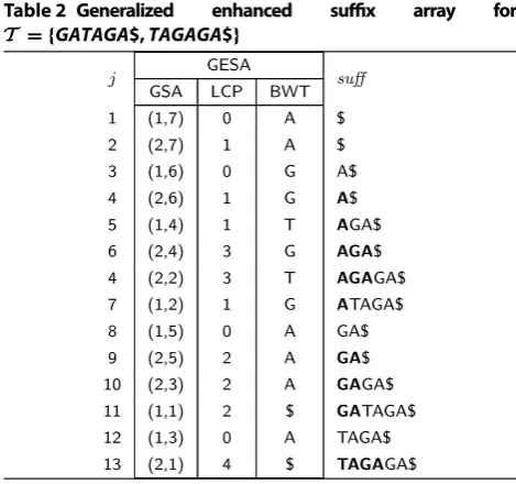
cor-responding LCP array and BWT will be called generalized enhanced suffix array and denoted GESA. Table 2 shows
the generalized enhanced suffix array for T = {T1,T2}, where T1=GATAGA$ and T2=TAGAGA$.
eGSA
The External Generalized Enhanced Suffix Array Con-struction Algorithm (eGSA) resembles a two-phase
multiway merge-sort [32]. Algorithm 1 illustrates eGSA
without the otimizing strategies introduced in Phase 2. Phase 1 builds the enhanced suffix arrays for the input strings and Phase 2 merges the respective arrays using an improved string comparison method on memory buffers. We detail each phase below.
Phase 1: internal sorting
The input for eGSA is a collection T of m strings T = {T1,. . .,Tm} having lengths n1,. . .,nm with total
length N and stored in external memory.
In Phase 1 the suffix array SAi, the LCP array LCPi, the Burrows–Wheeler transform BWTi and the auxiliary array PREFIXi are built for each Ti and stored in external
mem-ory (lines 1–9 of Algorithm 1). Any internal or external memory suffix and LCP array construction algorithm may Table 1 Enhanced suffix arrays for T1=GATAGA$ and for
T2=TAGAGA$
Table 2 Generalized enhanced suffix array for
T = {GATAGA$, TAGAGA$}
be used by eGSA to build SAi and LCPi (line 2). As they are constructed, both BWTi (line 5) and PREFIXi (lines
6) can be computed and written sequentially to external memory with no need to store in internal memory.
PREFIX arrays are used to reduce external memory
accesses in Phase 2: starting from a position j and con-catenating PREFIXi successively for adjacent preceding
positions will render a prefix of Ti[j,ni], up to a position
with lcp equal to zero. In other words, PREFIXi[j] will
store symbols from the string, such that the contents of
PREFIXi[j] concatenated to parts of preceding positions
of PREFIX is equal to a starting portion of the suffix at
position SAi[j]. More formally, let p be a given integer
constant. Let h0=0 and hj=min(LCPi[j],hj−1+p).
We define PREFIXi[j] =Ti[SAi[j] +hj,SAi[j] +hj+p].
As a boundary condition, whenever the length of Ti is
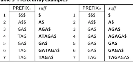
exceeded, sufficient $ symbols are added to the right of PREFIXi[j]. An example for the ESAs from Table 1 with p=3 is shown in Table 3. Notice that it is possible to
recall the strings with the aid of PREFIX. Our
construc-tion is similar to the left-justified approach by Sinha et al. [50] and relates to the work of Barsky et al. [4].
We will denote a tuple of elements in the same posi-tion of an ESA augmented with the PREFIX array by ESAi[j] = �SAi[j],LCPi[j],BWTi[j],PREFIXi[j]�, and
we will use a dot to refer to a component, for instance
ESAi[j].SAi. The product of Phase 1 is ESA1,. . .,ESAm.
Phase 2: external merging
Phase 2 merges the enhanced suffix arrays computed in Phase 1 to obtain a GESA for T.
Each ESA is partitioned into consecutive blocks having e
consecutive elements, except perhaps for the last block. For each ESAi the algorithm uses two internal memory
buff-ers: a string buffer Si, with capacity for at most s symbols of Ti, and an enhanced-array buffer Ei, large enough to store a block of ESAi. It also uses two other buffers: an output
buffer Bufferout for at most o elements of the GESA, and
an induced buffer I, of size || ×c pair of integers, which
stores data needed by the inducing strategy discussed
below. The values of s, e, o and c are constants that deter-mine the amount of internal memory used in this phase.
The overall strategy used in Phase 2 (lines 10–20 of Algorithm 1) is the following. The first block of each ESAi
is loaded into the respective enhanced-array buffer Ei (line 11). Then the heading element of each Ei is inserted into a lexicographic minimum binary heap (line 12). Assume that the smallest suffix in the heap originates from Ek (line
15). Then the suffix is moved to the output buffer (line 16), which is written to disk as it gets full (line 17–19), and the heap is filled with the next element in the buffer Ek.
Recall that during such comparisons the suffixes them-selves are stored in external memory. Comparing suf-fixes in the heap may then require many random external memory accesses. To reduce external memory accesses, we propose an enhanced comparison method composed by three strategies: (a) prefix assembly, (b) lcp
compari-son, and (c) suffix induction.
Prefix assembly
Prefix assembly uses PREFIX arrays to retrieve portions of
strings with no external memory accesses. These characters are those more likely to be needed to compare suffixes. Let j be the index of the smallest element in the enhanced-array buffer Ei. The initial prefix of Ti[SAi[j],ni] may be loaded
into Si by concatenating previous positions of PREFIXi[k],
for k=1, 2,. . .,j. As j changes, buffer Si is updated such
that Si[1,hj+p+1] =Si[1,hj] ·PREFIXi[j] ·#, where
hj=min(LCPi[j],hj−1+p),h0=0, and # is an end-of-buffer marker not in . Thus, if a string comparison does
not involve more than hj+p symbols, an external memory access is not necessary. Otherwise # is reached and a por-tion of Ti must be retrieved from the external memory.
However, the part of Ti that can be reconstructed from PREFIX is often long enough such that the first distinct
characters can be accessed without I/O operations. In addi-tion, the string buffer can easily and without great costs be adjusted to accommodate the relevant parts of PREFIX,
i.e. hj+p. Algorithm 2 illustrates prefix assembling applied to reconstruct the initial part of Ti[SAi[k],ni], for k=1, 2,. . .,j, into the string buffer Si[1,s].
Table 3 Prefix array examples
Column suff in Table 3 illustrates the prefixes
recov-ered by prefix assembly in bold. For example, for
ESA1 shown in Table 4, when j=5 then h5=0 and,
since LCP1[5] =0, S1 stores GA$. When j=6 then h6=min(LCP1[6],h5+p)=min(2, 0+3)=2, and
S1[3, 3+3−1] =S1[3, 5] receives PREFIX1[5] =TAG.
In this case, S1=S1[1, 2] ·S1[3, 5] ·#=GA·TAG·#= GATAG#.
LCP comparison
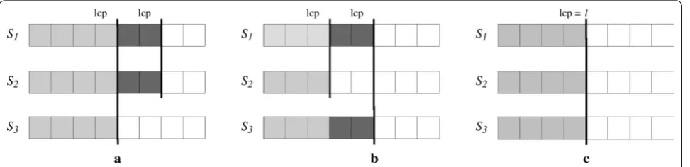
lcp values can be used to speed up suffix comparisons [9, 43] and to avoid external memory accesses in heap inser-tions. The following lemma formalizes the idea. The proof is simple, based on the cases illustrated in Fig. 1, and will be omitted.
Lemma 1 Let S1,S2andS3be strings, such that S1<S2 and S1<S3. Iflcp(S1,S2) >lcp(S1,S3)thenS2<S3(case 1). Iflcp(S1,S2) <lcp(S1,S3)thenS2>S3(case 2). Oth-erwise, iflcp(S1,S2)=lcp(S1,S3)=ℓthenlcp(S2,S3)≥ℓ
(case 3).
Let X, Y and Z be nodes in the binary heap storing Ea[i],Eb[j] and Ec[k], respectively. Let X, Y and Z be also
the suffixes stored by such heap nodes. Suppose that
node X is the parent of Y and Z. Because X<Y and
X<Z it follows that Ta[SAa[i],na]<Tb[SAb[j],nb] and
Ta[SAa[i],na]<Tc[SAc[k],nc]. Assume that the heap
also stores lcp values between a node and its children and
between a node and its sibling.
As X is removed from the heap, Ea[i] is moved to the output buffer and X is replaced by another node W stor-ing Ea[i+1]. The order of W with respect to its children Y and Z can be determined without character compari-sons when case 1 or case 2 of Lemma 1 applies, and if case 3 applies then the character comparison can be started from symbol ℓ=lcp(X,W), recalling that lcp(X,W) is stored in Ea[i+1]. In the same way the order between Y and Z can be determined using Lemma 1. Algorithm 3 illustrates this procedure to compare the nodes W, Y and Z in the heap.
lcp values between nodes in the heap are updated as
nodes are compared and swapped. Suppose that node W is swapped with Y (meaning Y <W and Y <Z). The
lcp of W with respect to its new children are also
deter-mined using Lemma 1, taking the minimum lcp between
two suffixes (in cases 1 and 2) or through direct charac-ter comparisons (case 3). Hence, by using lcp values many
direct comparisons of strings that are in external mem-ory are avoided.
Table 4 An example of a part of ESA1 illustrating the prefix assembly strategy
Symbols in bold highlight the substring of suffix T1[SA[6],n1] stored in PREFIX1
For instance, consider merging ESA1 and ESA2
in Table 1. First, comparing the elements ESA1[4]
and ESA2[3] we conclude that suff
2(3)=AGA$ is less than suff1(4)=ATAGA$. The next
com-parison involves ESA1[4] and ESA2[4]. As already
stated, without comparing any symbols we see that lcp(suff2(3),suff2(4)) >lcp(suff2(3),suff1(4)) and that
suff2(4)=AGAGA$ is less than suff1(4)=ATAGA$.
Suffix induction
The induced sorting principle corresponds to deduce the order of unsorted suffixes from already sorted suffixes. This strategy is used by many suffix array construction algorithms [49]. We apply an induced sorting approach that relies on the following lemma. Let a suffix starting with a symbol α be denoted α-suffix and let suffT be the
set of all suffixes of strings in T.
Lemma 2 IfTi[j,ni]is the smallest suffix insuffT then Ti[j−1,ni] =α·Ti[j,ni] is the smallest α-suffix in suffT \ {Ti[j,ni]}.
Proof Suppose that there is a α-suffixTℓ[k,nℓ] in suffT
that precedes Ti[j−1,ni]. Then Tℓ[k+1,nℓ] must be
smaller than Ti[j,ni], a contradiction.
Lemma 2 can be used for sorting the suffixes of a string T of length n as follows. Let an α-bucket be a block of a
partition of SA that contains only α-suffixes. suff
T is
ini-tialized with every suffix of T and an empty bucket for each symbol in is created. While suffT is not empty,
the smallest suffix T[j,n] =α·T[j+1,n] in suffT is
moved to the leftmost available position in the α-bucket
and, if α < β then T[j−1,n] =β·T[j,n] is added to the leftmost available position in the β-bucket (it is induced).
The induced suffix T[j−1,n] cannot be removed from suffT yet because it may induce T[j−2,ni] as well. When
a suffix that is already in a bucket is also the smallest in
suffT, the suffix itself and those that succeed it in the
bucket are used to induce another suffix and are removed from suffT at once. Note that if α > β then the suffix T[j−1,ni] was already sorted and if α=β then reading
induced suffixes from the β-bucket can cause the
induc-tion of already induced suffixes. So no inducinduc-tion is done when α≥β.
This approach is not efficient to sort the suffixes of a single string T, since it is often necessary to find a small-est suffix. But in merging previously sorted suffixes the smallest one can be determined efficiently using the heap. Suppose that Ei[k] is at the root of the heap. Then
Ti[j,ni] is the smallest suffix in suffT and Ti[j−1,ni]
can be induced if Ti[j]<Ti[j−1]. This later test may be
performed using BWTi and, as a consequence, to deter-mine whether Ti[j−1,ni] can be induced or not.
Induced suffixes are added to the induced buffer I, par-titioned into buckets Iα, one for each α∈�. When an α -suffix from string Ti is induced, the value i is inserted
into the first available position of Iα, which is written to an external memory file Fα as it gets full. When the smallest α-suffix is at the root of the heap, Fα is read sequentially to retrieve string indexes. Each string index i indicates that the smallest suffix in Ei may be written to the output directly, since such suffix has been induced, bypassing operations in the heap and saving many com-parisons. When every index in Fα has been processed the heap must be reconstructed. Algorithm 4 illustrates Phase 2 (see Algorithm 1) augmented for suffix induc-tion. Whenever the first suffix starting with α=Ta[b] is returned from the heap, eGSA induces the output buffer
the suffixes in Fα.
lcp values for induced suffixes must also be induced,
since induced suffixes are not compared in the heap. Suppose that Ta[i,na] induces an α-suffix and
sup-pose that Tb[j,nb] induces the next α-suffix. Then LCP(Ta[i−1,na],Tb[j−1,nb])=LCP(Ta[i,na],Tb[j,nb])+1.
But since Ta[i,na] and Tb[j,nb] may not be
consecu-tive in GSA, LCP(Ta[i,na],Tb[j,nb]) may not be obtained directly. Such value may be obtained from the range minimum query on the LCP, defined as rmq(x,y)=minx≤k≤y{LCP[k]}. It is easy to see that as Ta[i,na] and Tb[j,nb] are already sorted
and LCP(Ta[j,na],Tb[j,nb])=rmq(pos(Ta[j,na] +1), pos(Tb[j,nb])) the rmq value may be computed as LCP values are moved to the output buffer.
Therefore, when a suffix Ti[j,ni] is induced in the
induced suffixes may also induce further suffixes, the cor-responding LCP must be stored in the induced buffer Iα and in the respective file as well. As induced suffixes are recovered from external memory, LCP values are recov-ered to update the rmq computation.
For instance, suppose that T1[6,n1] =A$ is the small-est suffix in the heap during the merge of ESA1 and ESA2 in Table 1. Because ESA1[2].BWT=G>A, T1[6−1=5,n1] =GA$ is induced as the smallest G
-suf-fix in suffT. Then the pair (1, 0) is written to the buffer IG
to indicate that a suffix from string 1 was induced with
lcp=0. The lcp value in GESA between T1[5,n1] and the
next induced G-suffix (T2[5,n2]) is computed by the mini-mum lcp value from the suffixes passing through the heap
until T2[5,n2] is induced. This happens when T2[6,n2] is the smallest element in the heap and T2[5,n2] is induced together with the lcp(T1[6,n1],T2[6,n2])+1=2,
obtained by the current minimum lcp value. When T1[5,n1] is the smallest suffix in the heap, FG is read sequentially and the induced G-suffixes are recovered together with their lcp values.
Using prefix assembly together with induction requires additional care. Since induced suffixes are not compared in the heap, they do not participate in the prefix assem-bly. Thus during the evaluation of PREFIX in Phase 1,
hj must be equal to 0 for every last α-suffix that will be
induced, then the prefix of the first non-induced α
-suf-fix will start at its initial position. To this end, we set 0 as the LCP[pos(Ti[j,ni])] of every suffix Ti[j,ni] that will be induced, i.e. when Ti[j]>Ti[j+1]. Recall that all such lcp values will be also induced.
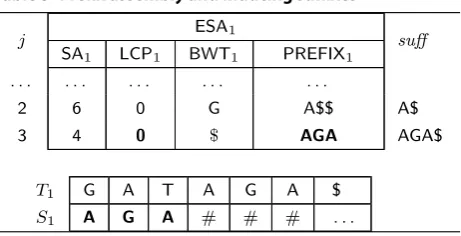
For instance, Table 5 illustrates the construction of
ESA1 in the first phase of eGSA, for j=2. When j=2, SA[j=2] =6 and T1[6]>T1[6+1], then the suffix T1[6,n1] will be induced and LCP1[2+1=3] receives
0. Next, j=3,SA[j=3] =4 and T1[4]<T1[4+1], the
suffix T1[4,n1] will not be induced. It means that, in the
second phase, T1[6,n1] will be induced and bypassed in the heap, thus the prefix assembling of suffix T1[4,n1]
must start from scratch in S1. From this point, prefix assembly continues normally.
Theoretical costs
Phase 1 of eGSA is dominated by the algorithms used to
construct SA and LCP. The other columns of the general-ized suffix array are evaluated when the output is written to disk, using constant time and memory per item. The construction of SA and LCP may be done in linear time and space [29, 46]. Thus, for m input strings with total length N and Tℓ the longest string, Phase 1 is O(m|Tℓ|)
time plus O(N) I/O operations using O(|Tℓ|) memory.
In Phase 2, the number of node swaps in the heap is bounded by Nlogm. Each node swap requires
compar-ing a number of characters that is at most the maximum value of lcp for T (maxlcp). The time cost of this phase
is then O((Nlogm)maxlcp). I/O operations in Phase 2
include loading portions of suffix arrays and of strings from disk, and writing output buffers to disk. Suffix arrays are loaded in blocks to the enhanced-array buffers. In the worst case each comparison in the heap will trig-ger a character comparison, and the string buffers will be loaded when exhausted. Provided that the string buffer is at least as large as maxlcp, each suffix will cause at most
one I/O operation and the worst case for the number of string buffer load operations is O(N). The number of I/O operations on enhanced-array and output buffers is lim-ited by N divided by the respective buffer sizes. Then the number of I/O operations in Phase 2 is bounded by O(N). The memory usage in Phase 2 is bounded by the sum of buffer sizes, which can be tailored as necessary.
Such bounds for I/O operations are prohibitive, but it is much lower in practice due to the optimizing strategies, as shown in the next sections. An easy to devise limita-tion of eGSA is the case of datasets whose strings are large
and highly repetitive, for instance, a dataset composed by human genomes of different individuals. For these data-sets the practical performance will approach the theoretical bound. Another limitation is when maxlcp is larger than the
string buffer size, when the number of I/O operations is as bad as O(Nlogm(|Tℓ|/s)), where s is the string buffer size.
Performance evaluation
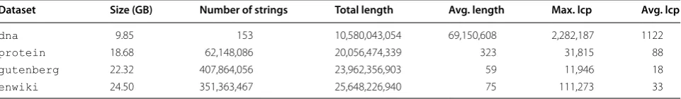
We used four real datasets of different domains, including DNA and protein sequences, and natural language texts as described in Table 6. The table includes the total size of each dataset in GB, the number of strings, the average string length, and the average and maximum lcp values, which
provide an approximation of suffix sorting difficulty [16]. The experiments were conducted on Debian GNU/ Linux 6.0.3/64 bits operating system using an Intel(R) Xeon(R) CPU E3-1230 V2 @ 3.30 GHz processor 8 MB cache, with 32 GB of internal memory and a 2.0 TB
Table 5 Prefix assembly and inducing suffixes
SATA hard disk with 7200 RPM and 64 MB cache (Sea-gate Desktop HDD ST2000DM001). Our algorithm was implemented in ANSI/C and compiled by GNU GCC version 4.6.3, with optimizing option -O3. The source code is freely available at https://github.com/felipelouza/ egsa/.
In Phase 1 we partitioned the collection of strings T
into k groups, such that when the strings in each group are concatenated the resulting string Tcat may be given to
internal memory SA and LCP construction algorithms. After concatenating the strings in a group a new termina-tor symbol # that is smaller than $ is added to the end of Tcat. For the first phase we used gSACA-K [36] combined
with -algorithm [29]. gSACA-K guarantees that the order of equal suffixes from different strings in a group will be defined by the rank of their strings in T. Given the SA of Tcat, we compute GSA for the string group using
an additional integer array DA of size |Tcat| that stores in DA[i] the string to which suffix Tcat[i,|Tcat|] belongs
in T.DA can be computed easily by scanning Tcat. Then,
each value SA[i] is mapped to GSA[i].str and GSA[i].suff,
and the GSA for the string group is written to
exter-nal memory. ESA[i], that will be used in Phase 2, will
be composed by �GSA[i],LCP[i],BWT[i],PREFIX[i]�. The -algorithm was adapted to stop the comparison in
Tcat when it reaches $ symbols, thus correctly evaluating
the LCP between suffixes in the same group. Together, these algorithms use 13× |Tcat| bytes. In this
experi-ments, when Tcat is composed by only one string Tℓ and 13× |Tcat| is larger than the available internal memory,
the algorithm truncates Tℓ, such that 13× |Tcat| fits in
memory. The sizes reported in Table 6 refer to the data-sets after truncations, that happened only with dna.
In Phase 2 we used p=10 for the prefix array size, which provided a good tradeoff between time and disk usage space, as shown in "eGSA internals" section. Each buffer Si were set to use 20 KB of internal memory,
whereas all buffers B, Bufferout and I were set to use 1 GB,
64 MB and 16 MB, respectively, in total. We remark that
eGSA uses 1 byte to store each character in memory. The
output produced by eGSA was validated using a trivial
checking algorithm.
In "Relative performance" section we investigate the behavior of eGSA with respect to eSAIS [10] and
SAscan [27]. In "eGSA internals" section we evaluate eGSA in detail, showing the influence of each phase and
of the improving strategies used in Phase 2 on the total running time. In "Limitations" section we investigate limitations of our algorithm related to the effect of disk cache managed by the operating system when the inter-nal memory (RAM) size is restricted at boot time.
Relative performance
To assess the performance of eGSA we compared it to
eSAIS [11], which is the fastest algorithm to date to compute both suffix and LCP arrays in external memory. We also compared eGSA to SAscan [28], which
com-putes only the suffix array with small peak disk usage. We configured the algorithms to use the same disk for input and output. We are aware of the existence of the algo-rithms by Bauer et al. [5, 6] and by Cox et al. [13] that aim at indexing collections of small strings in external memory. However, we did not consider comparing them with eGSA because they were designed to solve a
differ-ent problem, namely building the BWT and the LCP array with small memory footprint. Moreover, a comparison in the article [13] have shown that eGSA is faster and uses
more space in external memory.
Although eSAIS and SAscan are aimed at
index-ing only one strindex-ing, we can concatenate all strindex-ings and use eSAIS or SAscan to construct the generalized
suf-fix arrays. All strings in T were concatenated and a final
terminator # was added, such that #<$. This concatena-tion strategy will not guarantee that equal suffixes will be sorted by string rank and the values in LCP may be larger than the actual lcp of consecutive suffixes in GESA, Table 6 Datasets used in the experiments
dna:a collection of large DNA chromosomes from organisms (Homo sapiens, Oryzias latipes, Danio rerio, Bos taurus, Mus musculus and Gallus gallus) of Ensembl dataset (ftp://ftp.ensembl.org/pub/release-84/fasta/). We removed any occurrences of the character N (unknown) from the strings
protein: the collection of protein sequences from Uniprot/TrEMBL, release 2016_5 (http://www.ebi.ac.uk/uniprot/download-center/)
gutenberg: a collection of documents from Gutenberg Project, release 2012_09 (http://algo2.iti.kit.edu/bingmann/esais-corpus/). We processed each line of the input as a single string
enwiki: a collection of pages from a snapshot of the English language edition of Wikipedia release 2016_05 (https://dumps.wikimedia.org/enwiki/20160501/). We processed each line of the input as a single string
Dataset Size (GB) Number of strings Total length Avg. length Max. lcp Avg. lcp
dna 9.85 153 10,580,043,054 69,150,608 2,282,187 1122
protein 18.68 62,148,086 20,056,474,339 323 31,815 88
gutenberg 22.32 407,864,056 23,962,356,903 59 11,946 18
but will not impose the growth of the alphabet size and still allows eSAIS and SAscan to use 1 byte per input
character.
We remark that the results presented in this section depends on the RAM size available in the experiments, that is, 32 GB. As we show in "Limitations" section, the performance and efficiency of eGSA degrades as the
total RAM size is reduced.
Running time and efficiency
Figure 2 shows the running time in microseconds per input byte and the efficiency of eGSA, eSAIS and
SAscan. Efficiency is the proportion of time for which
the CPU is busy, not waiting for I/O. Except for dna, eSAIS was interrupted for datasets with more than 12 GB due to the large amount of time to process these instances. For example, eSAIS took 9 days to run on
enwiki with 12 GB. The experiments took about 70 days of computing to finish.
The amount of internal memory used by the algo-rithms is an input parameter. We configured them to use 2 GB. Although the comparison is not totally fair because eSAIS and SAscan were not designed for
mul-tiple strings, eGSA have outperformed eSAIS and pre-sented a competitive performance compared to SAscan,
which computes only the SA. Moreover, eGSA can also
construct the generalized BWT of the collection T with no additional cost except by the output time.
The long running times of eSAIS prevented the analy-sis of its efficiency trend. In the extreme case, enwiki
with 12 GB, the running time of eSAIS is almost 35 times larger than the time spent by eGSA. The running times
of eGSA and SAscan are very close, with larger
differ-ences only for the dna dataset. SAscan presents the best
efficiency, which is mostly unaffected by the size of the dataset. The efficiency of eGSA is comparable to SAscan
for small datasets and better than the efficiency of eSAIS. The efficiency of eGSA drops with the size of the
data-set. For larger datasets it becomes apparent that the effi-ciency of eGSA is strongly affected by the effect of the
disk cache managed by the operating system, since the size of the available internal memory decreases as the dataset increases (we evaluate this issue in "Limitations" section).
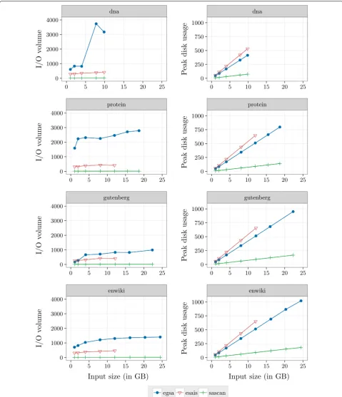
I/O volume and peak disk usage
The I/O volume (in bytes per input byte) and the peak disk usage (in GB) of each algorithm are reported in Fig. 3. eGSA makes a larger volume of I/O transfer. In
the extreme case, protein with 12 GB, eGSA transfer
more than 6 times data than eSAIS and eGSA transfers
150 times more data than SAscan.eGSA uses 39n bytes
(8n bytes for GSA, 4n bytes for LCP, and 27n bytes for
auxiliary structures) plus by the size of the temporary files used to store induced suffixes. As can be seen in Fig. 5, the average number of induced suffixes is about 43%, and is almost constant for all dataset sizes. eSAIS uses 54n bytes to compute SA and LCP arrays, whereas SAscan uses 7.5n bytes to compute SA. Overall, the peak
disk usage is much smaller for SAscan.
Although eSAIS and SAscan do not take care of the
peculiarities of a generalized suffix array, eGSA still
shows faster or comparable running times. Therefore,
eGSA is a good alternative for the construction of the
generalized enhanced suffix array in external memory.
eGSA internals
We have evaluated the behavior of eGSA in terms of the
performance of each phase and the effect of each heap strategy used in Phase 2.
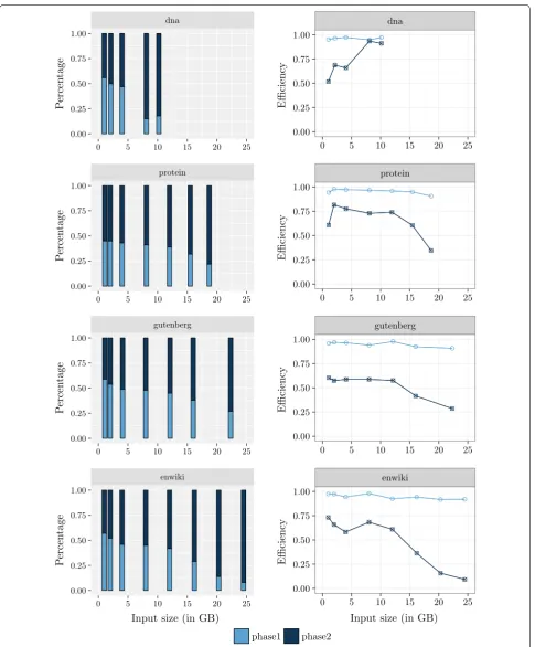
Figure 4 shows the percentage of time spent by each phase of eGSA and its efficiency. We can see that the
percentage of the time spent by Phase 2 increases as the dataset increases and dominates the time of eGSA. We
can see that the efficiency of Phase 1 is almost constant and the efficiency of Phase 2 is better for small alphabets (dna).
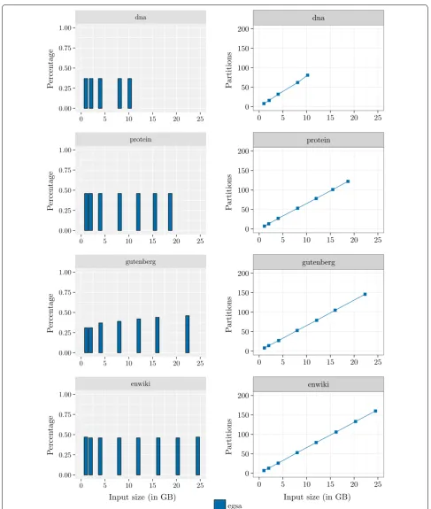
Figure 5 shows the percentage of induced suffixes and the number of partitions created by eGSA in the
pre-processing step. In the average, 42% of the suffixes were
induced. This indicates that the algorithm is avoiding many string comparisons. The number of partitions grows linearly with the dataset size, and the figure shows Phase 1 using less than 2 GB.
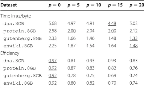
Prefix array size
We have analyzed the effect of the value of the parameter p on the running time. We used the first 8 GB of each dataset for these experiments. Recall that p is the num-ber of symbols in each position of PREFIX arrays and has
a major impact on external memory usage and access. As the value of p grows the external memory access decreases but the peak disk space usage increases. We evaluated some values for p with fixed memory usage, that is, increasing p implied an reduction of the number of elements in the partition buffers Bi, guaranteeing that
all versions use the same amount of internal memory. Table 7 shows the effect of p on the total running time and the efficiency of eGSA, for p varying between 0 and
25. The value p=10 resulted in a good tradeoff between the peak disk space used by the algorithm and the run-ning time.
Effect of optimizations
dna
0.0 2.5 5.0 7.5 10.0 12.5
0 5 10 15 20 25
Running
time
dna
0.00 0.25 0.50 0.75 1.00
0 5 10 15 20 25
Efficiency
protein
0.0 2.5 5.0 7.5 10.0
0 5 10 15 20 25
Running
time
protein
0.00 0.25 0.50 0.75 1.00
0 5 10 15 20 25
Efficiency
gutenberg
0.0 2.5 5.0 7.5 10.0
0 5 10 15 20 25
Running
tim
e
gutenberg
0.00 0.25 0.50 0.75 1.00
0 5 10 15 20 25
Efficiency
enwiki
0 20 40 60
0 5 10 15 20 25
Input size (in GB)
Running
tim
e
enwiki
0.00 0.25 0.50 0.75 1.00
0 5 10 15 20 25
Input size (in GB)
Efficiency
egsa esais sascan
Fig. 2 Running time. Running time in microseconds per input byte and the efficiency of eGSA,eSAIS and SAscan. Efficiency is the proportion of time for which the CPU is busy, not waiting for I/O. The running time of eGSA is consistently smaller than that of eSAIS and comparable to
assembly, (b) LCP comparison and (c) suffix induction,
every possible combination of them was tested. Again, we used the first 8 GB of each dataset. The running time and the efficiency for each dataset is shown in Table 8. dna
0 1000 2000 3000 4000
0 5 10 15 20 25
I/O
volume
dna
0 250 500 750 1000
0 5 10 15 20 25
P
eak
disk
usage
protein
0 1000 2000 3000 4000
0 5 10 15 20 25
I/
Ov
olume
protein
0 250 500 750 1000
0 5 10 15 20 25
Pe
ak
disk
usage
gutenberg
0 1000 2000 3000 4000
0 5 10 15 20 25
I/
Ov
olume
gutenberg
0 250 500 750 1000
0 5 10 15 20 25
Pe
ak
disk
usage
enwiki
0 1000 2000 3000 4000
0 5 10 15 20 25
Input size (in GB)
I/
Ov
olume
enwiki
0 250 500 750 1000
0 5 10 15 20 25
Input size (in GB)
Pe
ak
disk
usage
egsa esais sascan
dna
0.00 0.25 0.50 0.75 1.00
0 5 10 15 20 25
P
ercen
tage
dna
0.00 0.25 0.50 0.75 1.00
0 5 10 15 20 25
Efficiency
protein
0.00 0.25 0.50 0.75 1.00
0 5 10 15 20 25
P
ercen
tage
protein
0.00 0.25 0.50 0.75 1.00
0 5 10 15 20 25
Efficiency
gutenberg
0.00 0.25 0.50 0.75 1.00
0 5 10 15 20 25
Pe
rcen
tage
gutenberg
0.00 0.25 0.50 0.75 1.00
0 5 10 15 20 25
Efficiency
enwiki
0.00 0.25 0.50 0.75 1.00
0 5 10 15 20 25
Input size (in GB)
Pe
rcen
tage
enwiki
0.00 0.25 0.50 0.75 1.00
0 5 10 15 20 25
Input size (in GB)
Efficiency
phase1 phase2
dna
0.00 0.25 0.50 0.75 1.00
0 5 10 15 20 25
P
ercen
tage
dna
0 50 100 150 200
0 5 10 15 20 25
P
artitions
protein
0.00 0.25 0.50 0.75 1.00
0 5 10 15 20 25
P
ercen
tage
protein
0 50 100 150 200
0 5 10 15 20 25
P
artitions
gutenberg
0.00 0.25 0.50 0.75 1.00
0 5 10 15 20 25
P
ercen
tag
e
gutenberg
0 50 100 150 200
0 5 10 15 20 25
P
artitions
enwiki
0.00 0.25 0.50 0.75 1.00
0 5 10 15 20 25
Input size (in GB)
P
ercen
tag
e
enwiki
0 50 100 150 200
0 5 10 15 20 25
Input size (in GB)
P
artitions
egsa
We can see that the complete version of eGSA
(col-umn {a,b,c}) was the best in the majority of the cases.
The dataset gutenberg.8GB was faster using {a,b}
with a difference of about 10%. Comparing with the ∅ version, optimization strategies reduced the time by a factor of 1.9−2.22. Note that all strategies individually improved performance with respect to the ∅ version. Thus, we may conclude that the use of heap strategies heavily improves the performance of eGSA. As a final
remark, we note that, except for dna.8GB, the ∅ version reduced the time by a factor of up to 6.10 compared with eSAIS (Fig. 2).
Limitations
We have investigated the effect of the disk caching in the performance of eGSA,eSAIS and SAscan. We restricted
both the internal memory available to our algorithm (2 GB) as well as the total system memory at boot time (8−24 GB).
Table 9 shows the running time and the efficiency of each algorithm set to use 2 GB of internal memory to process the first 8 GB of the dataset dna in a machine whose total RAM was restricted to 24, 16, 12, 10 and 8 GB at boot time. The values in the last column (32 GB) are the same presented in "Relative performance" and "eGSA internals" sections. We also tested the datasets
protein.8GB, gutenberg.8GB and enwiki.8GB
and we obtained very close results, which were omitted. The running time and efficiency of each algorithm degrade as the total RAM size reduces. This happens as an effect of the reduction of free memory available for disk caching managed by the operating system, which reduces the number of disk accesses. Comparing to the original setting (32 GB), the running time of eGSA was
about 25 times larger with the RAM size restricted to 8 GB, whereas for eSAIS and SAscan their running times
were about 1.3 larger.
For eGSA, disk caching reduces disk accesses to the
input strings as suffixes are moved along the heap, which displays a “random” pattern. This is where the worst case complexity stated in "Theoretical costs" section shows its claws. On the other hand, eGSA takes advantage of the
disk cache system, which might be a favorable aspect in practical setups. Recall that the total size of the output data structure is 12 times the dataset size, which is 96 GB for the dataset dna.8GB.
The experiments show that eGSA depends on the
availability of a large amount of free RAM to be effi-cient, which can be seen as a feature of a semi-external algorithm [8]. However, eGSA works purely in
exter-nal memory. We believe that the optimizing strategies applied on the heap are interesting per se, and, as the disk access pattern is not actually random, may be there is still room for improving the overall strategy based on a heap, what could improve the performance of eGSA with less
support of disk caching.
Table 7 Time spent by eGSA according to the prefix array
size
The experiment with p=10 is the same presented in Figs. 2, 3, 4 and 5 and
p=0 means that the prefix assembly strategy was not used by the algorithm
Dataset p=0 p=5 p=10 p=15 p=20
Time in µs/byte
dna.8GB 5.68 4.97 4.91 4.48 5.03
protein.8GB 2.58 2.00 2.04 2.00 2.12
gutenberg.8GB 2.33 1.66 1.46 1.48 1.33
enwiki.8GB 2.25 1.87 1.54 1.64 1.48
Efficiency
dna.8GB 0.97 0.81 0.93 0.93 0.83
protein.8GB 0.92 0.87 0.83 0.82 0.76
gutenberg.8GB 0.92 0.78 0.75 0.69 0.74
enwiki.8GB 0.92 0.80 0.82 0.70 0.74
Table 8 Effect of each heap strategies on time
All possible combinations of (a) prefix assembly, (b) LCP comparison and (c) suffix induction are plotted for the datasets. ∅ is the case when none of them is used, and {b,c} and {a,b,c} are the same presented in columns p=0 and p=10 of Table 7
Dataset ∅ {a} {b} {c} {a, b} {a, c} {b, c} {a, b, c}
Time in µs/byte
dna.8GB 10.08 8.13 8.52 6.79 6.43 5.60 5.68 4.91
protein.8GB 3.88 2.74 3.49 2.76 2.26 2.15 2.58 2.04
gutenberg.8GB 3.18 1.48 2.96 2.47 1.35 1.55 2.33 1.46
enwiki.8GB 3.28 1.87 3.04 2.42 1.73 1.82 2.25 1.54
Efficiency
dna.8GB 0.98 0.97 0.98 0.98 0.95 0.95 0.97 0.93
protein.8GB 0.95 0.88 0.96 0.94 0.89 0.87 0.92 0.83
gutenberg.8GB 0.95 0.83 0.95 0.93 0.77 0.77 0.92 0.75
Conclusions
In this article we proposed eGSA, which is the first
exter-nal memory algorithm to construct generalized suffix arrays enhanced with the longest common prefix array (LCP) and the Burrows–Wheeler transform (BWT) for a collection of strings. The proposed algorithm was vali-dated through performance tests using real datasets from different domains, in various combinations. Compared to eSAIS and SAscan,eGSA showed a competitive
perfor-mance. Moreover, our algorithm can also constructs the generalized BWT of a collection of strings with no addi-tional cost except by the output time.
Another advantage of eGSA is that it may be employed
to build generalized enhanced suffix arrays from arrays that have already been computed individually for strings in a dataset. Moreover, eGSA may be used to construct
the core data structures used by LOF-SA [50] and ROSA search algorithms [21], or to build generalized suffix trees in external memory [4]. Furthermore, it may be applied to solve the longest common substring problem [1, 3] and to construct the Longest Previous Factor array, which is used in text compression and for detecting motifs and repeats [15].
Authors’ contributions
FAL, GPT and CDAC devised the algorithm. FAL and GPT implemented the algorithm and performed experiments with major contributions by SH. All authors read and approved the final manuscript.
Author details
1 Department of Computing and Mathematics, University of São Paulo, Av. Bandeirantes, 3900, Ribeirão Preto 14040-901, Brazil. 2 Institute of Computing, University of Campinas, Av. Albert Einstein, 1251, Campinas 13083-852, Brazil. 3 Computational Biology, Leibniz Institute on Aging - Fritz Lipman Institute and Friedrich Schiller University Jena, Beutenbergstrasse 11, Jena 07745, Germany. 4 Institute of Mathematics and Computer Science, University of São Paulo, Av. Trabalhador São-carlense, 400, São Carlos 13560-970, Brazil.
Acknowledgements
We thank the anonymous reviewers for comments that improved the pres-entation of the manuscript. The authorsthank Pedro Hokama and Prof. Nalvo Almeida for granting access to the machines used for the experiments.
Competing interests
The authors declare that they have no competing interests.
Availability of data and materials Not applicable.
Consent for publication Not applicable.
Ethics approval and consent to participate Not applicable.
Funding
FAL was supported by the Grants #2011/15423-9 and #2017/09105-0 from the São Paulo Research Foundation (FAPESP). GPT acknowledges the financial sup-port of CNPq and FAPESP. SH acknowledges the financial supsup-port of Leipzig Research Center for Civilization Diseases (LIFE), Leipzig University. LIFE is funded by the European Union, by the European Regional Development Fund (ERDF), the European Social Fund (ESF) and by the Free State of Saxony within the excellence initiative. CDAC has been supported by Brazilian agencies CAPES, CNPq, FAPESP [Grant Number 2011/23904-7] and FINEP.
Publisher’s Note
Springer Nature remains neutral with regard to jurisdictional claims in pub-lished maps and institutional affiliations.
Received: 13 July 2017 Accepted: 22 November 2017
References
1. Arnold M, Ohlebusch E. Linear time algorithms for generalizations of the longest common substring problem. Algorithmica. 2011;60(4):806–18. 2. Abouelhoda MI, Kurtz S, Ohlebusch E. Replacing suffix trees with
enhanced suffix arrays. J Discret Algorithms. 2004;2(1):53–86.
3. Babenko MA, Starikovskaya T. Computing longest common substrings via suffix arrays. In: Proceedings of computer science in Russia symposium. 2008. p. 64–75.
4. Barsky M, Stege U, Thomo A. Suffix trees for inputs larger than main memory. Inform Syst J. 2011;36(3):644–54.
5. Bauer MJ, Cox AJ, Rosone G. Lightweight algorithms for construct-ing and invertconstruct-ing the BWT of strconstruct-ing collections. Theor Comput Sci. 2013;483:134–48.
6. Bauer MJ, Cox AJ, Rosone G, Sciortino M. Lightweight LCP construction for next-generation sequencing datasets. In: Proceedings of WABI. Berlin: Springer; 2012. p. 326–37.
7. Beller T, Gog S, Ohlebusch E, Schnattinger T. Computing the longest common prefix array based on the Burrows–Wheeler transform. J Discret Algorithms. 2013;18:22–31.
8. Beller T, Zwerger M, Gog S, Ohlebusch E. Space-efficient construction of the Burrows–Wheeler transform. Proc SPIRE. 2013;8214:5–16.
9. Bingmann T, Eberle A, Sanders P. Engineering parallel string sorting. Algorithmica. 2015;77:1–52.
Table 9 Time spent by eGSA,eSAIS and SAscan to process dna.8GB according to the total RAM size
Algorithm 8 GB 10 GB 12 GB 16 GB 24 GB 32 GB
Time in µs/byte
eGSA 112.89 34.36 10.14 5.65 4.63 4.60
eSAIS 12.17 11.16 11.55 10.62 11.39 9.36
SAscan 2.10 1.71 1.83 1.70 1.59 1.65
Efficiency
eGSA 0.05 0.33 0.43 0.76 0.92 0.92
eSAIS 0.66 0.65 0.63 0.68 0.64 0.74
• We accept pre-submission inquiries
• Our selector tool helps you to find the most relevant journal • We provide round the clock customer support
• Convenient online submission • Thorough peer review
• Inclusion in PubMed and all major indexing services • Maximum visibility for your research
Submit your manuscript at www.biomedcentral.com/submit
Submit your next manuscript to BioMed Central
and we will help you at every step:
10. Bingmann T, Fischer J, Osipov V. Inducing suffix and LCP arrays in external memory. ACM J Exp Algorithmics. 2016;21(2):2.3:1–27.
11. Bingmann T. eSAIS. https://tbingmann.de/2012/esais. Accessed Jun 2017. 12. Burrows M, Wheeler DJ. A block-sorting lossless data compression
algorithm. Digital SRC Research Report. 1994. http://citeseerx.ist.psu.edu/ viewdoc/summary?doi=10.1.1.121.6177
13. Cox AJ, Garofalo F, Rosone G, Sciortino M. Lightweight LCP construction for very large collections of strings. J Discret Algorithms. 2016;37:17–33. 14. Crauser A, Ferragina P. A theoretical and experimental study on
the construction of suffix arrays in external memory. Algorithmica. 2002;32(1):1–35.
15. Crochemore M, Grossi R, Kärkkäinen J, Landau GM. A constant-space comparison-based algorithm for computing the Burrows–Wheeler trans-form. In: Proceedings of CPM. Berlin: Springer; 2013. p. 74–82.
16. Dementiev R, Kärkkäinen J, Mehnert J, Sanders P. Better external memory suffix array construction. ACM J Exp Algorithmics. 2008;12:3.4:1–24. 17. Dhaliwal J, Puglisi SJ, Turpin A. Trends in suffix sorting: a survey of low
memory algorithms. In: Proceedings of ACSC. Canberra: ACSC; 2012. p. 91–8.
18. Ferragina P, Gagie T, Manzini G. Lightweight data indexing and compres-sion in external memory. Algorithmica. 2012;63(3):707–30.
19. Fischer J. Inducing the LCP-array. In: Proceedings of WADS. Ansonia: WADS; 2011. p. 374–85.
20. Flick P, Aluru S. Parallel distributed memory construction of suffix and longest common prefix arrays. In: Proceedings of SC. Carolina: SC; 2015. p. 16:1–10.
21. Gog S, Moffat A, Culpepper JS, Turpin A, Wirth A. Large-scale pattern search using reduced-space on-disk suffix arrays. IEEE Trans Knowl Data Eng. 2014;26(8):1918–31.
22. Gog S, Ohlebusch E. Fast and lightweight LCP-array construction algo-rithms. In: Proceedings of ALENEX. Barcelona: ALENEX; 2011. p. 25–34. 23. Gonnet GH, Baeza-Yates RA, Snider T. New indices for text: pat trees and
pat arrays. In: information retrieval. Upper Saddle River: Prentice-Hall, Inc.; 1992. p. 66–82.
24. Gusfield D. Algorithms on strings, trees, and sequences: computer sci-ence and computational biology. New York: Cambridge University Press; 1997.
25. Kärkkäinen J, Kempa D. Engineering a lightweight external memory suffix array construction algorithm. In: Proceedings of ICABD. 2014. p. 53–60. 26. Kärkkäinen J, Kempa D. LCP array construction in external memory. ACM
J Exp Algorithmics. 2016;21:1–22.
27. Kärkkäinen J, Kempa D, Puglisi SJ. Parallel external memory suffix sorting. In: Proceedings of CPM. 2015. p. 329–42.
28. Kärkkäinen J, Kempa D. SAscan. https://www.cs.helsinki.fi/group/pads/ SAscan.html. Accessed Jun 2017.
29. Kärkkäinen, J., Manzini, G., Puglisi, S.J.: Permuted longest-common-prefix array. In: Proceedings of CPM. 2009. p. 181–92.
30. Kärkkäinen J, Sanders P, Burkhardt S. Linear work suffix array construction. ACM J. 2006;53(6):918–36.
31. Kasai T, Lee G, Arimura H, Arikawa S, Park K. Linear-time longest-common-prefix computation in suffix arrays and its applications. In: Proceedings of CPM. 2001. p. 181–92.
32. Knuth DE. The art of computer programming. Sorting and searching, vol. 3. 2nd ed. Redwood City: Addison Wesley Longman Publishing Co.; 1998. 33. Ko P, Aluru S. Space efficient linear time construction of suffix arrays. J
Discret Algorithms. 2005;3(2–4):143–56.
34. Liu WJ, Nong G, Chan WH, Wu Y. Induced sorting suffixes in external memory with better design and less space. In: Proceedings of SPIRE. Bengaluru: SPIRE; 2015. p. 83–94.
35. Louza FA, Gog S, Telles GP. Optimal suffix sorting and LCP array construc-tion for constant alphabets. Inf Process Lett. 2017;118:30–4.
36. Louza FA, Gog S, Telles GP. Inducing enhanced suffix arrays for string col-lections. Theor Comput Sci. 2017;678:22–39.
37. Louza FA, Gagie G, Telles GP. Burrows–Wheeler transform and LCP array construction in constant space. J Discret Algorithms. 2017;42:12–22. 38. Louza FA, Telles GP, Ciferri CDA. External memory generalized suffix and
LCP arrays construction. In: Proceedings of CPM. 2013. p. 201–10. 39. Mäkinen V, Belazzougui D, Cunial F. Genome-scale algorithm design. New
York: Cambridge University Press; 2015.
40. Manber U, Myers EW. Suffix arrays: a new method for on-line string searches. SIAM J Comput. 1993;22(5):935–48.
41. Manzini G. Two space saving tricks for linear time LCP array computation. In: Proceedings of SWAT. 2004. p. 372–83.
42. Munro JI, Navarro G, Nekrich Y. Space-efficient construction of com-pressed indexes in deterministic linear time. In: Proceedings of SODA. 2017. p. 408–24.
43. Ng W, Kakehi K. Merging string sequences by longest common prefixes. Inf Process Soc Jpn Digit Cour. 2008;4:69–78.
44. Nong G, Chan WH, Hu SQ, Wu Y. Induced sorting suffixes in external memory. ACM Trans Inf Syst. 2015;33(3):12:1–15.
45. Nong G, Chan WH, Zhang S, Guan XF. Suffix array construction in external memory using d-critical substrings. ACM Trans Inf Syst. 2014;32:1:1–15. 46. Nong G, Zhang S, Chan WH. Two efficient algorithms for linear time suffix
array construction. IEEE Trans Comput. 2011;60(10):1471–84. 47. Ohlebusch E. Bioinformatics Algorithms: Sequence Analysis, Genome
Rearrangements, and Phylogenetic Reconstruction. Germany: Olden-busch Verlag; 2013.
48. Okanohara D, Sadakane K. A linear-time Burrows–Wheeler transform using induced sorting. In: Proceedings of SPIRE. 2009. p. 90–101. 49. Puglisi SJ, Smyth WF, Turpin AH. A taxonomy of suffix array construction
algorithms. ACM Comput Surv. 2007;39(2):1–31.