Reconstructing the glacier contribution to sea-level rise back to 1850

www.the-cryosphere.net/1/59/2007/ © Author(s) 2007. This work is licensed under a Creative Commons License.

The Cryosphere

Reconstructing the glacier contribution to sea-level rise back to 1850

J. Oerlemans1, M. Dyurgerov2, and R. S. W. van de Wal1

1_{Institute for Marine and Atmospheric Research, Utrecht University, Princetonplein 5, Utrecht 3584CC, The Netherlands} 2_{Department of Physical Geography and Quaternary Geology, Stockholm University, 10654 Stockholm, Sweden}

Received: 5 June 2007 – Published in The Cryosphere Discuss.: 27 June 2007

Revised: 16 November 2007 – Accepted: 22 November 2007 – Published: 6 December 2007

Abstract. We present a method to estimate the glacier con-tribution to sea-level rise from glacier length records. These records form the only direct evidence of glacier changes prior to 1946, when the first continuous mass-balance observations began. A globally representative length signal is calculated from 197 length records from all continents by normalisation and averaging of 14 different regions. Next, the resulting sig-nal is calibrated with mass-balance observations for the pe-riod 1961–2000. We find that the glacier contribution to sea level rise was 5.5±1.0 cm during the period 1850–2000 and 4.5±0.7 cm during the period 1900–2000.

1 Introduction

A recent compilation of tide-gauge data has shown that during the period 1870–2004 sea level rose by ≈19.5 cm (Church and White, 2006). Thermal expansion of ocean water, changes in terrestrial storage of water, melting of smaller ice caps and glaciers, and possible long-term imbal-ances of the mass budgets of the Greenland and Antarctic ice sheets have been listed as the most important processes contributing to the observed sea level rise. In the IPCC-2001 report the glacier contribution is estimated to have been 0.3±0.1 mm a−1 over the 20th century. The glacier con-tribution has not been measured directly, but was inferred from a combination of modelling studies and mass-balance observations during the past few decades. In the IPCC-2007 report the glacier contribution to sea-level rise is es-timated as 0.50±0.18 mm a−1for the period 1961–2003 and 0.77±0.22 mm a−1for the period 1993–2003. This is largely based on compilations of mass-balance data (Dyurgerov and Meier, 2005; Kaser et al., 2006).

A significant part of the observed-sea-level rise over the last century cannot be explained by current estimates of ther-Correspondence to: J. Oerlemans

(j.oerlemans@phys.uu.nl)

mal expansion and changes in the cryosphere. It is there-fore important to fully exploit the existing data on changes in the cryosphere, including those referring to glacier changes prior to 1961. In this paper an attempt is made to use data on glacier length for an assessment of changes in glacier vol-ume since the middle of the 19th century. Unless stated oth-erwise, throughout this paper we mean by “glacier contribu-tion” the contribution to sea-level change from all glaciers and ice caps outside the large ice sheets of Greenland and Antarctica. Included are the glaciers and ice caps on Green-land and Antarctica which are not part of or attached to the main ice sheets (as defined in Dyurgerov and Meier, 2005).

Very few attempts have actually been made to calculate the glacier contribution over the past 100 years or longer. Meier (1984) estimated that glaciers have contributed 2.8 cm to sea-level rise in the period 1900–1961. His approach starts with an analysis of mass balance data for a few decades, includ-ing a scalinclud-ing procedure in which glaciers with a larger mass turnover have lost more ice. The extrapolation backwards in time until 1900 is based on 25 glacier records.

Zuo and Oerlemans (1997) took a different approach. The contribution of glacier melt to sea-level change since AD 1865 was estimated on the basis of modelled sensitivities of glacier mass balance to climate change and historical tem-perature data. Calculations were done in a regionally differ-entiated manner to overcome the inhomogeneity of the distri-bution of glaciers. A distinction was made between changes in summer temperature and in temperature over the rest of the year. In this way, Zuo and Oerlemans (1997) arrived at a number of 2.7±1.0 cm for the sea-level contribution for the period 1865–1990.

60 J. Oerlemans et al.: Reconstructing the glacier contribution to sea-level rise

92

92 Fig. 1. Cumulative contribution of glaciers to sea-level rise (SL) as estimated by Dyurgerov and Meier (2005) from a compilation of mass-balance observations.

0 0.4 0.8 1.2 1.6

1960 1970 1980 1990 2000 2010

SDM

(cm)

year

Fig. 1. Cumulative contribution of glaciers to sea-level rise (SL)

as estimated by Dyurgerov and Meier (2005) from a compilation of mass-balance observations.

A comprehensive analysis of mass-balance data was car-ried out by Dyurgerov and Meier (2005). They compiled all available mass-balance data, grouped them into regions, and arrived at an estimate of the glacier contribution to sea-level rise for the period 1961–2003. However, the number of long series (>3 decades) of direct mass-balance observations is small and does not provide a good global coverage.

Glacier length records, on the other hand, have a better global coverage and are less biased towards small glaciers. Most importantly, glacier length records go much further back in time and thus form the only source of observational information from which a sea-level contribution over the past 100 or 150 years can be estimated. It would thus be beneficial if the compilation of mass balance data could be combined with glacier-length records to arrive at a best estimate of the glacier contribution to sea-level rise. In this paper we report on a relatively simple approach along this line. Our basic as-sumption is that, when averaged over a sufficient number of glaciers, changes in glacier volume can be related to changes in glacier length. Scaling theory (Bahr et al., 1997; Van de Wal and Wild, 2001) provides some support for this assump-tion, at least when larger time scales (>10 a) are considered. A normalised and scaled global proxy for ice volume is then calibrated against the mass balance data and subsequently used to obtain the glacier contribution to sea-level rise since 1850.

Quantitative studies in which all glaciers of the world are considered together are difficult, and therefore not frequently done. Glaciers exist in all sizes and shapes, and there are so many that it is impossible to model each glacier separately. Yet in one way or another one would like to use the vast amount of data on glacier fluctuations that is currently avail-able. The approach taken here is rather pragmatic, including only a minimum of glacier mechanics. Nevertheless, it

pro-93

93 Fig. 2. Glaciers for which length records are available. There are 197 records in the data set, representing 14 regions: (1) Alaska, (2) Rocky Mountains, (3) South Greenland and Iceland, (4) Jan Mayen and Svalbard, (5) Scandinavia, (6) Alps and Pyrenees, (7) Caucasus, (8) Central Asia, (9) Kamchatka, (10) Irian Jaya, (11) Central Africa, (12) Tropical Andes, (13) Southern Andes, (14) New Zealand. In many cases the distance between glaciers is so small that they appear as a single square on the map (e.g. the two squares in central Africa represent six glaciers). The number of records in each region are given in Table I.

Fig. 2. Glaciers for which length records are available. There are

197 records in the data set, representing 14 regions: (1) Alaska, (2) Rocky Mountains, (3) South Greenland and Iceland, (4) Jan Mayen and Svalbard, (5) Scandinavia, (6) Alps and Pyrenees, (7) Cauca-sus, (8) Central Asia, (9) Kamchatka, (10) Irian Jaya, (11) Cen-tral Africa, (12) Tropical Andes, (13) Southern Andes, (14) New Zealand. In many cases the distance between glaciers is so small that they appear as a single square on the map (e.g. the two squares in central Africa represent six glaciers). The number of records in each region is given in Table 1.

vides more than just qualitative statements about the large changes seen on glaciers and the consequences for sea level.

2 Data

The data used in this study are: (i) Annual change in glacier volume estimated by Dyurgerov and Meier (2005) for the period 1961-2003; (ii) Glacier length records (Oerlemans, 2005).

The result of the study by Dyurgerov and Meier (2005) is shown in Fig. 1. The total contribution by glaciers to sea-level rise amounts to about 1.6 cm over a 40-yr period. Com-pared to the estimates mentioned above for a 100-yr period, this is a large number. Figure 1 also suggests that the rate at which glaciers lose mass is increasing. It should be noted that in the analysis of Dyurgerov and Meier (2005) conventional mass-balance data have been complemented by direct mea-surements of changes in glacier volume, notably for Alaska (Ahrendt et al., 2002) and Patagonia (Rignot et al., 2003).

Table 1. The 14 regions from which glacier length records are available. The weighting factors in the 6th coulmn have been used to calculate ¯

Lw14. From Dyurgerov and Meier (2005), slightly modified.

region # of records area (km2) addition (km2) weight comments

1 Alaska 2 74 600 75 000 0.244 incl half of Canadian arctic 2 Rocky Mountains 28 49 660 76 433 0.206 incl half of Canadian arctic 3 S. Greenland, Iceland 6 76 200 11 260 0.143 incl small Greenland glaciers 4 Jan Mayen, Svalbard 4 36 607 55 779 0.151 incl Russian Arctic islands

5 Scandinavia 10 2942 0.005

6 Alps and Pyrenees 96 2357 0.004

7 Caucasus 9 1428 48 0.002 incl middle east 8 Central Asia 18 119 850 0.196

9 Kamchatka 1 905 3395 0.006 incl Siberia

10 Irian Jaya 2 3 0

11 Central Africa 7 6 0

12 Tropical Andes 2 2200 0.004

13 Southern Andes 10 23 000 7000 0.038 not including bulk of Antarctic islands

14 New Zealand 2 1160 0.002

TOTAL 197 390 920 228 920 1

starting date of the 197 records is 1865, the mean end date 1996. The set of length records is divided into 14 subsets (Fig. 2, Table 1). These subsets will be used later to calculate a globally representative glacier signal.

The backbone of the dataset comes from the World Glacier Monitoring Service (WGMS), the Swiss Glacier Monitoring Network, and the Norwegian Water and Energy Administra-tion (NVE). Other sources are regular publicaAdministra-tions, expedi-tion reports, websites, tourist flyers, and data supplied as per-sonal communication. It is noteworthy that a large amount of data on glacier length has not been published officially. Only records with a first data point before 1950 are included. There are numerous records that start later, but these were not used because the purpose of this study is first of all to look at changes on a century time scale.

Many records have a rather irregular spacing of data points in time. The examples shown in Fig. 3 illustrate the signif-icant coherence in glacier behaviour around the globe (this is representative for the entire dataset). World-wide retreat of glaciers starts around the middle of the 19th century. The curves differ in details like amplitude of the signal and fluc-tuations on a decadal time scale, but the overall picture is rather uniform.

To smooth the records and obtain interpolated values for individual years, Stineman-interpolation was applied (Stine-man, 1984; see also Johannesson et al., 2006). After much experimentation with various interpolation schemes this turned out to be the best method. One of the advan-tages of the Stineman filtering is that no oscillations are gen-erated around a peak in the raw data. The method is particu-larly good when the density of the data points in time varies strongly, as is the case with many glacier length records.

94

94 Fig. 3. Examples of glacier length records. Each symbol represents a data point. The records are ordered from north to south.

1500 1600 1700 1800 1900 2000

Length (unit = 1 km)

Year Hansbreen, Svalbard

Engabreen, Norway Storglaciären, Sweden

Vatnajökull, Iceland Nigardsbreen, Norway

U.Grindelw., Switzerland

Glac.d'Argentière, France

Hintereisferner, Austria Rhonegletscher, Switzerland

Elena Glacier, Uganda

Franz-Josef Gl., New Zealand Blue Glacier, USA

Meren Gl., Irian Jaya Sofiskyi Glacier, Altai

Gangotri Glacier, India

Glaciar Lengua, Chile Portage Glacier, Alaska

Athabasca Glacier, Canada

Glaciar Coronas, Spain

Glaciar Artesonraju, Peru

Fig. 3. Examples of glacier length records. Each symbol represents

a data point. The records are ordered from north to south.

In this paper we consider glacier length relative to the 1950 length (L1950), and a normalised glacier length defined as

L∗= L−L1950

L1950

62 J. Oerlemans et al.: Reconstructing the glacier contribution to sea-level rise 95

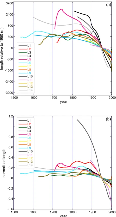
95 Fig 4. (a) Stacked glacier length records for the different regions; in (b) the corresponding normalised records are shown. Region numbers are shown in Fig. 2.

-3200 -2400 -1600 -800 0 800 1600 2400 3200

1500 1600 1700 1800 1900 2000

L1 L2 L3 L4

L5

L6

L7

L8 L9

L10 L11 L12 L13 L14

length relative to 1950 (m)

year

(a)

-0.6 -0.4 -0.2 0 0.2 0.4 0.6 0.8 1 1.2

1500 1600 1700 1800 1900 2000

L1

L2

L3 L4

L5 L6 L7 L8 L9 L10 L11 L12 L13 L14

normalised length

year

(b)

Fig. 4. (a) Stacked glacier length records for the different regions;

in (b) the corresponding normalised records are shown. Region numbers are shown in Fig. 2.

3 Stacked length records for regions

To get an impression of glacier changes on a regional scale, stacked records were constructed from all available data in a particular region. Figure 4 shows the stacked glacier length after smoothing once more with the Stineman-filter. This smoothing is necessary because jumps in the stacked record are created when a “new” record enters the stack or when a record in the stack ends. It is evident from Fig. 4 that the differences among the regions are significant, but all stacked records show glacier retreat after the mid-19th century. This again illustrates the coherency of the glacier signal over the globe.

96

96 Fig. 5. The stacked global glacier length signal. The dashed line shows the number of data points (after interpolation of the records) for individual years (scale on right). The other curves show

!

L (1,blue),

!

L 14 (2, red) and

!

L w14 (3, purple).

-500 0 500 1000 1500

0 50 100 150 200

1700 1750 1800 1850 1900 1950 2000

glacier length relative to 1950 (m)

number of records

year 1

2

3

Fig. 5. The stacked global glacier length signal. The dashed line

shows the number of data points (after interpolation of the records) for individual years (scale on right). The other curves show_L¯ _(1,

blue),L¯14(2, red) andL¯w14(3, purple).

In Fig. 4 there is a clear outlier: region 10 (Irian Jaya). The glaciers on Irian Jaya (Carstenz and Meren) have shown very strong relative retreats. But also the glaciers in central Africa (7 records) have become much smaller. It appears that the smallest relative changes have occurred in regions 3, 7 and 13 (S. Greenland/Iceland, Caucasus and Patagonia, respectively).

4 The global signal

It is clear that the majority of the records comes from re-gions where the ice cover is relatively small (notably the Alps and Rocky Mountains). The development of a globally-representative proxy for ice volume therefore requires a weighting procedure that reduces the relative effect of data-rich regions on the global signal. Here we achieve this by averaging the records of the 14 regions shown above. The result of this procedure is shown in Fig. 5.

The blue curve (1) in Fig. 5 refers to straighforward stack-ing of all available records (L)¯ . As mentioned above,L¯ is strongly biased towards the Alps, because about 30% of the records stems from this region. Giving equal weights to all regions (L¯14)then yields the red curve (2) in Fig. 5. The

differences betweenL¯ andL¯14 are not very large, although

the latter curve reveals a significantly larger glacier retreat during the period 1925–1975.

An other possible approach is to give different weights to the 14 regions, proportional to the glacierized areas in the regions (L¯w14). It can be argued thatL¯w14would be a

bet-ter proxy for total ice volume, because it removes the bias generated by more records in regions with smaller glaciers. The implication is that the signal is mainly determined by regions 1, 2, 3, 4 and 8 (see Table 1). It only makes sense to constructL¯w14for the period for which all these regions

J. Oerlemans et al.: Reconstructing the glacier contribution to sea-level rise 63 To obtain weighting factors, the glacierised area not

cov-ered within the 14 regions is added over the 14 regions (Table 1, column labelled “Addition”). In fact, this proce-dure reveals the weakness of the data set on glacier fluctua-tions, namely, that little is known in some regions with large amounts of ice. Admittedly, the partition of glacier area over the 14 regions is rather arbitrary. For instance, half of the glacier area in the Canadian arctic was added to region 1 (Alaska), and half to region 2 (Rocky Mountains). Simi-larly, the records from Jan Mayen and Svalbard (region 4) are supposed to represent all glaciers and ice caps in the Arc-tic ocean. However, we stress already at this point that in the end the weighting factors were not used in calculating the sea-level contribution from glaciers, because the weighted length curve is very similar to the unweighted curve.

In Fig. 5 it can be seen thatL¯w14 follows the same

pat-tern asL¯ andL¯14, but the amplitude of the signal is larger.

Records from regions 1, 2, 3, 4 and 8 are from glaciers larger than the average size in the dataset, and these tend to show larger fluctuations (presumably because the larger glaciers are flatter and therefore more sensitive to climate change, e.g. Oerlemans, 2005). It is therefore interesting to consider the normalised length records once more.

In analogy to the averaging procedure described above, ¯

L∗,L¯∗₁₄andL¯∗_w14have been calculated from the normalized length records (* refers to normalised). It should be noted that for a number of glaciersL1950 is not very well known

and has been obtained from interpolation on the nearest data points. However, this should hardly affect the results of the entire sample.

¯

L∗,L¯∗₁₄ and L¯∗_w14 are shown in Fig. 6. The curves ap-pear to be remarkably similar. This finding reflects the facts that (i) the behaviour of glaciers over the past few cen-turies has been coherent over the globe, and (ii) the rela-tive change in glacier length has not been very different for smaller and larger glaciers. Nevertheless, the normalisation brings out more clearly the maximum glacier size between 1825 and 1875, although it should be realised that the num-ber of records starting before 1850 is small (Fig. 5).

It would perhaps be most appropriate to base a proxy for changes in glacier volume on L¯∗_w14. This would unfortu-nately imply that one cannot go further back in time than around 1900. However, sinceL¯∗₁₄andL¯∗_w14are very similar, it should be possible to base an ice volume proxy onL¯∗₁₄. This will be worked out in the next section.

5 Towards a proxy for glacier volume

The next step to be made is to relate changes in glacier vol-ume to changes in glacier length. Although general scaling theories have been developed for this (e.g. Bahr et al., 1997), it is not a priori clear how these should be applied. It appears that for many glaciers the loss of volume is first of all the re-sult of a decreasing ice thickness and a decrease in area due

97 Fig. 6. As in Fig. 5 but now for normalized length records. The curves refer to

!

L *

(1,blue),

!

L 14* (2, red) and

!

L w14* (3, purple).

-0.1 0 0.1 0.2 0.3

1700 1750 1800 1850 1900 1950 2000

normalized glacier length relative to 1950

year 1

2

3

Fig. 6. As in Fig. 5 but now for normalized length records. The

curves refer to_L¯∗_{(1, blue),L}¯∗

14(2, red) andL¯

∗

w14(3, purple).

to a retreating glacier front. In many cases the adjustment of mean glacier width to a change in length is restricted by the geometry.

Here we use a relation that is in line with the scaling the-ory:

H Href

∝

L Lref

α

(2) whereH is mean ice thickness,Lglacier length or ice-cap radius and the subscript “ref” indicates a reference state. For a perfectly plastic glacier on a flat bed the mean thickness is proportional to the square root of the length, i.e.α=0.5 (Weertman, 1961). Numerical models, based on the shal-low ice approximation and integrated until steady states are reached, yield values in the 0.40 to 0.44 range, depending on the slope of the bed (Oerlemans, 2001; p. 69).

Next we write

V Vref

∝

L Lref

η

(3)

V denotes ice volume. Two extreme cases can be consid-ered. In the first case it is assumed that a change in glacier length will not affect the glacier width. The change in vol-ume is therefore only due to a change in mean thickness and a change in length, which implies thatη≈1.4 to 1.5. The second case refers to an ice cap which can move freely in all directions. The corresponding value of the exponent than isη≈2.4 to 2.5. These values ofηshould be compared to the scaling study of Bahr (1997). Based on the geometry of more than 300 glaciers, Bahr found that glacier area varies asL1.6; the corresponding value ofηwould be 2.0 to 2.1 (see also Barry, 2006).

Equation (3) refers to a single glacier. Now we postu-late that a similar approach can be applied to the normalised global glacier signalL¯∗₁₄:

64 J. Oerlemans et al.: Reconstructing the glacier contribution to sea-level rise

98

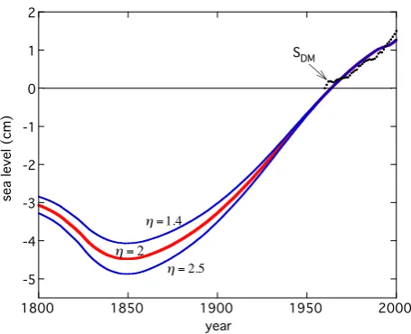
98 Fig. 7. Reconstruction of the glacier contribution to sea-level change for different values of η. The dots show the cumulative effect of global annual mass balance as calculated from observations by Dyurgerov and Meier (2005), see Fig. 1.

-5 -4 -3 -2 -1 0 1 2

1800 1850 1900 1950 2000

sea level (cm)

year

S_DM

!

"=2

!

"=2.5

!

"=1.4

Fig. 7. Reconstruction of the glacier contribution to sea-level

change for different values ofη. The dots show the cumulative ef-fect of global annual mass balance as calculated from observations by Dyurgerov and Meier (2005), see Fig. 1.

Note that according to this expression the nondimensional volume equals unity in the year 1950 for any value of the exponentη. V₁₄∗ is now considered to be the best possible glacier volume proxy derived from the set of glacier length records, withηwithin the 1.5 to 2.5 range, but probably close to 2.0.

One may argue that a more accurate proxy for glacier vol-ume could be obtained by estimating the volvol-ume of each in-dividual glacier in the sample. However, for larger values ofηthis leads to very large fluctuations because a few large glaciers may dominate the picture in an unrealistic way.

So far transient effects, i.e. an imbalance between the length and volume response to climate forcing, have not been considered. Experiments with numerical glacier models have been used to study characteristic response times for glacier length and volume (e.g. Greuell, 1992; Schmeits and Oer-lemans, 1997; OerOer-lemans, 2001; Leysinger Vieli and Gud-mundsson, 2004). In most studies it is found that glacier vol-ume adjusts somewhat more quickly to climatic forcing than glacier length. However, the difference in response time de-pends on the particular geometry and is generally small (typ-ically 10%, Van de Wal and Wild, 2001). Radic et al. (2007) carried out a more explicit test on the performance of volume scaling, paying attention to transient effects. They found that scaling is a powerful tool even when changes in the climatic forcing are relatively fast. In conclusion, we feel that de-tailed studies support the use ofV₁₄∗ as a proxy for changes in global glacier volume.

6 The glacier contribution to sea-level rise

To arrive at an estimate of the glacier contribution to sea-level change, V₁₄∗ is now calibrated with the compilation of mass balance data of Dyurgerov and Meier (2005), see Fig. 1. Dyurgerov and Meier (2005) estimated the change in glacier volume from mass-balance observations and ex-trapolated this to obtain an estimate of the annual contribu-tion of glacier shrinkage to sea-level change. We denote the cumulative contribution to sea-level change bySDM. Data

are used for the period 1961–2000 (the “learning period” for

V₁₄∗). The calibration is simply done by correlatingSDMand

V₁₄∗ for this period.

The correlation betweenSDMandV14∗ is high and mainly

stems from the linear trends during the period 1961–2000. Forη=1.4 the correlation coefficient is 0.944; forη=2 it is 0.938; forη=2.5 it is 0.936. On smaller time scales the re-lation betweenSDMandV14∗ is weaker. For instance, around

1990 the glacier contribution to sea-level rise calculated from

V₁₄∗ slightly declines, which is not seen inSDM. However,

one should realize that the set of glaciers for which length data are available is different from the set of glaciers on whichSDMis based.

After having calibratedV₁₄∗ withSDM, the glacier

contri-bution to sea-level can be extended backwards in time. Since the number of glacier records is small before 1800 and af-ter 2000, the result is only shown for the period 1800–2000. From Fig. 7 it is clear that the present estimate is large com-pared to numbers found in the literature: 5 to 6 cm for the period 1850–2000, 4 to 5 cm if the period 1900–2000 is con-sidered.

7 Discussion

Several test were carried out to see how sensitive the results are to the use of a different glacier length signal (e.g. deriving first hemispheric signals and then giving a larger weight to the Northern Hemisphere because the glacier area is much larger). It turns out that the sensitivity is small, which is a consequence of the rather coherent behaviour of glaciers over the globe (on a century time scale).

Figure 7 shows that the choice of the scaling parameterηis not very critical. A range of parameter values of 1.4 to 2.5 is really a wide range, yet the differences in the calculated sea-level contribution are within 1 cm for the period 1850–2000 [It should be noted that for every value ofηthe calibration with the mass-balance data is different].

We stress that the data on glacier area as summarized in Table 1 do not directly affect our estimate of the glacier con-tribution to sea-level rise. This information was only used to verify that L¯∗₁₄ can be used to construct a proxy for ice volume variations.

present approach is the assumption that bothSDM andL¯∗₁₄

are signals that are truly globally representative. An exten-sive discussion on SDM has been given in Dyurgerov and

Meier (2005). We note that the relative error in our estimate of the glacier contribution to sea-level rise is approximately proportional to the error in the glacier contribution calculated for the period 1961–2000. For instance, a 10% error would then imply a 0.5 cm error in the calculated glacier contribu-tion for the last hundred years. Altogether, our best esti-mates of the glacier contribution to sea-level rise are: for the period 1850–2000: 5.5±1.0 cm; for the period 1900–2000: 4.5±0.7 cm.

Compared to the number given in Zuo and Oerlemans (1997), namely 2.7 cm for the period 1865–1990, our cur-rent estimate is high. However, it should be remembered that the methodologies are quite different. In Zuo and Oerle-mans (1997) changes in glacier volume were calculated from modelled mass-balance sensitivities and observed tempera-ture data. Using glacier length records directly implies that all other effects (changes in precipitation, radiation, etc.) are implicitly included, although we still think that the tempera-ture effect is most important.

As noted before, the normalisation of the glacier length records brings out the 1850 maximum more sharply (com-pare Figs. 5 and 6). The implication is a clear minimum in the sea-level contribution around 1850 (Fig. 7). However, we note that the number of records in the first half of the 19th century is small. Consequently, the significance of the minimum should not be overestimated and we restrict our conclusions about the glacier contribution to sea-level rise to the period after 1850.

Edited by: A. Klein

References

Arendt, A., Echelmeyer, K., Harrison, W. D., Lingle, G., and Valen-tine, V.: Rapid wastage of Alaska glaciers and their contribution to rising sea level, Science, 297, 382–386, 2002.

Bahr, D. B.: Width and length scaling of glaciers, J. Glaciol., 43, 557–562, 1997.

Bahr, D. B., Meier, M. F., and Peckham, S. D.: The physical basis of glacier volume-area scaling, J. Geophys. Res., 102(B9), 20 355– 20 362, 1997.

Barry, R. G.: The status of research on glaciers and global glacier recession, Progr. Phys. Geogr., 30, 285–306, 2006.

Church, J. A. and White, N. J.: A 20t h century acceleration in global sea-level rise, Geophys. Res. Lett., 33, L01602, doi:10.1029/2005GL024826, 2006.

Dyurgerov, M. B. and Meier, M. F.: Glaciers and the changing earth system: a 2004 snapshot, Occasional Paper No. 58, INSTAAR, University of Colorado, 2005.

Greuell, W.: Hintereisferner, Austria: mass-balance reconstruction and numerical modelling of the historical length variations, J. Glaciol., 38, 233–244, 1992.

IPCC-2001, Climate Change 2001: The Scientific Basis Contribu-tion of Working Group I to the Third Assessment Report of the Intergovernmental Panel on Climate Change (IPCC), edited by: Houghton, J. T., Ding, Y., Griggs, D. J., Noguer, M., Van der Linden, P. J., and Xiaosu, D., Cambridge University Press, 2001. IPCC-2007, Climate Change 2007: The Physical Science Basis, Contribution of Working Group I to the Fourth Assessment Re-port of the IPCC, Cambridge University Press, http://www.ipcc. ch/, 2007.

Johannesson, T., Bj¨ornsson, H., and Grothendieck, G.: The Stinepack Package, Icelandic Meteorological Office, 2006. Kaser, G., Cogley, J. G., Dyurgerov, M. B., Meier, M. F., and

Ohmura, A.: Mass balance of glaciers and ice caps: Consen-sus estimates for 1961–2004, Geophys. Res. Lett., 33, L19501, doi:10.1029/2006GL027511, 2006.

Leysinger Vieli, G. J.-M. C. and Gudmundsson, G. H.: On estimating length fluctuations of glaciers caused by changes in climate forcing, J. Geophys. Res., 109, F01007, doi:10.1029/2003JF000027, 2004.

Meier, M. F.: Contribution of small glaciers to global sea-level, Sci-ence, 226, 1418–1421, 1984.

Oerlemans, J.: Glaciers and Climate Change, A.A. Balkema Pub-lishers, 2001.

Oerlemans, J.: Extracting a climate signal from 169 glacier records, Science, 308, 675–677, doi:10.1126/science.1107046, 2005. Radic, V., Hock, R., and Oerlemans, J.: Volume-area scaling

ap-proach versus flowline model in glacier volume projections, Ann. Glaciol., 46, 234–240, 2007.

Schmeits, M. J. and Oerlemans, J.: Simulation of the historical vari-ations in length of the Unterer Grindelwaldgletscher, J. Glaciol., 43(143), 152–164, 1997.

Rignot, E., Rivera, A., and Casassa, G.: Contribution of the Patag-onia Icefields of South America to global sea level rise, Science, 302, 434–437, 2003.

Stineman, R. W.: A consistently well-behaved method of interpola-tion, Creative Computing, July 1980, 54–57, 1980.

Van de Wal, R. S. W. and Wild, M.: Modelling the response of glaciers to climate change, applying volume-area scaling in com-bination with a high resolution GCM, Clim. Dyn., 18, 359–366, 2001.

Weertman, J.: Stability of ice-age ice-sheets, J. Geophys. Res., 66, 3783–3792, 1961.