The Cryosphere, 7, 1121–1137, 2013 www.the-cryosphere.net/7/1121/2013/ doi:10.5194/tc-7-1121-2013
© Author(s) 2013. CC Attribution 3.0 License.
EGU Journal Logos (RGB)
Advances in
Geosciences
Open Access
Natural Hazards
and Earth System
Sciences
Open AccessAnnales
Geophysicae
Open AccessNonlinear Processes
in Geophysics
Open AccessAtmospheric
Chemistry
and Physics
Open AccessAtmospheric
Chemistry
and Physics
Open Access DiscussionsAtmospheric
Measurement
Techniques
Open AccessAtmospheric
Measurement
Techniques
Open Access DiscussionsBiogeosciences
Open Access Open Access
Biogeosciences
DiscussionsClimate
of the Past
Open Access Open Access
Climate
of the Past
Discussions
Earth System
Dynamics
Open Access Open Access
Earth System
Dynamics
DiscussionsGeoscientific
Instrumentation
Methods and
Data Systems
Open Access
Geoscientific
Instrumentation
Methods and
Data Systems
Open Access DiscussionsGeoscientific
Model Development
Open Access Open Access
Geoscientific
Model Development
DiscussionsHydrology and
Earth System
Sciences
Open AccessHydrology and
Earth System
Sciences
Open Access DiscussionsOcean Science
Open Access Open Access
Ocean Science
DiscussionsSolid Earth
Open Access Open Access
Solid Earth
DiscussionsThe Cryosphere
Open Access Open Access
The Cryosphere
DiscussionsNatural Hazards
and Earth System
Sciences
Open Access
Discussions
Modelling and mapping climate change impacts on permafrost at
high spatial resolution for an Arctic region with complex terrain
Y. Zhang1, X. Wang2, R. Fraser1, I. Olthof1, W. Chen1, D. Mclennan3, S. Ponomarenko3, and W. Wu4
1Canada Centre for Remote Sensing, Natural Resources Canada, Ottawa, Ontario, K1A 0Y7, Canada
2College of Resources and Environmental Science, Hebei Normal University, Shijiazhuang, Hebei, 050024, China 3Parks Canada Agency, Hull, Quebec, K1A 0M5, Canada
4Western and Northern Service Centre, Parks Canada Agency, Winnipeg, Manitoba, R3B 0R9, Canada
Correspondence to: Y. Zhang ([email protected])
Received: 15 October 2012 – Published in The Cryosphere Discuss.: 6 November 2012 Revised: 21 May 2013 – Accepted: 15 June 2013 – Published: 18 July 2013
Abstract. Most spatial modelling of climate change
im-pacts on permafrost has been conducted at half-degree lat-itude/longitude or coarser spatial resolution. At such coarse resolution, topographic effects on insolation cannot be con-sidered accurately and the results are not suitable for land-use planning and ecological assessment. Here we mapped climate change impacts on permafrost from 1968 to 2100 at 10 m resolution using a process-based model for Ivvavik Na-tional Park, an Arctic region with complex terrain in northern Yukon, Canada. Soil and drainage conditions were defined based on ecosystem types, which were mapped using SPOT imagery. Leaf area indices were mapped using Landsat im-agery and the ecosystem map. Climate distribution was es-timated based on elevation and station observations, and the effects of topography on insolation were calculated based on slope, aspect and viewshed. To reduce computation time, we clustered climate distribution and topographic effects on in-solation into discrete types. The modelled active-layer thick-ness and permafrost distribution were comparable with field observations and other studies. The map portrayed large vari-ations in active-layer thickness, with ecosystem types being the most important controlling variable, followed by climate, including topographic effects on insolation. The results show deepening in active-layer thickness and progressive degrada-tion of permafrost, although permafrost will persist in most of the park during the 21st century. This study also shows that ground conditions and climate scenarios are the major sources of uncertainty for high-resolution permafrost map-ping.
1 Introduction
Climate warming at high latitudes was about twice the global average during the 20th century (ACIA, 2005). Observations have shown increases in near-surface ground temperature and active-layer thickness, and at some places, disappearance of permafrost (e.g., Vitt et al., 2000; Smith et al., 2010). Most climate models project that climate warming in northern high latitudes will continue at a rate higher than the global aver-age during the 21st century (ACIA, 2005), which will fur-ther induce permafrost degradation. Permafrost thaw affects infrastructure, ecosystems, wildlife habitats, and has strong feedbacks on the climate system (ACIA, 2005).
Fig. 1. (a) Relief map of Ivvavik National Park and summer thaw depth observation sites (red dots), and (b) location of the park. Green
squares are the locations of climate stations used in the study. The red dot in (b) is the location of Illisarvik in Richards Island.
resolution results are difficult to validate by comparing with field observations and are not suitable for land-use planning and for ecological assessment.
Modelling and mapping climate change impacts on per-mafrost at high spatial resolution requires detailed input data, efficient computation schemes, and robust models. Recently, several studies modelled permafrost at higher spatial reso-lutions. Jafarov et al. (2012) mapped ground thermal condi-tions and changes with climate in Alaska at 2 km resolution using an implicit finite-difference numerical model. The ef-fects of snow were considered explicitly but the topographic effect on solar radiation was not considered. Duchesne et al. (2008) mapped permafrost conditions and changes with climate in the Mackenzie basin at 30 m resolution based on a process-based heat conduction model. The model used sea-sonal n-factors to estimate the near-surface ground tempera-ture from air temperatempera-ture. Zhang et al. (2012, 2013) mapped permafrost in the northwestern Hudson Bay Lowlands at 30 m resolution using a more detailed model that integrated the effects of other climate variables (e.g. precipitation, so-lar radiation, and vapour pressure) and changes in snow and soil moisture conditions. This region mainly consists of a peatland plain, where peat layer thickness can be estimated based on elevation. However, Arctic regions are usually not flat and many factors affect the distribution of organic layer thickness. More importantly, complex terrain has significant effects on soil, vegetation, and local climate, and thus has high spatial variations in permafrost distribution. Therefore, higher spatial resolution is needed to map permafrost in com-plex terrain, especially for land-use planning and for assess-ing the impacts of permafrost on hydrology, ecosystems and geohazards. The objectives of this study are to develop an approach to model and map permafrost at high spatial reso-lution for an Arctic region with complex terrain, to test the
effects of spatial resolutions, and to identify the input data gaps for future studies.
2 Methods and data
2.1 The study area and field data sources
and status, ecosystem type, and summer thaw depth. Sum-mer thaw depth was measured at 162 sites across the park using steel probes and by digging soil profiles, of which 62 sites did not reach the frozen layer due to high stone content in the soil. Figure 1a shows the distribution of the 100 sites where summer thaw depths were recorded.
2.2 The model
The Northern Ecosystem Soil Temperature model (NEST) was used to compute and map permafrost conditions in the park. NEST is a one-dimensional transient model that siders the effects of climate, vegetation, snow, and soil con-ditions on ground thermal dynamics based on energy and mass transfer through the soil-vegetation-atmosphere sys-tem (Zhang et al., 2003). Ground sys-temperature is calculated by solving the one-dimensional heat conduction equation. The dynamics of snow depth, snow density and their ef-fects on ground temperature are considered. Soil water dy-namics are simulated considering water input (rainfall and snowmelt), output (evaporation and transpiration), and distri-bution among soil layers. Soil thawing and freezing, and as-sociated changes in fractions of ice and water, are determined based on energy conservation. Detailed descriptions of the model and validations can be found in Zhang et al. (2003, 2005, 2006). Lateral flows and snow drifting are parameter-ized in a simplified way (Zhang et al., 2002, 2012). We im-proved the model to address the topographic effects on inso-lation so that the NEST model could be used for areas with complex terrain. The algorithms are presented in Appendix A, and the source code is presented as Supplementary Mate-rial.
2.3 The input data and processing
2.3.1 Climate data
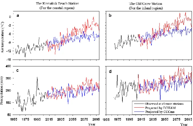
There are seven climate stations within or nearby INP. Three stations near the northern shoreline have about 50 yr of obser-vations while the other four stations, including all the three inland stations, have less than 15 yr of observations. Most of the data have some gaps. Several studies developed methods to spatially interpolate monthly climate based on station ob-servations (e.g., Wang et al., 2006; McKenney et al., 2011). Since temporal patterns are usually affected by the changes in climate stations with time used for the interpolation, we estimated the temporal patterns using observations at repre-sentative climate stations and estimated the average spatial distributions of air temperature and precipitation based on the monthly spatial data from Wang et al. (2006). Observa-tions show close correlaObserva-tions of air temperature among the stations in the park. For example, the correlation coefficient of the daily air temperature from 1968 to 2010 at Komakuk Beach Station (69.62◦N, 140.20◦W) and Old Crow Station (67.34◦N, 139.50◦W) is 0.92 (N=15706) although these
two stations are about 250 km apart across the park from the coast to inland (Fig. 1). The correlation of daily precipitation between these two stations is poor (R=0.16,N=15706). However, the monthly total precipitation is correlated be-tween the stations (R=0.50,N=516). Therefore we used station observed climate data to represent both the long-term patterns of the monthly climate and the daily fluctuations within a month for a region surrounding the climate station.
Monthly air temperature in a year for a grid cell was esti-mated by
Tm,g(Y, M)=T0 m,g(M)+1Tm,s(Y, M) (1) whereTm,g(Y, M)is the monthly mean air temperature for grid cell g in month M year Y. T0 m,g(M) is the 30 yr (1971–2000) mean air temperature in the monthM for the grid cellg, interpolated from climate stations based on Wang et al. (2006) using a spatial resolution of 30 m by 30 m (Fig. 2). 1Tm,s(Y, M) is the deviation of the monthly air temperature in yearY monthMfrom the 30 yr average for that month estimated based on the station observations. The daily air temperature for a grid cell was estimated based on the daily observations at a climate station
Td,g(Y, M, D)=Td,s(Y, M, D)+1Tm,gs(Y, M) (2) whereTd,g(Y, M, D) and Td,s(Y, M, D) are daily air tem-peratures (daily maximum or minimum) on day D month MyearY for a grid cell and a climate station, respectively. 1Tm,gs(Y, M)is the difference of monthly air temperatures between the grid cell and the climate station in month M yearY. Precipitation was estimated in a similar way but us-ing ratios instead of differences so that daily and monthly precipitation can be zero.
Fig. 2. Distribution of (a) mean annual air temperature, (b) mean annual total precipitation, (c) leaf area indices, and (d) ecosystem types
in Ivvavik National Park. Shaded relief was added for easy interpretation. The air temperature and precipitation were averages from 1971 to 2000 derived based on Wang et al. (2006). The leaf area indices were estimated based on Landsat imagery. The ecosystem map was from Fraser et al. (2012) (see Table 2 for the names of the ecosystem types).
respectively (Fig. 3). The monthly air temperature and pre-cipitation were converted to daily data using the above de-scribed method (Eqs. 1 and 2) based on the historical daily observations at climate stations.
Vapour pressure was estimated based on minimum air tem-perature (Zhang et al., 2012). Daily total insolation without topographic effects (an input to consider topographic effects on insolation as described in Appendix A) was estimated based on latitude, the day of the year, diurnal temperature range and vapour pressure (Zhang et al., 2012). The param-eters were estimated based on observations at Inuvik climate station (68.32◦N, 133.52◦W).
The coastal region of the park neighbours the Arctic Ocean and has a marine climate while the inland region has a con-tinental climate (Canadian Parks Service, 1993). We delin-eated the southern boundary of the coastal region based on the 300 m elevation contour. We used the daily climate ob-servations at Komakuk Beach Station and Old Crow Station to represent the temporal patterns of the climate in the coastal and the inland regions, respectively; as these two stations have the longest continuous observations within or nearby the park. Observations from these two stations are available
from 1958–2011 and 1968–2011, respectively. Data gaps are filled based on observations at nearby stations.
2.3.2 Classifying the average climate and topographic
effects on insolation
Since the spatial distributions of the climate were estimated based on long-term monthly means, which do not change with time, we discretized the average climate conditions of the grid cells into different clusters to reduce computation time. Permafrost conditions are mainly dependent on sea-sonal and annual climate conditions and are not very sen-sitive to day-to-day climate fluctuations. Active-layer thick-ness, for example, is mainly determined by the annual to-tal degree days when daily air temperature is above 0◦C (TDDT >0) according to the Stefan’s equation (Lunardini, 1981). Therefore we used TDDT >0and annual total precip-itation to cluster the average climate. The 30 m resolution TDDT >0and annual total precipitation were re-sampled to 10 m resolution using the nearest neighbour method.
Fig. 3. Changes of (a, b) annual mean air temperature and (c, d) annual total precipitation at the Komakuk Beach and Old Crow climate
stations. The observations at these two stations were used to represent the temporal patterns of climate in the coastal and the inland regions, respectively.
re-sampled from 30 m DEM data using bilinear interpolation method. We did this re-sample to match the resolution of the ecosystem map. The DEM data are from the Topographic Data Centre of Natural Resources Canada. The viewshed of a grid cell is the angular distribution of sky visibility ver-sus obstruction, similar to the view taken by upward-looking hemispherical (fisheye) photographs from the centre of the grid cell (Fu et al., 2000). Since most valleys in the park are less than 3 km wide between the peaks, we calculated view-shed for each 30 m by 30 m grid cell using a window of 201 by 201 grid cells of the DEM (or 3 km from the grid cell to the sides of the window). The viewshed angles were calcu-lated for each 22.5◦azimuth direction, with a total of 16 az-imuth directions for each grid cell. The viewshed angles were then interpolated to 10 m spatial resolution. Using slope, as-pect and the viewshed angles, average annual insolation was calculated for each grid cell for clustering analysis.
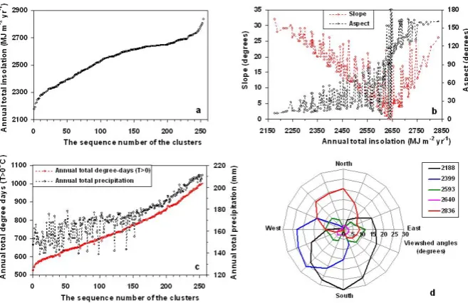
We clustered the average climate and topographic fea-tures based on TDDT >0, annual precipitation, average an-nual insolation, slope and aspect using PCI Isodata unsuper-vised classification method (PCI Geomatics Enterprises Inc. Canada). Since the software allows a maximum of 255 ters, we first clustered the inland region into nine large ters and then further clustered each of them into 254 ters. The coastal region was directly clustered into 254 clus-ters and the clustering errors were smaller than the errors for the inland region. Figure 4 shows an example of the climate, insolation and topographic conditions of the clusters in the coastal region. Table 1 lists the average clustering errors. The effects of the clustering errors on the active-layer thickness were generally less than 0.6 % based on Stefan’s equation.
To reduce the errors in estimated insolation for each clter, the topographic attributes of a cluster were assigned us-ing that of a grid cell within the cluster where the difference of the annual total insolation between the grid cell and the cluster average was the smallest. The latitude of that grid cell was used for calculating the insolation of that cluster as well. Similarly, monthly air temperature and precipitation of a cluster were assigned using that of a grid cell in the cluster where the difference of TDDT >0between the grid cell and the cluster average was the smallest.
2.3.3 Ecosystem types and distribution
Figure 2d shows the ecosystem types in INP mapped by Fraser et al. (2012) using 10 m-resolution SPOT imagery ac-quired during 13 July to 22 August 2006. The ecosystem types are described in Table 2. The map was developed using a new image-based predictive ecosystem mapping method, which integrates remote sensing-based vegetation map with predictive terrain attributes from a DEM (Fraser et al., 2012). A decision tree classifier was trained based on the ecosys-tem map of the Firth River basin, developed using air photos and detailed field observations at 367 sites by Mackenzie and MacHutchon (1996). The overall accuracy of the classifica-tion is 85 % (Fraser et al., 2012).
2.3.4 Ground conditions and hydrological parameters
Fig. 4. The conditions of the clusters in the coastal region. (a) annual total insolation of the clusters, (b) slopes and aspects of the clusters
corresponding to the annual total insolation of the clusters, (c) annual total degree days when air temperature is above 0◦C and annual total precipitation of the clusters, and (d) viewsheds of some selected clusters (the legend shows their corresponding annual total insolation (MJ m−2yr−1)). Aspect is 0◦for a slope facing north and it increases anti-clockwise. In (b), aspect was shown as 360 minus the aspect if it is larger than 180◦.
Table 1. The number of clusters and the average clustering errors for the inland and coastal regions.
The coastal The inland region region
Number of clusters 254 2286
Average errors in TDDT >0(degree days) 7.3 10.8 Average relative errors in TDDT >0(%) 1.0 1.2 Average relative errors in√TDDT >0(%)∗ 0.5 0.6 Average errors in TDDT <0(degree days) 54.6 133.7 Average relative errors in TDDT <0(%) 1.3 3.4 Average error in annual mean air temperature (◦C) 0.15 0.37 Average errors in annual total precipitation (mm) 5.6 10.3 Average relative errors in annual total precipitation (%) 3.4 4.1 Average errors in annual insolation (MJ m−2yr−1) 12.6 20.9 Average relative error in annual total insolation ( %) 0.2 0.4
Average errors in slopes (degrees) 0.9 1.8
Average errors in aspects (degrees) 3.1 8.4
∗According to Stefan’s equation, active-layer thickness is proportional to√TDD
T >0. TDDT >0and TDDT <0 are annual total degree days for daily air temperature above and below 0◦C, respectively.
soils, fraction of gravel (from pebbles to boulders), lateral inflow and outflow parameters, and the snow-drifting pa-rameter. Since no detailed maps are available for these in-put data, we estimated their spatial distributions based on the ecosystem map. For each ecosystem type, the texture of the mineral soil was determined based on the typical con-ditions reported by Mackenzie and MacHutchon (1996) and our field observations (Table 3). Peat thickness was estimated based on our field measurements and the land features of the types, especially the drainage and moisture regime described
Table 2. The biophysical groups and ecosystem types in
Iv-vavik National Park. More detailed descriptions of the terrain fea-tures, vegetation compositions, and soil conditions can be found in Mackenzie and MacHutchon (1996).
Biophysical Type Ecosystem types groups codes
Alpine slopes 1 Alpine slope 2 Rock – lichen
Nivation and 3 Heather – bearflower nivation slope seepage slopes 4 Alder – heather seepage slope
5 Birch – crowberry mesic slope
Dry to moist 6 Willow – birch moist slope mountain slopes 7 Spruce – kinnikinnick dry slope
8 Spruce – birch mesic slope
Wet mountain 9 Spruce – horsetail wet slope slopes 10 Willow – horsetail wet slope
Drainage 11 Coltsfoot – mountain sorrel drainage area channels 12 Willow – coltsfoot drainage channel
13 Alaska willow drainage channel
14 Cotton – grass tussock Pediment 15 Alder – cotton-grass tussock slopes 16 Sedge tussock
17 Willow – sedge pediment drainage channel
Inactive alluvial 18 Hedysarum-avens inactive alluvial Terrace terraces 19 Willow inactive alluvial terrace
20 Spruce – rhododendron inactive alluvial terrace
Wetlands 21 Graminoid wetland 22 Dupontia marsh
23 Forb floodplain Active 24 Willow floodplain floodplain 25 Cottonwood floodplain
26 Sand and silt bars
water. The thickness of the subsoil was estimated assuming that the fraction of gravel increases 2 % for every 10 cm until the gravel fraction reaches 100 %. The ground conditions for the ecosystem types were listed in Table 3.
Lateral flow parameters were estimated based on the drainage class and moisture regime of the ecosystem types reported by Mackenzie and MacHutchon (1996) (Table 3). We assumed that the lowest water table depth for lateral out-flow (ranged from 0 m to 0.4 m) is proportional to the soil moisture class (ranging from 0 to 8 representing moisture regimes from hydric to very xeric), and the rate of lateral outflow is exponentially related to the drainage class number (ranging from 0 to 6 representing drainage types from very poor to very rapid). We also assumed that there is no surface lateral inflow and water will flow away gradually when the water table is above the land surface (water table decreases 5 % each day when it is above the land surface).
The snow-drifting parameter was estimated considering the effects of land exposure, plant forms and density. We de-fined the land exposure of a grid cell based on the typical terrain features of the ecosystem types described by Macken-zie and MacHutchon (1996). We divided vegetation into six
plant forms (coniferous trees, deciduous trees, medium to tall shrubs (≥0.5 m), low shrubs (<0.5 m), sedges or grasses with low shrubs, and sedges or grasses). The effects of plant density were estimated based on leaf area indices (LAI).
Since geothermal observations were sparse in Arctic re-gions, all the grid cells in the park were assumed to have the same geothermal heat flux (0.08 W m−2)and the same ther-mal conductivity for the bedrock (2.28 W m−1◦C−1), esti-mated based on site observations (Pollack et al., 1993; Jessop et al., 1984; Majorowicz et al., 2004).
2.3.5 Leaf area indices
Leaf area index was downscaled to 10 m spatial resolution using the 30 m resolution foliage biomass from Landsat im-agery
L10 m, i=9B0(Ei)·S (Ei)·B30 m
9
X
j=1
B0 Ej Ej (3)
whereL10 m, i is the estimated LAI for a 10 m pixeli (cm2 leaf cm−2land),Ei andEj are the ecosystem types for the 10 m pixelsi andj, respectively.j ranges from 1 to 9 for the nine 10 m pixels in the 30 m Landsat pixel.B30 m is the foliage biomass of the 30 m pixel (g cm−2). B30 m is cal-culated using a regression equation of simple ratio vegeta-tion index (band-4/band-3) of Landsat imagery (acquired on 30 August 2001) (Chen et al., 2013).B0(Ej)is the average foliage biomass (g cm−2)for an ecosystem typeEj, which was estimated as the average of all the 30 m pixels in the park whereEj is the dominant ecosystem type.S(Ei)is the spe-cific leaf area (cm2g−1)of the ecosystem type (122 cm2g−1 for sedges; 154 cm2g−1for deciduous shrub; 74 cm2g−1for evergreen shrubs; and 50 cm2g−1for black spruce) (Kattge et al., 2011). Some steep areas were blocked by shadows in the Landsat imagery. We estimated LAI in these areas as the average LAI of the ecosystem type B0(Ei)S(Ei). Fig-ure 2c shows the distribution of LAI in the park. LAI was discretized into 18 classes (increasing exponentially from 0 to 4.0) in modelling.
2.4 Computation procedure
Table 3. Ground conditions defined for each ecosystem type.
Type Drainagea Moistureb Sitesc Org. layer (cm)d Soil textureg SOM Gravel
codes (%)j (cm, %)k
Ob.e Def.f Ob.h Def.i
1 4–5 1–2 19 0–15 5 S, L, S S 10 0, 10-5LAI
2 5 1 8 0–5 5 S, Si, L S 10 0, 20-5LAI
3 3 3–4 3 4 4 SL SL 20 30, 10
4 3–5 4-5 0 – 4 – SL 20 30, 10
5 3–4 2–4 8 0–3 0 S, L, Si L 20 30, 5
6 2–4 4–5 8 0 0 L, Si L 80 40, 5
7 3–5 2–3 2 2–5 0 L, LS L 50 30, 5
8 3 3–5 10 5–30 10 S, Si, SiL Si 20 30, 5
9 1–3 5–6 10 0–20 10 Si Si 20 40, 5
10 1–3 5–7 16 0–40 5 Si, SiC, SiC Si 20 40, 5
11 2–3 5 2 4 4 L L 10 0, 10
12 2–3 5 1 5 5 SCL, SiCL, C SiCL 10 10, 5
13 1–2 4–5 3 0–12 5 Si, SiL, C SiL 10 10, 10
14 1–2 5–6 5 10–30 30 Si, C Si 50 40, 5
15 2–3 5 1 10 10 – Si 30 30, 5
16 2–3 5–7 10 10–29 20 Si, L Si 15 30, 5
17 1–2 6–7 5 0–19 10 S, Si, L S 20 30, 5
18 4–5 1–3 0 – 0 SL, LS SL 10 30, 5
19 3–5 2–3 3 0–10 5 S, Si Si 10 30, 5
20 3–5 2–3 12 0–21 10 Si, S, SL Si 20 30, 5
21 0–1 7–8 19 10–>40 30 Si, SiL, C SiCL 5 50, 5
22 0 7–8 0 – 0 – S 30 20, 5
23 6 7 0 – 0 – S 20 40, 30
24 4 4–5 3 0–5 5 S S 20 40, 30
25 4 4–5 5 2–14 8 S, L L 10 40, 30
26 4 4–5 0 – 0 – S 2 30, 10
aDrainage classes 0 to 6 represent very poorly, poorly, imperfectly, moderately well, well, rapidly, and very rapidly, respectively, defined based on Agriculture Canada Expert Committee on Soil Survey (1987). The data were from Mackenzie and MacHutchon (1996).
bSoil moisture regimes 0 to 8 represent very xeric, xeric, sub-xeric, sub-mesic, mesic, sub-hygric, hygric, sub-hydric, and hydric, respectively, defined based on Walmsley et al. (1980). The data were from Mackenzie and MacHutchon (1996).
cThe number of sites observed during 2008–2011 for estimating the ground conditions. dThe top organic layer thickness.
eObserved range of top organic layer thickness during 2008–2011. fThe top organic layer thickness defined for the model input.
gSoil texture symbols are S for sand, L for loam, Si for silt, and C for clay.
hObserved soil texture was from Mackenzie and MacHutchon (1996) and from our fieldwork during 2008–2011. iThe soil texture defined for the model input.
jThe soil organic matter content in the top mineral soil. It was defined based on observations during 2008–2011.
kThe depth (cm) where gravels first appears and the content of the gravel (%) at this depth. Gravel content gradually increases with depth after this layer. The data were estimated from Mackenzie and MacHutchon (1996) and our fieldwork during 2008–2011.
time was reduced significantly for this high-resolution spatial modelling.
The daily climate data observed at the Old Crow and Ko-makuk Beach stations were from 1968 and 1958, respec-tively. For spatial consistency, we modelled the permafrost in the park from 1968. To initialize the model, we selected the daily climate data in a year (1972 and 1964 for the Old Crow and Komakuk Beach stations, respectively) which had a climate close to the climate extrapolated for the year 1967. We ran the model iteratively using these years’ climate un-til the modelled ground temperature was stable, then ran the model from 1968–2011 based on the observed daily climate.
After that, we ran the model for the two climate scenarios to 2100.
3 Result and analysis
3.1 Spatial distribution of active-layer thickness
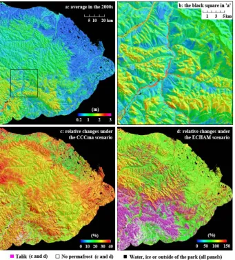
Fig. 5. Modelled distribution of (a) average active-layer thickness in the 2000s (i.e., 2000–2009), (b) an enlarged area for the black square in (a), and relative changes of active-layer thickness from the 2000s to the 2090s under the climate scenarios of (c) CCCma and (d) ECHAM.
Shaded relief was added for easy interpretation.
A thicker active layer was evident in the upper mountains and along drainage channels in some valleys. The results also show significant differences among ecosystem types (Fig. 6c). Alpine slopes and rock-lichen areas had thick ac-tive layers because they have no organic layer on the surface and usually contain high fractions of gravels in the soil. Ac-tive floodplains (types 23–26) and drainage channels (types 11–13) had thicker active layer as well due to their wet condi-tions and high gravel content. Pediment slopes (types 14–17) and graminoid wetland (type 21) had thin active layer due to the thick peat layer and wet conditions.
We calculated the average active-layer thickness for each climate-topography cluster (Fig. 6). The results show that the average active-layer thickness increased steadily with sum-mer air temperature. Figure 6a also shows a slightly different trend for the coastal region, where the active layer was thin-ner due to the peaty and wet soil conditions in this region.
Active-layer thickness also increased slightly with annual in-solation (Fig. 6b), but the correspondence is scattered due to the effects of other factors, especially the ecosystem types and air temperature. Active-layer thickness decreased with LAI due to the shading effects of plants (Fig. 6d).
Fig. 6. Correspondence of the modelled average active-layer thickness in the 1970s to (a) the average summer air temperature
(June–September), (b) annual solar radiation, (c) ecosystem types, and (d) leaf area indices. The range bars in (c) and (d) are the aver-age absolute deviations within the classes.
Table 4. The average absolute intra-class deviation and the
aver-age absolute inter-class deviation of the active-layer thickness in the 1970s calculated based on the ecosystem types, climate-topography clusters, and LAI classes.
Ecosystem Climate- LAI types topography classes clusters
Number of types or classes 26 2540 18
Averages of the classes without considering the size of the land areas
Average inter- (m) 0.21 0.14 0.09
class deviation (%)∗ 27.6 20.5 12.5
Average intra- (m) 0.15 0.16 0.19
class deviation (%)∗ 19.2 22.6 28.2
The ratio between inter-class
and intra-class deviations 1.43 0.91 0.44
Weighted averages based on the fraction of the land area of the classes
Average inter- (m) 0.28 0.23 0.24
class deviation (%)∗ 39.9 32.6 33.5
Average intra- (m) 0.13 0.18 0.20
class deviation (%)∗ 18.3 25.5 27.9
The ratio between inter-class
and intra-class deviations 2.18 1.28 1.20
∗In percentage of the average active-layer thickness of the type or class.
climate-topography clusters, and then by LAI classes. This result indicates that ecosystem type was the most important factor differentiating the modelled active-layer thickness in the park whereas LAI was the least important factor. When the averages were weighted by the land areas of the classes, ecosystem type was still the most important factor
control-ling the spatial distribution of active-layer thickness in the park. The importance of the LAI was close to that of the climate-topography because the variation of LAI was asso-ciated with the ecosystem type and climate. Ecosystem type was the dominant factor mainly because the corresponding ground conditions are the most important factor controlling active-layer thickness in this region (Wang et al., 2010).
3.2 Changes in active-layer thickness and permafrost
distribution
Fig. 7. Changes in active-layer thickness and degradation stages. (a) Mean active-layer thickness. (b) and (c) are the percentages of
land areas in different degradation stages in the park under the cli-mate change scenarios of CCCma and ECHAM, respectively. The degradation stages are based on Zhang (2013).
With progressive deepening in summer thaw depth, the deep layer thawed in summer may not be frozen back in the following winter, thus forming a year-round unfrozen layer, called talik, between the permafrost and the seasonal thaw-ing/freezing layer. Currently permafrost underlies almost all the land areas in the park and very small areas contain taliks (in the 2000s, the land area with taliks and the area with-out permafrost in the park accounted for only 0.0007 % and 0.004 %, respectively). From the mid-21st century, more ar-eas were predicted to develop taliks and permafrost
disap-peared in some southern areas. By the end of the 21st cen-tury, taliks developed in 0.1 % and 13.7 % of the land area in the park under CCCma and ECHAM, respectively, and per-mafrost disappeared in 2.1 % and 5.2 % of the area in the park under these two scenarios. Talik development occurred mainly in the southern areas of the park (Fig. 5c and d). Taliks could develop in most of the ecosystem types, except in pediment slopes and graminoid wetland. Permafrost could disappear in forests and in some southern valleys, mainly in floodplains and inactive alluvial terraces.
3.3 Permafrost degradation stages
Zhang (2013) divided permafrost degradation process in-duced by climate warming into five stages: gradual-thawing stage, increased-gradual-thawing stage, frequent-talik stage, isothermal-permafrost stage, and permafrost-free stage. We determined the stages for each grid cell in the park based on the model results. From 1967 to 2011, 8.7 % of the per-mafrost area in the park transferred from gradual-thawing stage to the increased-thawing stage, with very small ar-eas (<0.01 %) in frequent-talik and permafrost-free stages (Fig. 7b). By the end of the 21st century, the model pre-dicted that more areas would be in higher degradation stages, although significant differences existed between the two climate scenarios. Under scenario CCCma, the area with gradual-thawing permafrost would be reduced to 84.8 % of the area in INP by the end of the 21st century, while the area with increased-thawing stage and permafrost-free area would expand to 12.8 % and 2.1 % of the area in INP, re-spectively. More significant degradation was predicted under the ECHAM scenario. By the end of the 21st century, only 19.9 % of the area in INP would contain gradual-thawing permafrost. Permafrost in increased-thawing stage would expand to 53.0 % of the area in INP. Permafrost in other degradation stages would also expand under this scenario (Fig. 7). Spatially, permafrost in increased-thawing stage and permafrost-free areas are mainly located in some valleys and south-facing slopes under scenario CCCma. Under scenario ECHAM, most of the northern area in the park would be in increased-thawing stage while most of the southern area would be in frequent-talik and isothermal-permafrost stages, and some areas would be permafrost free.
3.4 Comparison with observations and results from
other studies
Fig. 8. Comparison between the modelled and measured summer
thaw depth. The model significantly over-estimated the seven sites in the circle, which are rock-lichen and alpine slopes, probably due to spatial heterogeneity or mistaking rocks for frozen ground. The solid line corresponds to the linear regression equation shown in the panel. The dashed line is a 1-to-1 line for reference.
thaw depths at these sites are probably due to local variations in soil conditions or mistaking rocks for frozen ground. Sum-mer thaw depths greater than one meter were observed in some alpine slopes although most observations did not reach the frozen layer (therefore they are not included in Fig. 8). Model tests also suggested that the active layer was thick in alpine slopes due to lack of organic layer, high gravel con-tent and sparse vegetation (Wang et al., 2010). The corre-lation coefficient between the modelled and observed sum-mer thaw depth is low (R=0.56,N=93), even excluding the seven sites. The low correlation is mainly due to varia-tions of ground condivaria-tions within an ecosystem type. There-fore, more spatially detailed maps for ground conditions are needed for high-resolution mapping of permafrost.
Based on field observations, Tarnocai (1986) created a polygon map of active-layer thickness for the INP area. The mapped median active-layer thickness is 0.4 m (0.3–0.5 m) in most northern coastal regions and 0.75 m (0.7–1.0 m) in the northern deltas. The median active layer is 0.7 m (0.5–0.9 m) along the large valleys and 1.35 m (0.5–2 m) in inland moun-tain regions. This spatial pattern and the range of the active-layer thickness are similar with our modelled results although his map was represented by only 15 polygons within the park. The modelled permafrost in this region is continuous, which is in agreement with the permafrost map of Canada (Heginbottom et al., 1995). The modelled permafrost thick-ness ranged from 150 m to 300 m, which is similar with the observations in this region (Smith and Burgess, 2002).
Fig. 9. Comparison between the modelled active-layer thickness in
the coastal region and measured summer thaw depth at Illisarvik in Richards Island (1983–2012. The circles) and in Herschel Island (2003–2007. The filled squares). The measurements at Illisarvik in Richards Island during 1983–2008 are from Burn and Kokelj (2009), and the unpublished data during 2009–2012 are kindly pro-vided by Christopher Burn. The measurements in Herschel Island are from Burn and Zhang (2009). The modelled active-layer thick-ness in 2012 is the average modelled based on the two climate sce-narios for that year.
Fig. 10. The modelled spatial distributions of active-layer
thick-ness (averages during the 2000s) at different spatial resolutions for a 20 km by 20 km area. The spatial resolutions are indicated in (a–g). The location of the area in the park (the red square) is shown in (h). To show the difference between (a) and (b), a small area (the black squares in (a) and (b)) was enlarged and shown in (d) and (e).
Burn and Zhang (2009) also measured summer thaw depth in Herschel Island from 2003 to 2007. Its magnitude and inter-annual fluctuations are comparable with our modelled active-layer thickness except in 2007, in which the observa-tion shows a significant increase (The squares in Fig. 9). Burn and Kokelj (2009) reported a long-term record of summer thaw depth since 1983 measured at Illisarvik in Richards Is-land (69.48◦N, 134.59◦W) (The red dot in Fig. 1b), probably the longest continuous measurements of summer thaw depth available. The modelled active-layer thickness is closely correlated with these measurements (R=0.71,N=30) al-though the absolute values are somewhat different due to the differences in climate and ground conditions between the observation sites and the coastal region in INP (Fig. 9). The modelled deepening trend of active-layer thickness was 2.9 cm per decade from 1983 to 2012, which was similar to that of the observations (deepening 2.3 cm per decade).
4 Discussion
This study mapped permafrost distribution and changes with climate in an Arctic region with complex terrain at 10 m spa-tial resolution using a process-based model. Compared to previous studies, several features of this work are notewor-thy. First, this study used a higher spatial resolution than pre-viously published modelling and mapping work, such as the
Fig. 11. The effects of spatial resolution on the modelled
active-layer thickness for a 20 km by 20 km area shown in Fig. 10h. The average is calculated for all the grid cells in the area during 1967–2100. The spatial standard deviation was calculated based on all-year averages (1967–2100) of the grid cells. The future years (2012–2100) was modelled based on scenario ECHAM. The pat-terns are very similar using the scenario CCCma.
30-m resolution modelling studies (Duchesne et al., 2008; Zhang et al., 2012), the 2 km-resolution study (Jafarov et al., 2012), or the half-degree latitude/longitude or even coarser resolution modelling studies (Zhang et al., 2006, 2008). In this high-resolution study, satellite remote sensing data were used more effectively; topographic effects on solar radiation can be calculated more accurately; the plot size of field ob-servations (large uniform plots are usually hard to find in re-gions with complex terrain) is comparable to the grid size, therefore they can be used directly for model calibration and validation; and the results reveal more spatial details, and are therefore more suitable for land-use planning and ecological monitoring and assessment.
Secondly, although several studies have mapped per-mafrost in mountainous regions at high spatial resolution and considered topographic effects on insolation (e.g., Bon-naventure et al., 2012), they assumed that permafrost condi-tions are in equilibrium with climate (see reviews by Rise-borough et al., 2008). Ground temperature observations and modelling studies have shown that the current and future permafrost conditions are not in equilibrium with the atmo-spheric climate (Osterkamp, 2005; Zhang et al., 2008). The modelled talik development and different degradation stages in this study are examples of the disequilibrium response of permafrost to climate change.
Thirdly, although permafrost will persist in most of the park in the 21st century, the model results show changes in permafrost degradation stages with climate warming. Com-pared to fluctuating active-layer thickness, the degradation stages clearly categorized the degradation processes of per-mafrost with climate change (Fig. 7). Our sensitivity tests also show that the effects of snow conditions on active-layer thickness were dependent on degradation stages. When per-mafrost is in the gradual-thawing stage, changes in snow drifting condition had almost no effects on active-layer thick-ness. When permafrost is in increased-thawing stage or taliks developed, reducing snow drifting (i.e., with deeper snow ac-cumulated) would increase summer thaw depth.
And finally, this study estimated daily climate variations based on station observations and used a clustering method to consider climate distribution and topographic effects on insolation. The estimated climate is directly linked to sta-tion observasta-tions and the clustering approach significantly reduced computation time for high-resolution spatial mod-elling. Such methods could be useful for other process-based high-resolution spatial modelling, such as for ecological and biogeochemical processes.
This study also indicates several sources of uncertain-ties or information gaps for permafrost mapping. One major source of uncertainty is the information about ground con-ditions. Although satellite data now can provide high spatial resolution maps for land cover and vegetation conditions, soil maps are still very coarse, especially for Arctic regions. We estimated soil and drainage conditions based on ecosystem types. Soil and drainage conditions, however, could differ widely within an ecosystem type. Therefore the results can only represent permafrost conditions under typical ground conditions of the ecosystem types. Improving the informa-tion about soil and drainage condiinforma-tions is important not only for permafrost mapping but also for other applications, such as ecosystem assessment and infrastructure development un-der a changing climate. Another major uncertainty is the fu-ture climate. The results of this study show significant dif-ferences in projected permafrost conditions under the two climate scenarios. Under the warmer scenario ECHAM, the projected changes in active-layer thickness not only showed a larger increase but also with a wider range of fluctuation, and the areas with taliks or even disappearance of permafrost
are much larger than that of the cooler scenario CCCma. The sparse and relatively short climate records in Arctic regions also affect the accuracy of the model results. The climate of the first year selected to initialize the model could affect the simulated permafrost thickness and the long-term trends of ground thermal conditions.
Although we considered snow drifting and lateral wa-ter flows, the NEST model is still one-dimensional, assum-ing each grid cell to be uniform and the lateral heat flux can be ignored. Therefore the results do not represent ar-eas with strong lateral heat fluxes, such as sharp mountain peaks or edges, and the areas very close to waterbodies. Cli-mate change and fire disturbances have significant impacts on vegetation conditions and LAI, which will affect per-mafrost through their effects on snow drifting and energy ex-changes between the land surface and the atmosphere. In this study, however, we did not consider changes in LAI caused by disturbances or plant growth with climate change. Our sensitivity tests suggest that increasing LAI without changes in the snow drifting factor will reduce active-layer thickness due to shading effects. Reducing snow drifting or even cap-turing some snow from surroundings will cause faster thaw-ing from the bottom of permafrost. Its effects on active-layer thickness depend on the stages of permafrost degradation. Therefore changes in vegetation and associated snow drift-ing could affect permafrost conditions in different ways.
5 Conclusions
of the region during the 21st century. This study also shows that ground conditions and climate scenarios are the major sources of uncertainty for high-resolution permafrost map-ping.
Appendix A
Calculating topographic effects on insolation
Topography affects insolation due to slope and aspect of the local land surface and the shading effects of the surrounding mountains and hills. The shading effect was calculated based on the viewshed approach (Fu and Rich, 2000). A viewshed is the angular distribution of sky obstructed by the surround-ing mountains and hills, similar to the view taken by upward-looking hemispherical (fisheye) photographs. The maximum obstruction angle in an azimuth direction can be determined based on the distance and elevation of the cells in that direc-tion.
Viewshed affects both direct and diffuse solar radiation. The diffuse solar radiation accepted by a grid cell can be cal-culated by
Rdiff=Rdiff0·Fdiff,topo (A1) whereRdiff is the diffuse solar radiation accepted in a grid cell.Rdiff0is the diffuse solar radiation accepted on a surface without obstructions from surroundings (W m−2).Fdiff, topo is the relative diffuse radiation received in the grid cell com-pared to a grid cell without surrounding obstructions (a ratio). If we assume that diffuse solar radiation is from sky only, the entire hemisphere is in isotropic distribution (Goudriaan, 1977), and omit the effects of slope and aspect on diffuse radiation,Fdiff, topocan be estimated as
Fdiff, topo= 1 π 2π Z 0 π/2 Z v(α)
sinβ·cosβ·dβ·dα (A2)
whereαis the azimuth direction, andβis the elevation angle (referring to the horizontal surface), and v(α)is the maxi-mum elevation angle obstructed by the surrounding moun-tains and hills in the directionα.
Direct solar radiation accepted in a grid cell at a time can be calculated by
Rdir=
Rdir0·[cosθ·cosGs+sinθ·sinGs·cos(α−Ga)] cosθ [θ <0.5π−v (α)]
0 [θ≥0.5π−v (α)]
(A3)
whereαandθ are the azimuth and zenith angles of the sun at the time. They can be determined based on latitude, day of year, and the time of day.Gs andGa are the slope and aspect of the surface of the grid cell.Rdir0is the direct solar radiation accepted on a horizontal surface without obstruc-tion from the surroundings (W m−2). The relative effects of
topography can be expressed as
Fdir, topo=
[cosθ·cosGs+sinθ·sinGs·cos(α−Ga)]
cosθ [θ <0.5π−v (α)] 0 [θ≥0.5π−v (α)]
(A4)
whereFdir, topois the relative effects of topography on direct solar radiation. The irradiance received in a grid cell at any time of day is the sum of the direct and diffuse solar radiation received in that grid cell.
It is difficult and usually unnecessary for the users to pro-vide hourly climate data for long-term permafrost modelling although they are needed for energy balance computation. Therefore we estimated the diurnal variations of both direct and diffuse solar radiation for each day using cosine func-tions based on Wang et al. (2002)
Rdir0=Rday0 1−Fdiff0, dayF1, θ n·Fdir, topo ·cos
θ−θ n
π/2−θ n· π 2
cosθ
cosθ n (A5)
Rdiff0=Rday0·Fdiff0, day·F2, θ n·Fdiff, topo
·cos
θ−θ n
π/2−θ n· π 2
(A6) whereθnis the zenith angle of the sun at noon (in radians) on that day,F1, θ nis the ratio between direct solar radiation at noon and the daily mean direct solar radiation on a horizontal surface, andF2, θ nis the ratio between diffuse solar radiation at noon and the daily mean diffuse solar radiation on a hori-zontal surface.Rday0 is daily average insolation received on a horizontal surface (W m−2), andFdiff0, day is the fraction of daily diffuse solar radiation in the daily total insolation received on a horizontal surface.Rday0can be calculated by
Rday0=106Rday00 /D (A7)
whereRday00 is the daily total insolation received on a hor-izontal surface (MJ m−2d−1), which is the input for the model.Dis day length (s) determined based on latitude and the day of the year.
Wang et al. (2002) developed regression relationships to determineF1, θ n andF2, θ n based on θn for a location. Our numerical simulation showed that the relationships change with latitude, especially when the day length reaches 24 h. Therefore we determined F1, θ n and F1, θ n numerically for each day of the year based on the original equations from Wang et al. (2002).
F1, θ n=D
D Z 0 cos
θ−θ n
π/2−θ n· π
2
cosθ
cosθ ndt
−1
(A8)
F2, θ n=D
D Z 0 cos
θ−θ n
wheret is time (s). The daily fraction of diffuse radiation in daily irradiance received on a horizontal surface (Fdiff0, day) can be estimated using a logistic function based on Boland et al. (2008). We slightly modified the parameters based on the daily insolation data observed at Inuvik climate station (68.32◦N, 133.52◦W)
Fdiff0, day=
1.05
1+exp(−4.5+8.6F0)
(F0>0.175) 1.0 (F0≤0.175)
(R2=0.715, N=13 209) (A10)
whereF0is the ratio of daily irradiance received on a hori-zontal surface to the daily irradiance on the top of the atmo-sphere.R2is the square of the correlation coefficient, and N is the number of valid daily data during 1959–2005 at Inuvik climate station from Environment Canada and the National Research Council of Canada (2007). Daily irradiance on the top of the atmosphere can be calculated by
R0, atm=10−6Sc D
Z
0
cosθdt (A11)
whereR0, atmis daily irradiance on the top of the atmosphere (MJ m−2d−1), Sc is the solar constant (W m−2).
The source code (in C++) for implementing these algo-rithms was provided as Supplement.
Supplementary material related to this article is available online at: http://www.the-cryosphere.net/7/ 1121/2013/tc-7-1121-2013-supplement.pdf.
Acknowledgements. The authors would like to thank Ying Zhang and Sergey Samsonov for their critical internal review of the paper. Thanks are also given to Christopher Burn for his comments and field data for validating the results. The comments from the two anonymous reviewers were very helpful in improving the quality of the paper. This study was supported by the Canadian Space Agency under the ParkSPACE GRIP project and by Natural Resources Canada under the Remote Sensing Science Program (Earth Science Sector contribution number 20120211).
Edited by: T. Zhang
References
ACIA: Impact of a Warming Arctic: Arctic Climate Impact Assess-ment. Cambridge University Press, 1042 pp., 2005.
Agriculture Canada Expert Committee on Soil Survey: The Cana-dian System of Soil Classification, 2nd Edn., Agriculture Canada, Publication 1646, Ottawa, Canada, 164 pp., 1987. Anisimov, O. and Reneva, S.: Permafrost and changing climate: The
Russian perspective, Ambio, 35, 169–175, 2006.
Boland, J., Ridley, B., and Brown, B.: Models of diffuse solar radi-ation, Renew. Energ., 33, 575–584, 2008.
Bonnaventure, P. P., Lewkowicz, A. G., Kremer, M., and Sawada, M. C.: A permafrost probability model for the southern Yukon and northern British Columbia, Canada, Permafrost Periglac., 23, 52–68, doi:10.1002/ppp.1733, 2012.
Burn, C. R. and Kokelj, S. V.: The environment and permafrost of the Mackenzie Delta area, Permafrost Periglac., 20, 83–105, doi:10.1002/ppp.655, 2009.
Burn, C. R. and Zhang, Y.: Permafrost and climate change at Her-schel Island (Qikiqtaruq), Yukon Territory, Canada, J. Geophys. Res., 114, F02001, doi:10.1029/2008JF001087, 2009.
Canadian Parks Service: Northern Yukon National Park Resource Description and Analysis, Natural Resources Conservation Sec-tion, Canadian Parks Service, Prairie and Northern Region, Win-nipeg (RM REPORT 93-01/INP), 1993.
Chen, W., Zorn, P., Chen, Z., Latifovic, R., Zhang, Y., Li, J., Quirou-ette, J., Olthof, I., Fraser, R., Mclennan, D., Poitevin, J., Stewart, H. M., and Sharma, R.: Propagation of errors associated with scaling foliage biomass from field measurements to remote sens-ing data over a Canada’s northern national park, Remote Sens. Environ., 130, 205–218, doi:10.1016/j.rse.2012.11.012, 2013. Duchesne, C., Wright, J. F., and Ednie, M.: High-resolution
nu-merical modeling of climate change impacts on permafrost in the vicinities of Inuvik, Norman Wells, and Fort Simpson, NT, Canada, in: Ninth International Conference on Permafrost, edited by: Kane. D. L. and Hinkel, K. M., Institute of Northern Engi-neering, University of Alaska Fairbanks, 385–390, 2008. Environment Canada and the National Research Council of Canada:
Canadian Energy and Engineering Data Sets (CWEEDS) and Canadian Weather for Energy Calculations (CWEC), CD-ROM, 2007.
Fraser, R., McLennan, D., Ponomarenko, S., and Olthof, I.: Image-based predictive ecosystem mapping in Cana-dian Arctic Parks, Int. J. Appl. Earth Obs., 14, 129–138, doi:10.1016/j.jag.2011.08.013, 2012.
Fu, P. and Rich, P. M.: The Solar Analyst 1.0 Manual, Helios Envi-ronmental Modeling Institute (HEMI), USA, 2000.
Goudriaan, J.: Crop Micrometeorology: A Simulation Study, Simu-lation Monographs, Pudoc, Wageningen, 236 pp., 1977. Heginbottom, J. A., Dubreuil, M. A., and Harker, P. A.: Canada
Per-mafrost. National Atlas of Canada, 5th Edn., Natural Resources Canada, Ottawa, Canada, 1995.
Hossain, M. F., Zhang, Y., Chen, W., Wang, J., and Pavlic, G.: Soil organic carbon content in northern Canada: A database of field measurements and its analysis, Can. J. Soil Sci., 87, 259–268, 2007.
Jafarov, E. E., Marchenko, S. S., and Romanovsky, V. E.: Numerical modeling of permafrost dynamics in Alaska using a high spatial resolution dataset, The Cryosphere, 6, 613–624, doi:10.5194/tc-6-613-2012, 2012.
Jessop, A. M., Lewis, T. J., Judge, A. S., Taylor, A. E., and Drury, M. J.: Terrestrial heat flow in Canada, Tectonophysics, 103, 239– 261, 1984.
Kattge, K., D´ıaz, S. Lavorel, S., Prentice, I. C., Leadley, P., et al.: TRY-a global database of plant traits, Glob. Change Biol., 17 2905–2935, doi:10.1111/j.1365-2486.2011.02451.x, 2011. Lunardini, V.: Heat Transfer in Cold Climates, New York, Van
Mackenzie, W. and MacHutchon, A. G.: Habitat Classification for the Firth River Valley, Ivvavik National Park, Yukon, Western Arctic District, Parks Canada, Inuvik. 81 pp., 1996.
Majorowicz, J. A., Skinner, W. R., and ˇSafanda, J.: Large ground warming in the Canadian Arctic inferred from inversions of tem-perature logs, Earth Planet. Sc. Lett., 221, 15–25, 2004. Marchenko, S., Romanovsky, V., and Tipenko, G.: Numerical
mod-eling of spatial permafrost dynamics in Alaska, in: Ninth Inter-national Conference on Permafrost, edited by: Kane, D. L. and Hinkel, K. M., Institute of Northern Engineering, University of Alaska Fairbanks, 190–204, 2008.
McKenney, D. W., Hutchinson, M. F., Papadopol, P., Lawrence, K., Pedlar, J., Campbell, K., Milewska, E. M., Hopkinson, R. F., Price, D., and Owen, T.: Customized spatial climate mod-els for North America, B. Am. Meteorol. Soc., 92, 1611–1622, doi:10.1175/2011BAMS3132.1, 2011.
Osterkamp, T. E.: The recent warming of permafrost in Alaska, Global Planet. Change, 49, 187–202, doi:10.1016/j.gloplacha.2005.09.001, 2005.
Pollack, H. N., Hurter, S. J., and Johnson, J. R.: Heat flow from the earth’s interior: analysis of the global data set, Rev. Geophys., 31, 267–280, 1993.
Riseborough, D., Shiklomanov, N., Etzelm¨uller, B., Gruber, S., and Marchenko, S.: Recent advances in permafrost modelling, Per-mafrost Periglac., 19, 137–156, doi:10.1002/ppp.615, 2008. Ruth, D. W. and Chant, R. E.: The relationship of diffusive radiation
to total radiation in Canada, Sol. Energy, 18, 153–154, 1976. Shiklomanov, N. I., Anisimov, O. A., Zhang, T., Marchenko, S.,
Nelson, F. E., and Oelke, C.: Comparison of model produced ac-tive layer fields: Results for northern Alaska, J. Geophys. Res., 112, F02S10, doi:10.1029/2006JF000571, 2007.
Smith, S. L. and Burgess, M. M.: A Digital Database of Permafrost Thickness in Canada, Geological Survey of Canada, Open File #4173, Ottawa, Canada, p. 38, 2002.
Smith, S. L., Romanovsky, V. E., Lewkowicz, A. G., Burn, C. R., Allard, M., Clow, G. D., Yoshikawa, K., and Throop, J.: Ther-mal state of permafrost in North America: A contribution to the International Polar Year, Permafrost Periglac., 21, 117–135, doi:10.1002/ppp.690, 2010.
Vitt, D. H., Halsey, L. A., and Zoltai, S. C.: The changing land-scape of Canada’s western boreal forest: the current dynamics of permafrost, Can. J. Forest Res., 30, 283–287, 2000.
Tarnocai, C.: Soil Landscapes of the Firth River Area, North-west Territories – Yukon Territory. Research Branch, Agriculture Canada, Ottawa, Canada, 1 : 1 million map, 1986.
Walmsley, M., Utzig, G., Vold, T., Moon, D., and van Barneveld, J. (Eds.): Describing Ecosystems in the Field, B.C. Min. Envi-ron./B.C. Min. For. RAB Tech. Pap. 2/Land Manage, Rep. No. 7, Victoria, BC, 1980.
Wang, S., Chen, W., and Cihlar, J.: New calculation methods of di-urnal distribution of solar radiation and its interception by canopy over complex terrain, Ecol. Model., 155, 191–204, 2002. Wang, T., Hamann, A., Spittlehouse, D., and Aitken, S. N.:
De-velopment of scale-free climate data for western Canada for use in resource management, Int. J. Climatol., 26, 383–397, doi:10.1002/joc.1247, 2006.
Wang, X., Zhang, Y., Fraser, R., and Chen, W.: Evaluating the ma-jor controls on permafrost distribution in Ivvavik National Park based on process-based modelling, Proceeding of GEO2010, the 63rd Canadian Geotechnical Conference and the 6th Cana-dian Permafrost Conference, Calgary, Canada, 12–15 September 2010, 1235–1241, 2010.
Walsh, J. E., Chapman, W. L., Romanovsky, V., Christensen, J. H., and Stendel, M.: Global climate model performance over Alaska and Greenland, J. Climate, 21, 6156–6174, doi:10.1175/2008JCLI2163.1, 2008.
Zhang, Y.: Spatio-temporal features of permafrost thaw projected from long-term high-resolution modeling for a region in the Hud-son Bay Lowlands in Canada, J. Geophys. Res.-Earth, 118, 1–11, doi:10.1002/jgrf.20045, 2013.
Zhang, Y., Li., C., Trettin, C. C., Li, H., and Sun, G.: An inte-grated model of soil, hydrology and vegetation for carbon dy-namics in wetland ecosystems, Global Biogeochem. Cy., 16, 1061, doi:10.1029/2001GB001838, 2002.
Zhang, Y., Chen, W., and Cihlar, J.: A process-based model for quantifying the impact of climate change on per-mafrost thermal regimes, J. Geophys. Res., 108, 4695, doi:10.1029/2002JD003354, 2003.
Zhang, Y., Chen, W., Smith, S. L., Riseborough, D. W., and Cih-lar J.: Soil temperature in Canada during the twentieth century: complex responses to atmospheric climate change, J. Geophys. Res., 110, D03112, doi:10.1029/2004JD004910, 2005.
Zhang, Y., Chen, W., and Riseborough, D. W.: Temporal and spatial changes of permafrost in Canada since the end of the Little Ice Age, J. Geophy. Res., 111, D22103, doi:10.1029/2006JD007284, 2006.
Zhang, Y., Chen, W., and Riseborough, D. W.: Disequilib-rium response of permafrost thaw to climate warming in Canada over 1850–2100, Geophys. Res. Lett., 35, L02502, doi:10.1029/2007GL032117, 2008.