Weighted gradient domain image processing problems and their iterative solutions

R E S E A R C H

Open Access

Weighted gradient domain image processing

problems and their iterative solutions

Jung Gap Kuk

and Nam Ik Cho

Abstract

This article explores an energy function and its minimization for the weighted gradient domain image processing, where variable weights are applied to the data term of conventional function for attaining better results in some applications. To be specific, larger weights are given to the regions where original pixel values need to be kept unchanged, like strong edge regions in the case of image sharpening application or high contrast regions when fusing multi-exposure images. In the literatures, it is shown that the solution to a constant weight problem can be efficiently obtained in the frequency domain without iterations, whereas the function with the varying weights can be minimized by solving a large sparse linear equation or by iterative methods such as conjugate gradient or

preconditioned conjugate gradient (PCG) methods. In addition to introducing weighted gradient domain image processing problems, we also proposed a new approach to finding an efficient preconditioning matrix for this problem, which greatly reduces the condition number of the system matrix and thus reduces the number of

iterations for the PCG process to reach the solution. We show that the system matrix for the constant weight problem is an appropriate preconditioner, in the sense that a sub-problem in the PCG is efficiently solved by the FFT and also it ensures the convergent splitting of the system matrix. For the simulation and experiments on some applications, it is shown that the proposed method requires less iteration, memory, and CPU time.

1 Introduction

Since human visual system (HVS) is sensitive to the inten-sity changes, processing an image in the gradient domain often produces subjectively better results than the con-ventional intensity domain processing. Specifically, the gradient domain approach has been successfully applied to high dynamic range (HDR) imaging [1], image stitch-ing [2-5], filterstitch-ing [6], alignment [7], matchstitch-ing [8], etc. In the case of image stitching problems which include seam-less cloning [2,5] and image composite for panoramic view [3,4], the gradient domain processing is considered the state-of-the-art method.

The gradient domain method is basically matching the gradients with priors, and the first step is to generate a targeting gradient image from the input or assume a gradi-ent profile that meets the given purposes or specifications [6,9]. Then the output image that corresponds to the tar-geting gradients is generated. In this process, since the

*Correspondence: [email protected]

2Department of Electrical and Computer Engineering and INMC, Seoul National University, Seoul, Korea

Full list of author information is available at the end of the article

gradient is usually non-integrable, the output cannot be obtained by the direct integration of gradients. Instead, an image whose gradient is close to the targeting gradient is obtained. To be precise, for the given gradientg(x,y), the image that best matchesg(x,y)is found by minimizing the energy function

||∇u(x,y)−g(x,y)||2dxdy (1)

where∇u(x,y)is the gradient of the output imageu(x,y). Recently in [10], an energy function in the form of data term plus gradient term is also considered, i.e.,

(u(x,y)−d(x,y))2+λ||∇u(x,y)−g||2dxdy

(2)

whered(x,y)is a data function which is usually the input image, andλcontrols the balance between the terms. The data term has the role of keeping an output close to the input (in order not to be deviated from the input too much), while the gradient term matches image gradients to be close to the desired one. The analysis in [10] shows that the solution should satisfy screened Poisson equation

which is well known in physics, and the equation can be solved directly (not iteratively) in the frequency domain. By using this formulation, a number of image processing applications can be handled such as sharpening, image stitching, and deblocking.

This article considers some image processing problems that can be benefited by applying the spatially varying weights on the data constraint of above problem, i.e.,

w(x,y)(u(x,y)−d(x,y))2+λ||∇u(x,y)−g||2dxdy

(3)

where the data weightw(x,y)ranges from 0 to 1. By con-trolling the weights depending on regional properties, we later show that a visually better result is obtained in some applications. The basic idea is to give larger weights to the pixels in noticeable regions where the edge is strong or contrast is high, so that well captured regions are kept intact and others are changed according to the manipu-lated gradients. Although the conventional iterative meth-ods such as conjugate gradient (CG) or preconditioned conjugate gradient (PCG) methods can be used to obtain the solution of this general problem (varying weights) [11], it is noted that they require a large amount of memory and long computation time. Hence, we analyze the prob-lem and derive a more efficient solver to this probprob-lem. In the analysis, we first show that the solution mini-mizing (3) should satisfy a variant of screened Poisson

equation which we call inhomogeneouslyscreened

Pois-son equation. Then, we solve the equation based on PCG where the system matrix of the screened Poisson equation is selected as a preconditioner. Since this solver obviates the need of explicit form of large linear system, it requires less memory space. We also show that this precondi-tioner implies the convergent splitting of system matrix. With the simulated and real data, we demonstrate that the proposed solver is faster than the PCG. Finally we show some examples of weighted gradient domain image pro-cessing, which provides better subjective/objective quality than the intensity domain solution and also the gradient domain solution without weights.

This article is organized as follows. The inhomo-geneously screened Poisson equation is derived in Section 2.1 and a solution based on the PCG is presented in Section 2.2. The convergence rate is also analyzed in Section 2.3. In Section 3, the proposed formulation is applied to the image sharpening problem (Section 3.1) and exposure fusion problem (Section 3.2). Finally in Section 4, conclusions are given.

2 Variational formulation and its solution

In this section, we derive the inhomogeneously screened Poisson equation from the energy function in (3), which

includes spatially varying data weight. Then we present an iterative solver for the equation and analyze its convergence rate.

2.1 Inhomogeneously screened Poisson equation By denoting the integrand in (3) as Z, the solution that minimizes the energy satisfies Euler-Lagrange equation:

∂Z ∂u =

∂ ∂x

∂Z ∂ux +

∂ ∂y

∂Z ∂uy

, (4)

which turns to be

w(x,y)(u(x,y)−d(x,y))=λ(u(x,y)−∇ ·g(x,y))) (5)

whereis a Laplacian operator, i.e., = _∂∂_x22 + ∂ 2

∂y2. After rearranging (5), we finally have

w(x,y)u(x,y)−λu(x,y)=w(x,y)d(x,y)−λ∇ ·g(x,y). (6)

Note that the linear equation in (6) is reduced to the screened Poisson equation if the data weight is a con-stant. To emphasize the inhomogeneous design of the data weight, we call this equation inhomogeneously screened Poisson equation. In the discrete form, (6) is written as

wiui−λ

j∈Ni

(uj−ui)=widi−λ

j∈Ni

gji, i∈V (7)

where i andj denote pixel indices, V is a set of all the pixels,Niis a set of 4 neighboring pixels of theith pixel,

and ui, di, and gij are discrete counterparts of u(x,y),

d(x,y), andg(x,y), respectively.

2.2 Iterative solution

To find the optimal solution that satisfies inhomo-geneously screened Poisson equation, all the linear equations in (7) are aggregated to be a matrix-vector form as

(W−λL)u=b (8)

whereWis a diagonal matrix withwion the diagonal,bis

matrixMis multiplied to (8), i.e.,M−1Au=M−1b, where

A = W −λL, so that the eigenvalue spread ofM−1Ais smaller than that of original system matrixA. In summary,

the PCG is to find a matrixM that reduces the

condi-tion number of the linear system, and then iterate the conjugate gradient steps as in the Algorithm 1.

Algorithm 1 PCG steps Initialization:

u0=0,r0=b−Au0,t0=M−1r0,p0=t0

Loop:

1.α= r

T iti

pT_iApi 2.ui+1=ui+αpi

3.ri+1=ri−αApi

4.ti+1=M−1ri+1 5.β= r

T i+1ti+1

rT_iti 6.pi+1=ti+βpi

For the fast convergence of PCG, it is important to find the optimal preconditionerM. But there is no gen-eral way to design the optimalM, i.e., the design of the preconditioner is problem-dependent [11]. Though, there are two well known requirements to be a good precondi-tioner. First, the preconditioning matrix should easily be inverted. In other words, a linear system involvingM(step 4 of Algorithm 1) should be easily solved, because it is the main problem in the loop. Second, when the system matrixAis written asM−N whereMis a non-singular matrix, the splitting should be a convergent splitting, which makes the solver stable [13]. Note that the represen-tationM−NofAis called a convergent splitting whenM

is non-singular andρ(M−1N) <1, whereρ()measures the spectral radius of the matrix, defined as

ρ()=max{|α||α∈σ ()}, (9)

whereσ ()denotes the spectrum of, that is, the set of eigenvalues of.

For the selection of preconditioner in our inhomoge-neously screened Poisson equation, we split the system

matrix W − λL into the matrices which represent the

screened Poisson equation and the residual. More for-mally,W−λLis written as

W−λL=(I−λL)−(I−W), (10)

where I is the identity matrix and (I −λL) is a system matrix that represents screened Poisson equation for the minimization of (2) without the weights. From the split-ting in (10), we choose to use(I−λL)as a preconditioner, which will be denoted asAsin the rest of this article. This

preconditioner satisfies the required constraints stated above: first, As is easily inverted, or the linear system

Asu = bis efficiently solved because the optimal

solu-tion of the linear system Asu = b is the same as that

of screened Poisson equation [10] which can be directly solved in the frequency domain. Also, the proposed PCG is memory-efficient because we do not need the explicit form of the system matrixAswhen solving the linear

sys-tem Asu = b. Furthermore, we have the advantage in

the implementation issue because there are many efficient libraries for fast real transform such as FFTW [14] and Intel Integrated Performance Premitive [15] for solving

Asu=b. Second, the splitting in (10) is a convergent

split-ting, that is,Asis non-singular andρ(A−s1(I−W)) < 1.

It is easy to show thatAsis non-singular because all the

eigenvalues ofAsis larger than 1. More precisely,Ascan

be written as

U−1U−λU−1 U=U−1(I−λ )U, (11)

whereU−1 Uis a decomposition of the Laplacian matrix

Land is a diagonal matrix whoseith diagonal element

γ_i denotes the eigenvalue of Laplacian matrix. Since the Laplacian matrix is a negative semi-definite matrix (γ_i≤0 for all i), it follows that 1−λγ_i ≥ 1, where 1−λγ_i is theith eigenvalue ofAs. Hence, all the eigenvalues ofAsis

larger than 1. The other requirement for the convergence splitting, i.e.,ρ(A−_s1(I−W)) < 1, can also be proved as follows.

Proof.To begin with, we denoteW −λLandI−W as

AandN, respectively. Supposing thatαis an eigenvalue of

A−1

s Nandxis a corresponding eigenvector toα, we can

writeA−1

s Nx = αx. Pre-multiplyingxT to both sides of

the equation, we have

xTNx=αxTAsx.

SubstitutingAswithA+Nand rearranging give

xTNx=αxTAx+αxTNx xTNx= α

1−αx

T_Ax.

Since bothAandNare positive semi-definite andα=1,

α

1−α ≥0, i.e., 0≤α <1. Henceρ(A−s1N) <1.

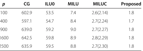
Table 1 Condition numbers for ap×pmatrix

p CG ILU0 MILU MILUC Proposed

100 602.9 53.5 7.4 2.6(2.14) 1.8

400 597.1 54.7 8.4 2.7(2.24) 1.7

900 639.0 59.2 9.0 2.7(2.27) 1.8

1600 642.5 59.8 8.9 2.8(2.29) 1.8

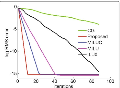
Figure 1Log RMS error curves for the2500×2500matrix of a simulation problem.

2.3 Convergence analysis

In this section, we analyze the convergence rate of the proposed preconditioner with the simulated data and real problems. We consider three measures for the evaluation of convergence rate, namely condition number, elapsed time and the amount of required memory. Specifically, the proposed method is compared with standard conjugate gradient without preconditioning, and several incomplete LU (ILU) factorization methods for the sparse symmetric system such as ILU0 [11], modified ILU (MILU) [11] and modified Crout variant of ILU (MILUC) [16].

First, we build a simulation problem for evaluating the convergence rate: we assume that an arbitrary image is the optimal solutionuo, and measure how fast the ui in

Algorithm 1 converges touo. Specifically, a linear system

(8) is built where the diagonal elementwi of the matrix

W is randomly generated within the range of [0 1], and

λis set to be 30. We need not specifically defined(x,y)

andg(x,y), because we need justbthat corresponds touo,

which is computed asb=(W−λL)uo. Given this linear

system, we compare the condition numbers in Table 1 for the matrices of moderate sizes ranging from 100×100 to 2500×2500. In this table, the density of nonzero elements of MILUC is given in the parenthesis, which is the ratio of the number of nonzero elements of MILUC to that of the

Table 2 Required memory space (KB), elapsed time (ms) and required iterations to reach the error of 10−3for a 250000×250000 matrix

CG ILU0 MILU MILUC Proposed

mem 32,6842 62,624 46,984 81,228 25,444

time 2.9661 0.8661 0.3201 872.56 0.2110

iters 62 20 7 4(2.33) 3

Table 3 Required memory space (KB), elapsed tie (ms) and number of required iterations to reach the error of 10−3 for the image sharpening example

CG ILU0 MILU MILUC Proposed

mem 16,396 24,770 36,652 43,128 13,272

time N/M 0.6596 0.1328 20.4474 0.1035

iters N/M 135 28 17(2.32) 10

original matrix. It can be seen that the proposed precon-ditioning method has the smallest condition number. The linear system with the lower condition number converges faster, which is also verified by plotting the log RMS error curve for the 2500×2500 case in Figure 1. The log RMS error is defined as log₁₀√|ui−uo|/N

, whereuidenotes

the solution after theith iteration, andNis the number of whole pixels.

We implement existing methods using MATLAB on a PC with Intel Core 2 quad (only a single core is used) and compare the number of iterations and CPU elapse time until the error reaches to 10−3, and also the amount of required memory. In this implementation, the size of the linear system is set to be 250000×250000. Note that all the steps in Algorithm 1, except for the step 4, are equally implemented for all the methods. The step 4 in our prob-lem is solved by using FFTW as stated previously. Table 2 shows the result that the amount of required memory space and CPU time for the proposed solver are less than those of others. It is found that the elapsed time of MILUC is much larger than others because it spends much time on the incomplete factorization of denser nonzero pattern. The ratio of the number of nonzero elements of MILUC to that of original matrix is also given in the parenthesis.

Second, the convergence rate is measured with two real problems: image sharpening and gradient domain

Table 4 Required memory space (KB), elapsed time(ms) and number of required iterations to reach the error of 10−3for the HDR imaging problem

Image size

CG ILU0 MILU MILUC Proposed

1025_× 769

mem 163,688 255,572 241,785 N/A 110,488

time N/M 53.9044 6.2435 N/A 5.5096

iters N/M 384 43 N/A 17

250× 150

mem 4,012 5,428 5,768 13,232 3,528

time N/M 0.4574 0.0936 11.3748 0.0516

iters N/M 148 26 15(2.32) 8

exposure fusion which will be addressed in the following section. The comparison for the image sharpening prob-lem is given in Table 3, which shows that the proposed method shows better performance than the others. In this table, there are N/M (not measured) in the case of CG because it hardly converges to the predefined log RMS error of (10−3) as observed in Figure 2. The comparison for the exposure fusion example is given in Table 4 where an additional experiment is conducted for the reduced image size (250×150), because MILUC causes an out-of-memory problem for the actual image size (1025×769). As shown in Table 4, the proposed method also shows bet-ter performance than the others. The convergence error curve for this problem is plotted in Figure 3.

3 Examples of weighted gradient domain image processing

In this section, we present two examples, image sharp-ening and gradient domain exposure fusion, where the gradient domain processing with the variable weights can be more effective than the existing approaches.

3.1 Image sharpening

Image sharpening is one of the most commonly used techniques for enhancing the contrast. The conventional

Figure 4Halo effect in conventional sharpening method.(a)

Input image.(b)Sharpened image by Laplacian subtraction [10].

method for image sharpening is the Laplacian subtraction approach, i.e., a Gaussian blur is applied to a given image, the blurred image is subtracted from the original to form a contrast image, and then the contrast image is weighted and added to the original. In this procedure, since the subtraction of blurred image from the original can be interpreted as an approximation of Laplacian filtering, this technique is called Laplacian substraction.

In the gradient domain processing, a similar operation to Laplacian subtraction has been developed in [10]. In this method, the energy function is designed based on (2), where d(x,y) is the input image and g(x,y) is designed such that the gradients are boosted as

g(x,y)= ∇d(x,y)(c1+c2s(x,y)), (12)

wherec1(>1)andc2are constants, ands(x,y)is a vector image containing the saliency in bothxandydirections around the pixel coordinate(x,y). According to the gra-dient manipulation strategy in (12), all the gragra-dients are basically boosted by constant valuec1and they are selec-tively magnified again by the edge saliency s(x,y). The parameterc2controls the amount of sharpening boosted bys(x,y). Although the gradient domain approach seems to be different from the Laplacian subtraction method, it has been shown that this approach can be interpreted as a generalized version of Laplacian subtraction method [10]. The images sharpened by the Laplacian subtraction sometimes suffer from halo effect which arises near object

Figure 5Image sharpening results.From the first to the third column are input image, results of conventional gradient domain method (Laplacian subtraction) in [10] and the proposed method.

boundaries. An example is shown in Figure 4b for the input image in Figure 4a. As can be seen in Figure 4b, there exists annoying halo around the edge although per-ceived contrast is enhanced to some extent. That is, there can be overshoot artifacts when stressing the contrast image too much. In order to reduce the halo effects we pose weights on the data term, which are given larger

values near the stronger edges and small values on tex-tureless areas, so that the pixel values on the less textured areas can be changed much while keeping the pixels val-ues around the strong edges. This weighting is formulated as

wi=(1−e−g

2

i/σd2_{), (13)}

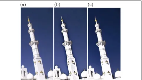
Figure 7Comparison of enhancement result.(a)Original.(b)Conventional method.(c)Proposed.

where gi is the gradient magnitude given by

d2_iv+d2_ih

withdivanddihbeing the vertical and horizontal gradient

value, respectively, andσ_dcontrols attenuation. Note that the gradient manipulation term in our solution is designed in the same manner as in (12).

The proposed sharpening is compared with the con-ventional gradient domain method in [10]. In Figure 5, the first column images are the inputs, the second shows the results of existing gradient domain method, and the last column shows the proposed. It can be observed that the previous method causes halo effect around the salient boundary, whereas the proposed method produces less

halo effect. Comparison on cropped area is also given in Figure 6, where the difference in the strong edges can be more easily observed. Results for another images are also shown in Figures 7 and 8, where bright or dark halo effects are also observed around the edges in the case of conventional enhancement result.

3.2 Weighted gradient domain exposure fusion

Dynamic range of natural scene is often much wider than that of commercial display and imaging sensors, and thus there have been many approaches to generating an HDR image from several differently exposed images. For

Figure 8Comparison of enhancement result for another image where dark halo is observed in the case of conventional method.

Figure 9Input images captured under different exposures.(a)Under-exposed image.(b)Over-exposed image.

displaying the HDR images so obtained on the LDR dis-plays, the tone-mapping is followed. More recently, the “exposure fusion” method has also been proposed, which generates a high quality image by the weighted summation of multi-exposure images [17]. When we do not have HDR displays, the exposure fusion is preferred because it skips the complicated process of expanding and compressing the dynamic ranges. In this method, using more images usually results in better quality. But a tripod is needed and there should be no moving object in the scene in order to prevent the ghost effects caused by hand trembling and moving objects. Hence the plausible HDR imaging with the hand held digital cameras is to use just two exposures:

an over-exposed image and an under-exposed one (see the images in Figure 9). However, using just two images sometimes brings loss of contrast.

For keeping all the contrasts perceived in two images, we design an energy function, where there are three func-tions to be considered:d(x,y),w(x,y), andg(x,y). First, the data functiond(x,y)is devised to keep the regions with better contrast in either of under or over exposed images, i.e.,

d(x,y)=

Iu(x,y), ifC(Iu(x,y)) >C(Io(x,y))

Io(x,y), otherwise

(14)

Figure 11Histogram of gradient magnitude.

whereIu(x,y)andIo(x,y)denote under- and over-exposed

image, respectively, andC(I(x,y))measures the contrast of the image I around pixel coordinate (x,y). However, such hard decision scheme in (14) would fail when the measured contrast is low. In other words, the reliability of the data function becomes low when the measured con-trast is low. We handle this problem by designing the data

weight functionw(x,y)in a spatially varying manner. To be specific,w(x,y)is designed such that the weight is close to one when the contrast is strong and to zero when the contrast is weak due to saturation, in the form of

w(x,y)=1−e−C(x,y)2/σ2, (15)

2 e r u s o p x E

(b)

e r u s o p x E

(a)

d e s o p o r P

(d)

o h t e m l a n o i t n e v n o C

(c)

(e)

(f)

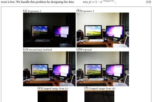
Figure 12Comparison for another set of multi-exposer images.(a)Exposure 1.(b)Exposure 2.(c)Conventional method.(d)Proposed.

whereC(x,y)=max{C(Iu(x,y),C(Io(x,y)}andσcontrols

the attenuation. The target gradient function g(x,y) is designed such that the larger gradient is preferred as

g(x,y)=

φ (∇Iu(x,y))∇Iu(x,y), if∇Iu(x,y) >∇Io(x,y)

φ (∇Io(x,y))∇Io(x,y), otherwise

(16)

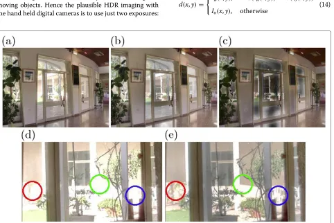
where φ (·) is a weight function which attenuates large gradients and magnifies small gradients, as defined in [1]. The result of our solution is compared with the intensity domain fusion [17] in Figure 10. Although the intensity domain exposure fusion method shows good performance in most of areas, it sometimes fails to preserve the con-trast as shown in Figure 10a (see outdoor areas). On the other hand, the proposed variable weight method pre-serves the contrast as shown in Figure 10b. The difference between the resulting images can be better perceived if we compare the cropped and magnified results as shown in Figure 10d,e, where the regions with noticeable differences are marked in the circles. For the objective compari-son, we compare the histogram of gradient magnitudes in the cropped region in Figure 11. It can be seen that the conventional exposure fusion has more zero gradi-ents (saturated pixels) than the proposed method. Also, the proposed method has more pixels around the gradi-ent magnitude of 0.1, which means that contrast is better preserved. To verify the effect of spatially varying weights, we also present a result with constant weight [10] in Figure 10c. Since the reliability of the data function is not considered in this case, the contrast is not well exposed and many regions remain dark, especially in textureless region. Another set of images for the comparison is shown in Figure 12, where it can be observed that the proposed method better keeps the contrast in dark regions such as the regions under the table and monitor. Figure 12e,f are the magnification of the regions under the table, which show the difference more clearly.

4 Conclusions

We have presented weighted gradient domain image pro-cessing problems where spatially varying weights are applied to the data term of conventional energy function. The problem is formulated as a system of linear equation, which is more efficiently solved by iterative methods such as PCG than by direct inverse or factorization methods. For solving the problem with the PCG, the most impor-tant thing is to find a preconditioning matrix that makes the system matrix have low condition number. We have shown that the system matrix for the constant weight problem is an appropriate choice for the preconditioner. Specifically, a subproblem in the PCG steps is efficiently solved by the proposed preconditioning matrix and it is

also shown that this matrix induces the convergent split-ting of the system matrix. Simulation and experiments also show that the proposed method converges faster than the existing methods, and also requires less memory space and CPU time. Applications of the weighted gra-dient domain image processing problems have also been presented, with the examples of image sharpening and the exposure fusion problems. In the comparison results, it is shown that better outputs are produced owing to the spatially varying design of data weight.

Competing interests

The authors declare that they have no competing interests.

Acknowledgements

This research was supported by Basic Science Research Program through the National Research Foundation of Korea (NRF) funded by the Ministry of Education, Science and Technology (2012-0000913).

Author details

1_{R&D team, Digital Imaging Business, Samsung Electronics, Gyeong-gi Do,}

Korea.2_{Department of Electrical and Computer Engineering and INMC, Seoul}

National University, Seoul, Korea.

Received: 7 June 2012 Accepted: 22 November 2012 Published: 23 January 2013

References

1. R Fattal, D Lischinski, W Michael, Gradient domain high dynamic range compression. ACM Trans. Graph.21(3), 249–256 (2002)

2. P P´erez, M Gangnet, A Blake, Poisson image editing. ACM Trans. Graph. 22(3), 313–318 (2003)

3. A Levin, A Zomet, S Peleg, Y Weiss, Seamless image stitching in the gradient domain. Lecture Notes Comput. Sci.3024, 377–389 (2004) 4. A Agarwala, Efficient gradient-domain compositing using quadtrees.

ACM Trans. Graph.26(3), 94–98 (2007)

5. J Jia, J Sun, CK Tang, HY Shum, Drag-and-drop Pasting. ACM Trans. Graph. 25(3), 631–637 (2006)

6. P Bhat, CL Zitnick, M Cohen, B Curless, GradientShop: a gradient-domain optimization framework for image and video filtering. ACM Trans. Graph. 29(2), 1–14 (2010)

7. S Baker, I Matthews, Lucas-Kanade 20 years on: a unifying framework. Int. J. Comput. Vis.56(3), 221–255 (2004)

8. Y Wu, J Fan, inCVPR’09. Contextual flow, (Miami, FL, 2009), pp. 33–40 9. J Sun, Z Xu, HY Shum, inCVPR’08. Image super-resolution using gradient

profile prior, (Anchorage, AK, 2008), pp. 1–8

10. P Bhat, B Curless, M Cohen, CL Zitnick, Fourier analysis of the 2D screened poisson equation for gradient domain problems. Lecture Notes Comput. Sci.5303, 114–128 (2008)

11. Y Saad,Iterative Methods for Sparse Linear Systems. (SIAM, Philadelphia, 2003)

12. TA Davis,Direct Methods for Sparse Linear Systems. (SIAM, Philadelphia, 2006)

13. M Benzi, Preconditionng techniques for large linear systems: a survey. J. Comput. Phys.182(2), 418–477 (2002)

14. FFTW. [http://www.fftw.org]

15. Intel Integrated Performance Premitive. [http://software.intel.com/en-us/ articles/intel-ipp/]

16. N Li, Y Saad, Y Chow, Crout versions of ILU for general sparse matrices. SIAM J. Sci. Comput.25(2), 716–728 (2003)

17. T Mertens, J Kautz, F Van Reeth, inPacific Graphics. Exposure fusion, (Maui, HI, 2007), pp. 382–390

doi:10.1186/1687-5281-2013-7