A Stochastic Version of the Jansen and Rit Neural Mass Model: Analysis and Numerics

DOI 10.1186/s13408-017-0046-4

R E S E A R C H Open Access

A Stochastic Version of the Jansen and Rit Neural Mass

Model: Analysis and Numerics

Markus Ableidinger1_{·Evelyn Buckwar}1_· Harald Hinterleitner1

Received: 26 September 2016 / Accepted: 23 May 2017 /

© The Author(s) 2017. This article is distributed under the terms of the Creative Commons Attribution 4.0 International License (http://creativecommons.org/licenses/by/4.0/), which permits unrestricted use, distribution, and reproduction in any medium, provided you give appropriate credit to the original author(s) and the source, provide a link to the Creative Commons license, and indicate if changes were made.

Abstract Neural mass models provide a useful framework for modelling mesoscopic

neural dynamics and in this article we consider the Jansen and Rit neural mass model (JR-NMM). We formulate a stochastic version of it which arises by incorporating ran-dom input and has the structure of a damped stochastic Hamiltonian system with non-linear displacement. We then investigate path properties and moment bounds of the model. Moreover, we study the asymptotic behaviour of the model and provide long-time stability results by establishing the geometric ergodicity of the system, which means that the system—independently of the initial values—always converges to an invariant measure. In the last part, we simulate the stochastic JR-NMM by an effi-cient numerical scheme based on a splitting approach which preserves the qualitative behaviour of the solution.

Keywords Jansen and Rit neural mass model·Stochastic Hamiltonian system· Asymptotic behaviour·Stochastic splitting schemes

1 Introduction

Neural mass models have been studied as models describing coarse grained activity of large populations of neurons [1–7] since the 1970s. They have successfully been used to fit neuroimaging data, understanding EEG rhythms [8] or epileptic brain dy-namics [9], and are now also a major building block in the Virtual Brain [10]. For a

B

[email protected]

M. Ableidinger

[email protected]

E. Buckwar

[email protected]

summary on their history, applications and an outlook on their future possible use, we refer to [11]. In general, neural mass models can be derived as a mean-field limit from microscopic models [12] and involve just a few state variables such as average membrane potentials and average population firing rates.

In this article, we focus on the Jansen and Rit neural mass model (JR-NMM) [13], which has been introduced as a model in the context of human electroencephalog-raphy (EEG) rhythms and visual evoked potentials [14]. It dates back to the work of Lopes da Silva and Van Rotterdam [3, 5, 15]. The JR-NMM is a biologically motivated convolution-based model of a neuronal population involving two subpop-ulations, i.e. excitatory and inhibitory interneurons forming feedback loops, which can describe background activity, alpha activity, sporadic and also rhythmic epileptic activity.

The original JR-NMM is formulated as a set of three coupled second-order non-linear ordinary differential equations (ODEs), i.e. these constitute a system of cou-pled nonlinear oscillators, often rewritten as the six-dimensional system of first-order equations. After introducing this system in Sect.2, we rewrite the system in the for-mat of classical mechanics, that is, as a damped Hamiltonian system with a nonlinear displacement. Furthermore, in most of the literature, the JR-NMM includes a term representing extrinsic input or background noise, which essentially is done by declar-ing that input function to be a stochastic process. Mathematically this implies that the solution process of the ODE system then also is a stochastic process inheriting the analytical properties of the input process and requiring some framework of stochas-tic analysis for its mathemastochas-tical treatment. In Sect. 3 we discuss options for such a framework and in this article we choose to formulate a stochastic JR-NMM as a stochastic differential equation (SDE) with additive noise, in particular a stochastic damped Hamiltonian system with a nonlinear term. Systems of SDEs of this or sim-ilar form are well studied in the molecular dynamics literature, where they are often called Langevin equations.1In this article we provide a range of results employing various techniques available in the framework of stochastic analysis developed for SDEs: In Sect.4we establish basic properties of the SDE such as moment bounds and bounds on the path behaviour. Section5augments existing analysis of the dy-namics of the deterministic JR-NMM, in particular we consider stochastic versions of equilibrium solutions, i.e. invariant measures, as well as the long-time behaviour of solutions of the SDE with respect to this invariant measure. These results may be interpreted as starting points for studies of phenomenological stochastic bifurcations or noise-induced transitions. Finally, in Sect.6, we present efficient numerical meth-ods designed for stochastic Hamiltonian problems and show that these numerical methods, which represent discrete stochastic systems for any fixed step-size, respect the properties previously established for the SDE system (subject to mild conditions on the step-size). Thus the resulting numerical methods will not only be quite effi-cient for future computational studies with the stochastic JR-NMM, they also provide

reliable computational results.

2 Description of the Original Jansen and Rit Neural Mass Model

A detailed summary of the model derivation from the neuroscientific point of view can be found in [18–20]. The main neural population, the excitatory and inhibitory interneurons, are in each case described by both a second-order ordinary differential operator, which transforms the mean incoming firing rate into the mean membrane potential, and a nonlinear function, which transforms the mean membrane potential into the mean output firing rate. Fort∈ [0, T]withT ∈R+, the JR-NMM proposed in [13] consists of three coupled nonlinear ODEs of second order

¨

x0(t )=AaSigm

x1(t )−x2(t )

−2ax˙0(t )−a2x0(t ), ¨

x1(t )=Aap(t )+C2SigmC1x0(t )−2ax1(t )˙ −a2x1(t ), (1)

¨

x2(t )=BbC4SigmC3x0(t )−2bx2(t )˙ −b2x2(t ),

which can be written as the six-dimensional first-order ODE system

˙

x0(t )=x3(t ),

˙

x1(t )=x4(t ),

˙

x2(t )=x5(t ),

˙

x3(t )=AaSigm

x1(t )−x2(t )

−2ax3(t )−a2x0(t ), ˙

x4(t )=Aap(t )+C2SigmC1x0(t )−2ax4(t )−a2x1(t ), ˙

x5(t )=BbC4SigmC3x0(t )−2bx5(t )−b2x2(t ),

(2)

with initial value(x0(0), . . . , x5(0))T =x0∈R6. Here, xi for i∈ {0,1,2}describe the mean postsynaptic potentials of distinct neuronal populations. The output

sig-nal y(t ):=x1(t )−x2(t ) describes the average membrane potential of the main

family, i.e. the principal neurons of the JR-NMM (see [18,19,21]). The function

p: [0, T] →Rdescribes the external input which may originate both from external sources or the activity of neighbouring neural populations. We will discuss the mathe-matical modelling ofpin more detail at the end of this section. The sigmoid function Sigm:R→ [0, νmax], νmax>0 (as suggested in [4]) is given by

Sigm(x):= νmax

1+er(v0−x)

and works as a gain function transforming the average membrane potential of a neural population into an average firing rate (see [22,23]). The constantνmaxdenotes the maximum firing rate of the neural population,v0∈Ris the value for which 50% of

the maximum firing rate is attained andr >0 determines the slope of the sigmoid function atv0.

Table 1 Typical values established in the original JR-NMM [13] taken from [19]

Parameter Description Typical value

A Average excitatory synaptic gain 3.25 mV

B Average inhibitory synaptic gain 22 mV

a−1 Time constant of excitatory postsynaptic potential 10 ms

b−1 Time constant of inhibitory postsynaptic potential 20 ms

C Average number of synapses between the populations 135

C1 Avg. no. of syn. established by principal neurons on excitatory interneurons C

C2 Avg. no. of syn. established by excitatory interneurons on principal neurons 0.8 C

C3 Avg. no. of syn. established by principal neurons on inhibitory interneurons 0.25 C

C4 Avg. no. of syn. established by inhibitory interneurons on principal neurons 0.25 C

νmax Maximum firing rate of the neural populations (max. of sigmoid fct.) 5 s−1

v0 Value for which 50% of the maximum firing rate is attained 6 mV

r Slope of the sigmoid function atv0 0.56 mV−1

a−1 andb−1 are corresponding time constants. The connectivity constantsCi for

i∈ {1,2,3,4}, modelling the interactions between the main population and interneu-rons, are assumed to be proportional to a single parameterCwhich characterises the average number of synapses between populations (see [13]). The solution behaviour of System (2) depends sensitively on the values of the parameters (we refer to the bi-furcation analyses in [18,19,24]). Especially, changes in the connectivity constants

Ci can result in drastic changes of the solution path.

Subsequently, we will employ the Hamiltonian formulation of classical mechanics to study coupled oscillators such as System (1) or (2). Let Q:=(x0, x1, x2)T and

P :=(x3, x4, x5)T denote three-dimensional vectors, then System (2) can be written as a damped Hamiltonian system with nonlinear displacement,

dQ

dt = ∇PH (Q, P ), dP

dt = −∇QH (Q, P )−2Γ P+G(t, Q).

(3)

In this formulation, the system consists of a Hamiltonian part with Hamiltonian func-tionH:R6→R+₀,

H (Q, P ):=1

2

P2_R3+ Γ Q

2 R3

,

a damping part with damping matrixΓ =diag[a, a, b] ∈R3×3, and a nonlinear part given by the functionG: [0, T] ×R3→R3, with

G(t, Q):=AaSigm(x1−x2), Aa

p(t )+C2Sigm(C1x0)

, BbC4Sigm(C3x0)

T

.

sum of the inductive and capacitive energy of the neuronal population, respectively. If the inputp(t )is a bounded deterministic function, the solution curve and the total energyH (Q, P )are bounded (this is an immediate result of Theorem4.2in Sect.4) and the time change in the total energy is given by

d

dtH (Q, P )= −2P

T_{Γ P+P}T_{G(t, Q).}

In the original paper by Jansen and Rit [13], the external input p(t ) has been used to represent spontaneous background noise as well as peak-like functions for generating evoked potentials. In the latter case the extrinsic input has been modelled as a deterministic periodic function (see also [25]) and with this type of input, the solution of the System (1) (or (2) or (3)) remains a deterministic function and the mathematical background to treat it is deterministic analysis. In the former case, i.e. whenp(t )represents spontaneous background noise and is modelled as a stochastic process, the mathematical background immediately changes to be stochastic analysis. In particular, the solution of the Systems (1), (2) or (3) becomes a stochastic process and it inherits the mathematical properties of the input processp(t ). Within stochastic analysis, (1), (2) or (3) may be interpreted in different frameworks, with consequences depending on the specific choices ofp(t ).

(i) Random Ordinary Differential Equation (RODE) framework: RODEs are path-wise ODEs involving a stochastic process in their right-hand side, i.e. for a suf-ficiently smooth functionf :Rm×Rd→Rd and anm-dimensional stochastic processξ(t ), ad-dimensional system of RODEs is given by

˙

x(t )=fξ(t ), x(t ),

(ii) Stochastic Differential Equation framework: If one were to choose the stochastic input process in an RODE as above as a Gaussian white noise process, one would need to deal with the fact that such a process exists only in the sense of

gener-alised stochastic processes; see [29], Sect. 3.2, or [30], Appendix I. In particular, Gaussian white noise is usually interpreted as the (generalised) derivative of the Wiener process, which itself is almost surely nowhere differentiable in the classi-cal sense. It is much more convenient to work in the classiclassi-cal stochastic analysis framework designed to deal with differential equations ‘subject to (white) noise’ and interpret Systems (1), (2) or (3) as a stochastic differential equation; see also [29], Sect. 4.1. A considerable amount of results concerning analysis, dynamics, numerics, statistics, etc. of SDEs is available and for stochastic numerics we refer for example to [31], which also treats SDEs driven by coloured noise.

3 Jansen and Rit Neural Mass Model as a Damped Stochastic

Hamiltonian System with Nonlinear Displacement

Let(Ω,F,P)be a complete probability space together with the filtration{Ft}t∈[0,T] which is right-continuous and complete. We extend the model of System (2) by al-lowing perturbation terms such asp(t )not only inx1(t )but in bothx0(t )andx2(t )as well. For this purpose, we define the functionsμi: [0, T] →Randσi: [0, T] →R+ for i∈ {3,4,5}. The functions μi will be used for representing deterministic in-put whereasσi will be used for scaling the stochastic components. In an analogous way to the exposition concerning stochastic oscillators in [32], Chap. 8, or in [33], Chap. 14.2, we symbolically introduce Gaussian white noise W˙i representing the stochastic input into Eq. (1) as follows:

dX0(t )=X3(t ) dt, dX1(t )=X4(t ) dt,

dX2(t )=X5(t ) dt,

dX3(t )=Aaμ3(t )+SigmX1(t )−X2(t )−2aX3(t )−a2X0(t )dt +σ3(t ) dW3(t ),

dX4(t )=

Aaμ4(t )+C2Sigm

C1X0(t )

−2aX4(t )−a2X1(t )

dt

+σ4(t ) dW4(t ),

dX5(t )=Bbμ5(t )+C4SigmC3X0(t )−2bX5(t )−b2X2(t )dt +σ5(t ) dW5(t ),

(4)

with deterministic initial value(X0(0), . . . , X5(0))T =X0∈R6. Here, the processes

we can use the(Q, P )-notation of classical mechanics

dQ(t )= ∇PH (Q, P ) dt,

dP (t )=−∇QH (Q, P )−2Γ P+G(t, Q)

dt+Σ (t ) dW (t ), (5)

with initial values

Q(0)=X0(0), X1(0), X2(0)T =Q0∈R3 and

P (0)=X3(0), X4(0), X5(0)

T

=P0∈R3,

diffusion matrix

Σ (t )=diagσ3(t ), σ4(t ), σ5(t )∈R3×3,

and nonlinear displacement

G(t, Q):=

⎛

⎝AaAa[[μ4(t )μ3(t )++SigmC2Sigm(X1(C1X0)−X2)]] Bb[μ5(t )+C4Sigm(C3X0)]

⎞ ⎠.

As before, we define the output signal asY (t )=X1(t )−X2(t ).

Systems of the type (5), typically called Langevin equations, have received con-siderable attention in the literature of molecular dynamics (see [16] for an overview). In particular, the long-time properties of such systems have been intensively studied in [34–36]. We employ these techniques in Sect.5to study the long-time behaviour of System (5).

We briefly discuss the existence of a solution of Eq. (5). As the sigmoid function Sigm is globally Lipschitz continuous, the existence and pathwise uniqueness of an

Ft-adapted solution is a standard result; see e.g. in [29], Theorem 6.2.2. In particular,

Qis continuously differentiable. In the current context, it makes sense to assume that the functionsμi andσi are smooth and bounded which we will do in the following.

We simulate the solution of Eq. (5) with the splitting integrator (24) proposed in Sect.6and illustrate the output signal in Fig. 1. The coefficients and the noise components are chosen in such a way that the simulation results of [14] for varying connectivity constantsCcan be reproduced. The numerical values for the parameters are given in Table1. For the deterministic part of the external inputs we setμ3=μ5=

0 andμ4=220, for the diffusion components we setσ3=σ5=10 andσ4=1,000

Fig. 1 Output signalY

4 Moment Bounds and Path Behaviour

We have already mentioned in Sect.2that the solution paths of Eq. (1) take values in a bounded set. It is natural to ask in which sense this behaviour transfers to the stochastic setting. We answer this question via a twofold strategy. On the one hand we will study the time evolution of the moments of the solution, which describes the average behaviour of all solution paths. On the other hand we will study the behaviour on the level of single paths and estimate the probability that a specific path exceeds a given threshold. Before we study these qualitative properties of Eq. (5) we provide a convolution-based representation for theQ-component of Eq. (5) which simplifies the corresponding calculations considerably.

4.1 Convolution-Based Representation of the JR-NMM

In this section we rewrite Eq. (5) usingX=(Q, P )T as

dX(t )=MX(t )+Nt, X(t )dt+S(t ) dW (t ), (6)

where

M=

O3 I3

−Γ2 −2Γ

,

Nt, X(t )=

03 G(t, Q(t ))

and

S(t )=

O3 Σ (t )

Fig. 2 Phase portraits

Here, we denote byO3,I3∈R3×3the zero and identity matrix, respectively.

More-over, we define 03:=(0,0,0)T and 13:=(1,1,1)T.

Note thatMis a block matrix with diagonal submatrices. Hence, we can calculate an explicit expression for the matrix exponential,

eMt =

e−Γ t_(I

3+Γ t ) e−Γ tt −Γ2e−Γ tt e−Γ t(I3−Γ t )

=:

ϑ (t ) κ(t ) ϑ(t ) κ(t )

. (7)

Theorem 4.1 The componentQof the unique solution of Eq. (5) solves fort∈ [0, T]

the integral equation

Q(t )=ϑ (t )Q0+κ(t )P0+

t

0

κ(t−s)Gs, Q(s)ds

+

t

0

κ(t−s)Σ (s) dW (s). (8)

We call Eq. (8) the convolution-based representation ofQin Eq. (5).

Proof Applying Itô’s formula ([29], Theorem 5.3.8) to the JR-NMM in Eq. (6) and using the commutativity ofMand eMt we obtain

de−MtX(t )=e−MtdX(t )−Me−MtX(t ) dt =e−MtNt, X(t )dt+S(t ) dW (t ),

which reads in integral form

X(t )=eMtX(0)+

t

0

eM(t−s)Ns, X(s)ds+

t

0

eM(t−s)S(s) dW (s).

Since the nonlinear part N only depends on Q the equation for Q is given by

Eq. (8).

Remark 1 From the latter proof we also get a convolution-based representation for

P, however, this formula depends onQ. Indeed, fort∈ [0, T],

P (t )=ϑ(t )Q0+κ(t )P0+

t

0

κ(t−s)Gs, Q(s)ds+

t

0

κ(t−s)Σ (s) dW (s).

Remark 2 System (1) has originally been deduced by using convolutions of impulse response functions with functions of the output from other subpopulations within the neural mass (see [13,18,37,38]). These response functions have the same shape as the kernelκin Eq. (8), which thus can be interpreted as the stochastic version of this kernel representation.

4.2 Moment Bounds

Using representation (8) we provide bounds on the first and second moment ofQ; analogous results can be derived forP. In the remainder of this section we will per-form various componentwise calculations and estimations. For ease and consistency of notation we define the following: Letx, y∈Rn, thenx≤y denotesxi≤yi for all 1≤i≤n. Furthermore, forU, V ∈Rn×k we denote the Hadamard product ofU

andV asUV, which is defined as the elementwise product (see [39,40]) such that each element of then×kmatrixUV is given as

In addition, we defineU2:=U U andU(1/2) as the elementwise root with

(U(1/2))ij=

Uij.

Theorem 4.2 Let μi : [0, T] →R+ for i ∈ {3,4,5} be nonnegative functions

bounded byμi,max∈R+, respectively, andCG:=(Aa(μ3,max+νmax), Aa(μ4,max+ C2νmax), Bb(μ5,max+C4νmax))T. ThenE[Q(t )]is bounded in each component by

ϑ (t )Q0+κ(t )P0≤E

Q(t )≤ϑ (t )Q0+κ(t )P0+Γ−2

I3−ϑ (t )

CG.

Proof We write

Q(t )=ϑ (t )Q0 +κ(t )P0

=:u(t )

+

t

0

κ(t−s)Gs, Q(s)ds

=:v(t )

+

t

0

κ(t−s)Σ (s) dW (s)

=:w(t )

.

Note that E[u(t )] =u(t ) and that the expectation of an Itô integral is zero, i.e.

E[w(t )] =06. Recall that Sigm:R→ [0, νmax], thus 03≤ G(t, Q(t ))≤ CG and also 03 ≤ E[G(t, Q(t ))] ≤ CG. Applying the latter bounds to E[v(t )] =

t

0κ(t−s)E[G(s, Q(s))]dsand integration ofκ yield the desired estimates.

Obviously, the bounds provided by Theorem4.2also hold for the deterministic equation (3) which justifies our claim in the introduction.

Remark 3 The upper bound depends linearly onμi,maxand the connectivity constants Ci whereasu(t )decays exponentially fast towards 03. In particular,

03≤ lim

t→∞E

Q(t )≤Γ−2CG.

Similar calculations can be done for the second moments of the components of

Q(t ). We obtain the following result.

Theorem 4.3 Let the assumptions of Theorem 4.2 hold and assume Σ (t ) to be a constant matrix, Σ ∈R3×3. We define for x =(x1, x2, x3)T ∈R3 the function

1+(x):=(1+(x1),1+(x2),1+(x3))T, where 1+denotes the indicator function of the

setR+. Using the functionsu,v and wfrom Theorem4.2, a bound for the second

moment of each component ofQ(t )reads

EQ2(t )

≤u2(t )+2u(t )1+u(t )Γ−2I3−ϑ (t )

CG

+

Γ−2I3−ϑ (t )

CG+ 1 2Γ

−3/2_ΣI

3+κ(t )ϑ(t )−ϑ2(t )

1/2

13

2 .

In particular,

lim t→∞E

Q2(t )≤

Γ−2CG+ 1 2Γ

−3/2_Σ

13

Fig. 3 Time evolution ofE[X1]

Proof From the proof of Theorem4.2it immediately follows that

Eu2(t )=u2(t ), Ev2(t )≤Γ−4I3−ϑ (t )

2

C_G2 and (9a)

Ew2(t )=1

4Γ

−3_Σ2_I

3+κ(t )ϑ(t )−ϑ2(t )

13. (9b)

The last equality can be shown by applying the Itô isometry. For notational simplic-ity we omit the dependence ont in the following. By using the Cauchy–Schwarz inequality we bound

E[vw] ≤Ev2Ew2(1/2).

Applying the bounds (9a)-(9b), the desired result follows from

EQ2 = u2+Ev2+Ew2+2uE[v] +2E[vw] ≤u2+2u1+(u)E[v]

+Ev2(1/2)+Ew2(1/2)2.

In Fig.3we employ Monte Carlo simulation to estimateE[X1(t )]for varying cou-pling parameterC. The results for the second momentE[X2₁(t )]are essentially the same; see Fig.4. Similar results can be obtained forX2andX3. The numerical

Fig. 4 Time evolution ofE[X2₁]

(red curves), whereas single trajectories (purple curves) of course may exceed the bounds of the average. Note that, forC=68,135 and 675, the approximations of

E[X1(t )]rapidly converge towards fixed values for growingt. The same behaviour can be observed forC=270 on larger time scales. We will give a theoretical ex-planation for this phenomenon in Sect.5when we study the long-time behaviour of Eq. (5).

4.3 Pathwise Bounds

Theorem4.2states that on average the solution of Eq. (5) stays in some bounded set. However, the theorem gives no information for single solution paths, which can in principle attain arbitrarily large values with positive probability; see LemmaA.2 in theAppendix. In this section we want to quantify the probability of such large values. The following theorem provides an upper bound on the escape probability of the components ofQ, i.e. the probability that fori∈ {0,1,2}the solutionXi is larger than a given thresholdx_it h∈R+.

Theorem 4.4 Let the assumptions of Theorem4.3hold. For fixedt∈ [0, T]we define a Gaussian random vectorY (t )=(Y0(t ), Y1(t ), Y2(t ))with

EY (t )=u(t )+Γ−2I3−ϑ (t )

CG and

CovY (t )=1

4Γ

−3_Σ2_I

3+κ(t )ϑ(t )−ϑ2(t )

,

where its componentsYi(t )are independent. LetFYi(t ) denote the cumulative

dis-tribution function of Yi(t ). Then the probability that the components Xi(t ) for

i∈ {0,1,2}exceed the given thresholdsx_it h∈R+is bounded by

PXi(t )≥x_it h

≤1−FYi(t )

Fig. 5 Pathwise bounds ofX1

Proof From Eq. (8), the bound onGand again integratingκ, we immediately see that each path ofQis bounded by the stochastic processY defined by

Y (t )=u(t )+Γ−2I3−ϑ (t )

CG+ t

0

κ(t−s)Σ dW (s).

The processY (t )is Gaussian distributed with meanu(t )+Γ−2(I3−ϑ (t ))CGand covariance matrix 1₄Γ−3Σ2(I3+κ(t )ϑ(t )−ϑ2(t )), which were calculated in

The-orems4.2and4.3. Then, for eacht∈ [0, T],

PXi(t )≥xit h

≤PYi(t )≥xit h

=1−FYi(t )

x_it h.

Remark 4 Theorem4.4can, for example, be used for calibration of the noise pa-rameters inΣ. LetΣ=diag[σ3, σ4, σ5]. Suppose we want to chooseσ3 such that the corresponding componentX0(t )stays below some given thresholdx₀t hwith high

probabilityα. Then a suitable choice ofσ3is implicitly given byFY0(t )(x t h

0 )=α.

In Fig. 5 we illustrate numerical trajectories of Eq. (5) and the corresponding bounds for varying levels ofα, i.e. for a given time pointt, the probability ofX1(t )to be below the red, purple and black curve is at least 60, 90 and 99 percent, respectively.

5 Long-Time Behaviour and Stationary Solutions

equation (3) can possess several equilibrium solutions (both stable and unstable) as well as limit cycles with typically nontrivial basins of attraction (again we refer to the bifurcation analyses in [18,19,24]). Thus, the choice of the initial value can have large impact on the long-time behaviour of the solution curves of Eq. (3). From a practical point of view, this fact may be problematic, as it is not at all obvious how to estimate the initial value of theP-component.

In this section, we will analyse a stochastic counterpart of equilibrium solutions, more precisely invariant measures, and study the long-time asymptotics of Eq. (5). Our main tool is the theory of ergodic Markov processes, for convenience of the reader we recapitulate the basic definitions.

Let(X(t ))t∈[0,T]be the solution process of Eq. (5). Standard stochastic analysis shows thatX(t ) is a Markov process and the corresponding transition probability

Pt(A, x), i.e. the probability thatX(t )reaches a Borel-setA⊂R6at timet, when it started in the pointx∈R6at timet=0, is given by

Pt(A, x):=P

X(t )∈A|X(0)=x.

We use the definition provided in [41], Chap. 2, to characterise invariant measures. For simplicity, letηbe a probability measure on(R6,B(R6))(in generalηcan de-generate on some lower dimensional space). The measureηis called invariant if

η(A)=

R6Pt

(A, x)η(dx) ∀A∈BR6,∀t∈ [0, T].

In particular, if we set the initial value(Q0, P0)to be a random vector with distri-butionη, then there exists a Markov process X(t )which satisfies Eq. (5) and the distribution of X(t )is η for all t ∈ [0, T]. In this sense, the concept of invariant measures can be seen as a natural extension of stationary solutions of deterministic ODEs.

We are interested in the following questions: (i) Does Eq. (5) have an invariant measure? (ii) Is the invariant measure unique?

(iii) Do quantities of the typeE[h(X(t ))]converge towards stationary values for a suitable class of functionsh:R6→Rand any initial value(Q0, P0)?

We answer these questions in two steps: In the first step we will show that Eq. (5) fulfills a Lyapunov condition ensuring the existence of (possibly many) invariant measures. The questions (ii) and (iii) will be answered positively via the concept of geometric ergodicity. In classical mechanics and molecular dynamics, equations with a similar structure as Eq. (5), termed Langevin equations in the corresponding literature (see e.g. [16,31,36]), are well studied and we make use of relevant results concerning the long-time behaviour. In particular, we follow the presentation in [34]. As in the bifurcation analyses for Eq. (3) mentioned before, we assume that the deterministic parts of the perturbation as well as the diffusion matrix are constant, i.e.

5.1 Existence of Invariant Measures and Geometric Ergodicity

The existence of invariant measures for Eq. (5) can be established by finding a suit-able Lyapunov function. Heuristically speaking, the existence of a Lyapunov func-tion ensures both that the solufunc-tion trajectories stay in some bounded domain (except for some rare excursions) and in the case of excursions, the trajectories return to the bounded set. The following lemma shows that a perturbed version of the Hamiltonian

Hin Eq. (5) can act as a Lyapunov function (see [42]).

Lemma 5.1 Assumea, b >0 and let forn∈N

Vn(Q, P ):=

1+1 2P

2 R3+

3 2Γ Q

2

R3+ P , Γ Q n

, n∈N.

ThenVnis a Lyapunov function for Eq. (5) in the following sense:

(i) Vn≥1 andVn→ ∞for(Q, P )T_R6→ ∞, (ii) ∃αn<0,βn>0 such that

LVn≤αnVn+βn,

whereLdenotes the generator of Eq. (5),

L:=PT∇Q+

−QTΓ2−2PTΓ +G(Q)T∇P + 1 2

5

i=3 σ_i2 ∂

2 ∂X_i2.

Here,∇Qand∇P denote the gradient with respect to theQandP component,

respectively.

Proof For a, b >0, Property (i) is satisfied by construction and we only have to prove (ii). In a first step we setn=1 and analyse the action ofLonV1. Note thatV1is quadratic, therefore the second derivatives inLresult in constants. SincePTΓ2Q= QTΓ2P, we obtain

LV1=PT

3Γ2Q+Γ P

+−QTΓ2−2PTΓ +G(Q)T(P+Γ Q)+1

2

5

i=3 σ_i2

= −PTΓ P−QTΓ3Q+1

2

5

i=3

σ_i2+G(Q)T(P+Γ Q). (11)

The first two terms in Eq. (11) are quadratic and non-positive. AsV1is quadratic and non-negative, there always exist constantsα <0 andβ >0 such that the first three terms in Eq. (11) can be bounded in the following way:

−PTΓ P−QTΓ3Q+1

2

5

i=3

Furthermore, Young’s inequality implies

G(Q)T(P+Γ Q)≤

2

P2_R3+ Γ Q

2 R3

+ 1

2G(Q) 2 R3,

where >0 can be chosen arbitrarily small. Thus, there existα < α <0 andβ >0 sufficiently large such that

LV1(Q, P )≤αV1(Q, P )+β. (12) In a second step, we will extend this procedure toVnforn∈N. For brevity we use the notation

L2:=1

2

5

i=3 σ_i2 ∂

2

∂X2_i and L1:=L−L2.

L1is a first-order differential operator and the action ofL1onVncan be bounded in the following way by using Eq. (12):

L1Vn=nVn−1L1V1≤αnVn+nβVn−1.

ApplyingL2toVnleads to

L2Vn=

n

2

5

i=3 σ_i2

Vn−1 ∂2V1

∂X_i2 +(n−1)Vn−2

∂V1 ∂Xi

2

=n

2

5

i=3

σ_i2Vn−1+(n−1)Vn−2(Xi+Γi−2,i−2Xi−3)2

,

whereΓi,j denotes the entry ofΓ at the intersection of theith row andjth column. Note that

5

i=3

σ_i2(Xi+Γi−2,i−2Xi−3)2≤max

σ₃2, σ₄2, σ₅2Γ Q+P2_R3.

This implies that there existc, cn>0 such that

n(n−1)

2 Vn−2

5

i=3

σ_i2(Xi+Γi−2,i−2Xi−3)2≤cVn−1,

and thus

L2Vn≤cnVn−1.

As a consequence, there existαn<0 (possibly close to zero) andβn>0 such that

LVn=L1Vn+L2Vn≤αnVn+(nβ+cn)Vn−1≤αnVn+βn,

Lemma5.1has two immediate consequences. First, applying Itô’s formula onVn we obtain the following bounds (see [34]).

Corollary 5.2 Let Assumption (10) hold ands, t∈ [0, T]witht≥s. Then

EVn

Q(t ), P (t )|F(s)≤e−|αn|(t−s)Vn

Q(s), P (s)+ βn |αn|

1−e−|αn|(t−s).

In particular,

EVn

Q(t ), P (t )≤e−|αn|t_V n

Q(0), P (0)+ βn |αn|

1−e−|αn|t_.

Second, the existence of a Lyapunov function ensures the existence of an invariant measure (see e.g. [43], Corollary 1.11).

Corollary 5.3 Let Assumption (10) hold and letX(t )denote the solution of Eq. (5).

Then there exists an invariant measureηofX(t ).

Lemma5.1does not give any information on the uniqueness of the invariant mea-sure. If we further assume that the three Wiener processesWi act on all components ofP, i.e.σi>0 fori∈ {3,4,5}, we can establish the uniqueness of the invariant mea-sure. Furthermore, the Markov processXfulfills the property of geometric ergodicity in the sense of [34]. We give a modification of the result in [34], Theorem 3.2, in-cluding the nonlinear functionG.

Theorem 5.4 Letσi >0 for alli∈ {3,4,5}. The Markov process X(t )defined by

Eq. (5) has a unique invariant measureηonR6. Furthermore, let

Hn:=

h:R6→RBorel-measurable with|h| ≤Vn

.

Then for anyn∈Nand any initial valueX(0)=(Q0, P0)there exist positive

con-stantsCn,λnsuch that

EhX(t )−

R6

h dη≤CnVn

X(0)e−λnt ∀h∈Hn,∀t≥0.

Proof The proof is the same as in [34]. The Lyapunov condition has been estab-lished in Lemma5.1, the corresponding results for the necessary smoothness of the transition probabilities and the irreducibility of the Markov process are given in the Appendixin LemmaA.2andA.1. Both lemmas rely on the assumption thatσi>0

fori∈ {3,4,5}.

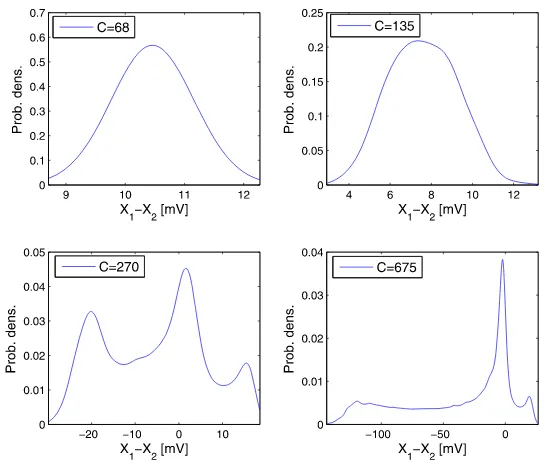
Fig. 6 Densities of the invariant measure ofY

Second, due to the correspondence of the time averages and “space averages” of er-godic systems (see [41], Theorem 3.2.4.), one can estimate quantities of the type

E[h(X(t ))](fort sufficiently large) by computing the time average of a single path ofX(t )on a large time horizon instead of using Monte Carlo estimation which re-quires one to compute a large number of paths ofX(t ). Of course, both aspects hold only true if the numerical method reproduces the geometric ergodicity of the original system (see Sect.6).

6 Numerical Simulation

In order to obtain an approximation of Eq. (5) which accurately reproduces the qual-itative behaviour, it is highly important to construct numerical integrators which on the one hand fulfil the properties of Eq. (5) derived in Sects.4and5, and on the other hand are computationally efficient such that large ensembles of trajectories can be calculated in reasonable time.

We want to emphasise that the difficulty does not lie in the construction of a mean-square convergent integrator for Eq. (5). In fact, as the coefficient functions of Eq. (5) are globally Lipschitz continuous, any standard integrator (e.g. the Euler–Maruyama method) converges in the mean-square sense. However, it has already been shown for linear stochastic oscillators that the Euler–Maruyama method does not preserve second moment properties of that system [48] and it is expected that this negative result extends to nonlinear stochastic oscillators as well. The splitting methods fulfil the following properties:

(i) The methods preserve the moment bounds proposed in Theorems4.2and4.3. Furthermore, for Σ=O3, the numerical method preserves the bounds of the

exact solution.

(ii) The Markov process generated by the numerical method is geometrically ergodic and fulfils a Lyapunov condition under very mild step-size restric-tions.

6.1 Splitting Integrators for the JR-NMM

For convenience of the reader we provide a brief introduction to splitting integra-tors. Further details can be found, for example, in the classical monograph [49], Chapter II, for the deterministic case and [35,50] for stochastic Langevin-type equa-tions.

The main idea of splitting integrators is the following: Assume for simplicity we want to approximate a deterministic ODE system

˙

y=f (y), y(0)=y0∈Rn

for which the functionf:Rn→Rncan be written as

f (y)=

d

i=1

f[j](y), wheref[j]:Rn→Rnforj∈ {1, . . . , d}.

Of course, there can be several possibilities to decomposef. The goal is to choose

f[j]in such a way that the subsystems

˙

y=f[j](y), j ∈ {1, . . . , d}, (13)

can be solved exactly. Letϕ_t[j](y0)denote the exact flow of the Subsystem (13) with

deter-ministic order one (Lie–Trotter splitting) and two (Strang splitting):

Ψ_tLT(y)=ϕ_t[1]◦ · · · ◦ϕ[_td](y),

Ψ_tS(y)=ϕ_{t /}[1]₂◦ · · · ◦ϕ_{t /}[d−₂1]◦ϕ[_td]◦ϕ_{t /}[d−₂1]◦ · · · ◦ϕ[_{t /}1]₂(y).

This strategy can be extended to the stochastic setting (see [35] and the references therein for splitting integrators in the field of molecular dynamics, [50] for quasi-symplectic splitting integrators, [51] for variational integrators based on a splitting approach and [52] for splitting integrators in a Lie group setting). In particular, split-ting integrators have been applied efficiently to Langevin equations with a similar structure as Eq. (5), see [35,50], thus we extend this approach here to Eq. (5).

The main step in the construction of splitting integrators is to choose a suitable decomposition of the coefficient functions of Eq. (5). The right-hand side decom-poses into three rather distinct parts: First, a damped, linear oscillatory part, second, a nonlinear and non-autonomous coupling part which does not depend on the P -component, and third, a stochastic part which does only arise in theP-component. Therefore, dQ dP =

∇PH (Q, P )

−∇QH (Q, P )−2Γ P

damp. lin. oscill.

dt+ 03 G(t, Q) nonlin. coupl. dt+ 03 Σ (t ) dW (t )

stochastic

with the nonlinear term given by

G(t, Q)=GI(t )+GII(Q):=

⎛

⎝Aaμ3(t )Aaμ4(t ) Bbμ5(t )

⎞ ⎠₊

⎛

⎝AaAaC2SigmSigm(X1(C1X0)−X2) BbC4Sigm(C3X0)

⎞ ⎠.

It makes sense to split the linear and the nonlinear drift contributions, thus providing two options to incorporate the stochastic noise. This yields two different sets of sub-systems and therefore two different sets of numerical methods. In the first case, the stochastic subsystem defines a general Ornstein–Uhlenbeck process and we denote the corresponding splitting integrator as Ornstein–Uhlenbeck integrator. In the sec-ond case, the stochastic subsystem defines a Wiener process with drift and we denote the splitting integrator as Wiener integrator.

In the following let 0=t0<· · ·< tN=T withN∈Nbe an equidistant partition of[0, T]with step-sizet.

6.2 Ornstein–Uhlenbeck Integrator

The first variant is to include the stochastic contribution into the linear oscillator part, which gives rise to the two following subsystems:

dQ[1] dP[1]

=

∇P[1]H (Q[1], P[1]) −∇Q[1]H (Q[1], P[1])−2Γ P[1]

dt+

03 Σ (t ) dW (t )

, (14a)

dQ[2] dP[2]

=

03 G(t, Q[2])

For both subsystems we can easily derive explicit representations of the exact solu-tions which can be used directly for the numerical simulation. Subsystem (14a) is a six-dimensional Ornstein–Uhlenbeck process. LetX[1](ti)=(Q[1](ti), P[1](ti))T denote the solution of Eq. (14a) at time pointti fori∈ {0, . . . , N−1}, then the exact solution at time pointti+1> ti can be represented as

X[1](ti+1)=eMtX[1](ti)+ ti+1

ti

κ(ti+1−s)Σ (s) dW (s) κ(ti+1−s)Σ (s) dW (s)

, (15)

whereeMt is defined in Eq. (7).X[1]is a Gaussian process with conditional expec-tation

EX[1](ti+1)|Fti

=eMtX[1](ti) and the conditional covariance matrix (see [29], Theorem 8.2.6)

Cov(ti+1):=Cov

X[1](ti+1), X[1](ti+1)|Fti

=EX[1](ti+1)−E

X[1](ti+1)

X[1](ti+1)−E

X[1](ti+1) T

|Fti

=

ti+1

ti

eM(ti+1−s)_Σ2_(s)eM(ti+1−s)T_ds.

In particular, the integral term in Eq. (15) can be simulated exactly. Indeed, it is Gaussian distributed with mean zero and covariance matrix Cov(ti+1), which is for

t≥ti given as the unique solution of the matrix-valued ODE

dCov(t )

dt =MCov(t )+Cov(t )M

T ₊

O3 O3

O3 Σ2(t )

, (16)

Cov(ti)=O6.

In the special case of a constant diffusion matrixΣ (t )=Σ∈R3×3, the exact solution of Eq. (16) can be explicitly calculated fort≥0 as

Cov(ti+t )

=

₁

4Γ−3Σ2(I3+κ(t )ϑ(t )−ϑ2(t ))

1

2Σ2κ2(t ) 1

2Σ

2_κ2_{(t )} 1

4Γ− 1_Σ2_(I

3+κ(t )ϑ(t )−κ2(t ))

.

In general, Eq. (16) has to be solved by numerical approximation, however, it only needs to be precomputed once for the step-sizet. In either case, we obtain

X[1](ti+1)=eMtX[1](ti)+ξi(t ), (17) where ξi(t ) are iid six-dimensional Gaussian random vectors with expectation

E[ξi(t )] =06and covariance matrix Cov(t ).

the solution of Eq. (14b) at time pointti, then the exact solution at time pointti+1> ti is given by

Q[2](ti+1)=Q[2](ti),

P[2](ti+1)=P[2](ti)+ ti+1

ti

Gs, Q[2](s)ds (18)

=P[2](ti)+t GII

Q[2](ti)

+

ti₊1

ti

GI(s) ds,

where we assume that the last integral can be calculated exactly.

Now, letϕ_tou,[1]andϕ_tou,[2]denote the exact flows of Eq. (14a) and (14b) given via Eq. (17) and (18), respectively. Letx∈R6, then a one-step integrator is defined by the composition of the flows

ψ_tou(x)=ϕ_tou,[1]◦ϕ_tou,[2](x). (19)

6.3 Wiener Integrator

The second possibility is to include the stochastic terms into the nonlinear contribu-tion yielding the subsystems

dQ[1] dP[1]

=

∇P[1]H (Q[1], P[1])

−∇Q[1]H (Q[1], P[1])−2Γ P[1]

dt, (20a)

dQ[2] dP[2]

=

0

G(t, Q[2])

dt+

0

Σ (t ) dW (t )

. (20b)

Subsystem (20a) is a deterministic system. LetX[1](ti)=(Q[1](ti), P[1](ti))T denote the solution of Eq. (20a) at time pointti, then the exact solution at time pointti+1is

given by

X[1](ti+1)=eMtX[1](ti). (21) The solution of subsystem (20b) is—by definition—given by

Q[2](ti+1)=Q[2](ti),

P[2](ti+1)=P[2](ti)+t GII

Q[2](ti)

(22)

+

ti₊1

ti

GI(s) ds+

ti₊1

ti

Σ (s) dW (s),

where the last term can be simulated exactly as a three-dimensional Gaussian random vector with zero mean and covariance matrixti+1

ti Σ

2_{(s) ds. In the case of a constant}

one-step integrator for Eq. (5) is given by

ψ_tw(x)=ϕ_tw,[1]◦ϕ_tw,[2](x). (23)

6.4 Order of Convergence and Strang Splitting

As the noise in Eq. (5) is additive, standard integrators such as the Euler–Maruyama method converge with mean-square order one. The same holds true for the splitting integrators constructed above.

Theorem 6.1 Let 0=t0<· · ·< tN=T be an equidistant partition of[0, T]with

step-sizet, and letXou(ti)andXw(ti)denote the numerical solutions defined by

Eq. (19) and (23) at time pointti starting at initial value(Q0, P0)∈R6. Then the

one-step methods defined in Eq. (19) and (23) are of mean-square order one, i.e.

there exist constantsC1, C2>0 such that for sufficiently smalltthe inequalities

EX(ti)−Xou(ti)

2 R6

1/2

≤C1t,

EX(ti)−Xw(ti)

2 R6

1/2

≤C2t,

hold for all time pointsti.

Proof The result can be proved in the same way as in [50], Lemma 2.1..

For deterministic ODE systems the convergence order of splitting methods can be increased by using composition based on fractional steps (see e.g. [49], Chapter II). We will illustrate this approach for the method based on the subsystems (20a) and (20b), the other method can be treated analogously. Using a Strang splitting we can compose the integrator

ψ_tw(x)=ϕ_{t /}w,[1₂]◦ϕ_tw,[2]◦ϕ_{t /}w,[1₂](x), x∈R6. (24) ForΣ=O3, Eq. (24) is a second-order method for the deterministic Eq. (2), however,

the mean-square order of Eq. (24) is still one. To increase the mean-square order one has to include higher-order stochastic integrals to reproduce the interactions of the Subsystems (20a) and (20b) (see [50], Sect. 2, for details). Note that even without including the higher-order stochastic integrals the Strang splitting integrator given by Eq. (24) performs considerably better in our numerical simulations than the Lie– Trotter methods, thus we recommend to use this type of integrator. We have not yet studied the reason for this improved performance, but expect that the symmetry of the Strang splitting or the weak noise acting on the system may contribute.

Fig. 7 Mean-square convergence of the splitting method

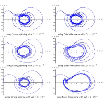
Fig. 8 Phase portrait of one single path ofY

or when the Euler–Maruyama method is embedded in a continuous-time particle fil-ter.

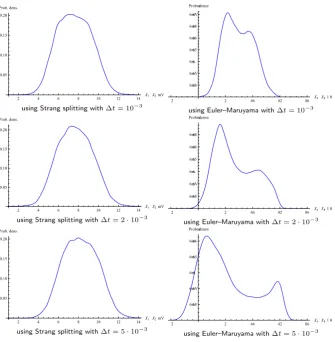
Fig. 9 Densities of the invariant measure ofY

step-sizes than those required for the Euler–Maruyama method. The other important feature of the proposed method is its reliability. Figure8shows several plots of the phase portrait of one single path of the outputY, with the splitting method and the Euler–Maruyama method and different step-sizes. It can be observed that the phase portrait obtained with the latter method changes markedly with increasing step-size. These phase portraits have been computed for the coupling parameterC=135, initial valueX(0)=06,σ3=σ5=1,σ4=200 andt∈ {10−4,10−3,2·10−3}. Figure9

corresponds to the upper right plot in Fig.6, which itself can be interpreted as a computational study of a phenomenological stochastic bifurcation for varying cou-pling parameterC. It shows the densities of the invariant measure ofY forC=135,

σ3=σ5=10 andσ4=103and compares the Strang splitting scheme with the Euler–

6.5 Moment Bounds and Geometric Ergodicity

The following two lemmas represent the properties presented in Sect.4for the numer-ical approximation schemes defined by Eq. (19) and Eq. (23). LetXou=(Qou, Pou)

andXw=(Qw, Pw)denote the numerical solutions defined by Eq. (19) and Eq. (23), respectively. We start with proving analogous bounds to those in Theorem4.2for the expected value of Qou andQw. It is well known already in the deterministic set-ting that the Euler scheme does not preserve such properties, see [49], Chap. 1, in the stochastic case negative results for the Euler–Maruyama method for (simple) stochas-tic oscillators have been observed in [48]. Note that the following two lemmas also hold when commuting the compositions in Eq. (19) and Eq. (23).

Lemma 6.2 Let μj : [0, T] →R+ for j ∈ {3,4,5} be non-negative functions

bounded byμj,max∈R+, respectively. Then fori∈ {0, . . . , N},E[Qw(ti)](and also

E[Qou(ti)]) is bounded in each component by

ϑ (ti)Q0+κ(ti)P0≤E

Qw(ti)

≤ϑ (ti)Q0+κ(ti)P0+Γ−2CG.

Proof We prove the result for the numerical methodψw,ψou can be treated analo-gously. Bearing in mind the notation in Sect.4, we obtain from Eq. (23) that

EXw(ti)

=eMtEXw(ti−1)

+eMtENti−1, Xw(ti−1)

t

=eMti_X(0)+ i

k=1

eMtkE_Nt

i−k, Xw(ti−k)

t,

and in particular itsQ-component reads

EQw(ti)

=ϑ (ti)Q0+κ(ti)P0+ i

k=1 κ(tk)E

Gti−k, Xw(ti−k)

t. (25)

From the proof of Theorem4.2we obtain 03≤E[G(ti−k, Xw(ti−k))] ≤CG. Obviously, the lower bound ofE[Qw(ti)]is fulfilled for any time step-sizet. To prove the upper bound it remains to show that

i

k=1

κ(tk)t≤Γ−2.

From the decomposition

i

k=1

κ(tk)t=

I3−e−Γ t

₋1

I3−e−Γ ti

κ(t )t−κ(t )κ(ti)

+e−Γ t

i

we derive the formula

i

k=1

κ(tk)t=

I3−e−Γ t

₋2

I3−e−Γ ti

κ(t )t

−I3−e−Γ t

₋1

κ(t )κ(ti),

which is in each component smaller thanΓ−2for any time step-sizet.

Remark 5 Another viewpoint of Eq. (23) is to apply the rectangle method (using the left boundary point of the integral) in order to approximate the convolution-based formula Eq. (8) in the form

Q(t+t )=ϑ (t )Q(t )+κ(t )P (t )

+

t+t

t

κ(t+t−s)Gs, Q(s)ds

+

t+t

t

κ(t+t−s)Σ (s) dW (s).

Moreover, Eq. (25) permits better insight into the distinction of the numerical schemes: The sum in Eq. (25) corresponds to the rectangle method in order to approx-imate the convolution integralE[v(t )]defined in the proof of Theorem4.2, where the right boundary point is used in each approximation interval. Analogously, when com-muting the composition in Eq. (23) one obtains the rectangle method evaluating the left boundary points. In the case of the Strang splitting scheme given by Eq. (24), the functionκ is evaluated at the midpoints(tk+tk+1)/2.

Remark 6 It can be shown analogously that the second momentE[(Qw(ti))2](and alsoE[(Qou(ti))2]) is bounded by

EQw(ti) 2

≤u2(ti)+2u(ti)1+

u(ti)

Γ−2CG

+

Γ−2CG+ 1 2Γ

−3/2_Σ1 3

2 .

Lemma 6.3 Let 0< t0· · ·< tN =T be an equidistant partition of [0, T] with

step-sizet <1/(2ΓL∞)and letXw denote the numerical solutions defined by

Eq. (23). Then the functionalV (X):=V1(Q, P )defined in Lemma5.1is a Lyapunov function forXw, i.e. there exist constantsα∈(0,1)andβ≥0 such that

EVXw(ti+1)

|Fti

≤αVXw(ti)

+β.

Proof For the sake of simplicity we seta=b, which implies e−Γ tx =e−atx for anyx∈R3. Furthermore, we denoteQ:=Q(ti), P :=P (ti)to shorten notation. The one-step approximationsQ(ti+1)andP (ti+1)can be written as

Γ Q(ti+1)=Γ e−at(I3+Γ t )Q+Γ e−att

P +t G(Q)+Σ ξ,

P (ti+1)=e−at(Γ Q+P )+e−att G(Q)+e−atΣ ξ−Γ Q(ti+1), whereξ ∼N(03,I3)is a three-dimensional Gaussian vector independent ofFti. By elementary calculations and application of Young’s inequality we obtain

1

2P (ti+1)+Γ Q(ti+1)

2 R3

≤ 1

2e

−2at_{Γ Q+P}2

R3+

2e

−4at_t2_{Γ Q+P}2

R3

+ 1

2G(Q) 2 R3+

1 2e

−at_{t G(Q)+Σ ξ}2

R3

+e−2atΓ Q+P , Σ ξ_R3,

where >0 is a parameter which can be freely chosen. Thus, one can findC1>0

sufficiently large such that

1

2EP (ti+1)+Γ Q(ti+1)

2 R3|Fti

≤1

2e

−2at_{Γ Q+P}2

R3+ 1

2G(Q) 2 R3

+

2e

−4at_t2_{Γ Q+P}2

R3+C1.

In the same spirit we can findC2>0 such that

EΓ Q(ti+1)

2 R3|Fti

≤e−2atΓ Q2_R3+a

2_e−2at_t2_{Γ Q+P}2 R3

+ ˜e−2attΓ Q2_R3+ 1

˜ a

2_e−2at_{tΓ Q+p}2 R3+

1

ˆ

G(Q) 2 R3

+ ˆa2e−4att4Γ Q2_R3+a

2_t2_{Γ Q+P}2 R3

with free parameters,˜ >ˆ 0. Combining the bounds above we can find a suitable

α∈(0,1)if for any giventthere exists a choice˜∗such that

e−2at

1+t2+2a2t2+ 2 ˜ ∗a

2_{t+ ˆa}4_e−2at_t6

<1, (26a)

e−2at1+ ˜∗t+ ˆa2e−2att2<1. (26b) Note thatandˆcan be chosen arbitrarily small, therefore the corresponding terms can be neglected. Now let t <1/(2a), then Eq. (26a) and (26b) are fulfilled for

2a2−4a3t

2a−4a2t+4a3t <˜

∗_< 2a

1−2at,

which implies the result.

In analogy to Sect.5, geometric ergodicity of the (discrete) Markov processesXw

andXoucan be established by proving smoothness of the transition probabilities and irreducibility of the processes. Both properties can be proven in exactly the same way as in [34], Corollary 7.4, thus we only sketch the proof forXw:

(i) Smoothness of the transition probability densities: Due to Assumption (10) the transition probability of two (or more) consecutive stepsψ_tw ◦ψ_tw of our inte-grator has a smooth density.

(ii) Irreducibility: As in the time-continuous case in Sect.5we have to establish a reachability condition, i.e. the numerical method starting atx∈R6can reach any

y∈R6after a fixed number of steps. For our splitting method, two consecutive steps are sufficient to reach any pointy by suitably choosing the vectorsξ(t )

such that

y=ψ_tw ◦ψ_tw(x). (27) In fact, Eq. (27) is a six-dimensional system of equations with six degrees of freedom (three Gaussian random variables for each stepψ_tw) which can always be solved under Assumption10.

To summarise, the numerical approximationsXouandXware geometrically ergodic with respect to a unique invariant measureηou_t andηw_t under mild restrictions on the time-step-sizet. Furthermore, asXouandXwconverge towardsXin the mean-square sense,ηou_t andηw_t are convergent approximations of the original invariant measureη(see [53], Theorem 3.3, for details). Thus, our numerical approximations of the marginal densities in Sect.5(see Fig.6) are supported by the theory.

7 Summary and Conclusions

of properties based on results available in the framework of stochastic analysis, in particular properties such as moment bounds and the existence of invariant measures. The latter represent a step towards analysing the dynamical properties of a stochas-tic formulation of the JR-NMM. Furthermore, we presented an efficient numerical scheme based on a splitting approach which preserves the qualitative behaviour of the solution of the system. We have also discussed the advantages of applying such a scheme designed according to the obtained features of the stochastic JR-NMM for future computational studies in contrast to applying other numerical methods such as the Euler–Maruyama scheme. By a suitable introduction of noise our results can be generalised to both the extension of the JR-NMM to multiple populations [37,54–57] and the extension to multiple areas, e.g. the 2-column model in [13] or the multi-area neural mass model in [56].

Competing Interests

The authors declare that they have no competing interests.

Authors’ Contributions

All the authors contributed equally.

Acknowledgements This work was supported by the Austrian Science Fund (FWF) P26314.

Appendix

For completeness we give auxiliary results establishing the necessary smoothness properties of the transition probability densities as well as the irreducibility of the so-lution processXof Eq. (5). The proofs are in principle the same as in [34]. Although the Langevin equation treated there did not involve a nonlinear displacement such as the sigmoid function, the smoothness and boundedness of the sigmoid function al-lows us to use the same arguments. The following lemma establishes the smoothness properties of the transition probability densities by proving the hypoellipticity of the generatorL. For further details we refer to [34,36].

Lemma A.1 The generatorL, its formal adjointL†_{,∂/∂t−Land∂/∂t−L}†_are

hypoelliptic.

Proof In order to apply Hörmander’s theorem we have to show that the Lie algebras

based on the operators in question have maximal rank 6 resp. 7 (see [36] and for a more general discussion [58], Chap. 2). We show this for the generatorL, the other operators can be treated analogously. Using the notation from Sect.4.1, we consider the following six-dimensional vector fields:

f0(X)=MX+N (X), gi=

03 Σ(:,i)

whereΣ(:,i) denotes theith column ofΣ. For six-dimensional vector fieldsU, V :

R6_→R6 _{with Jacobians ∂U, ∂V we define the Lie bracket[U, V] :=(∂U )V −} (∂V )U. According to [34] it suffices to show that

dimspang1, g2, g3,[f0, g1],[f0, g2],[f0, g3]=6.

As

(∂f0)gi=

Σ(:,i)

−2Γ Σ(:,i)

and (∂gi)f0=06,

the statement directly follows from Assumption (10) andσi>0 fori∈ {3,4,5}. Note that the nonlinear termN does not play any role in the computation as its Jacobian is only non-zero at the derivatives corresponding to theQ-component, which are multiplied with the first three components of the vectorsgi. However, these three

components are always zero.

Irreducibility can be established via a control type argument. For this purpose, let

Pt(A, x)denote the transition probabilities of the Markov processX.

Lemma A.2 The solution processX=(Q, P )of Eq. (5) is irreducible, i.e. for

arbi-trary open setsA∈R6, initial valuesx∈R6andt∈ [0, T]

Pt(A, x) >0. (28)

Proof It suffices to consider open neighbourhoodsA=B(Xτ)of arbitrary terminal values Xτ∈R6for some time pointτ∈ [0, T]. Now, Property (28) can be established

in the following way: LetX(t ) be the solution of the controlled JR-NMM

dX(t ) =d Q(t ) P (t )

=f0(X) dt +

O3 Σ

dW (t ), (29)

whereW: [0, T] →R3is a continuously differentiable function. If

P sup

0≤τ≤T

X(τ )−X(τ ) <

>0, (30)

then Property (28) holds as long asX(τ ) =Xτ. Now, letQ(t ) be a smooth curve such that

Q(0)

dQ dt(0)

=x and

Q(τ )

dQ dt(τ )

=Xτ.

The controlW (t ) is given via the second-order differential equation

dW dt =Σ

−1

d2Q dt2 +2Γ

dQ dt +Γ

2_Q+G(Q)