DOI 10.1186/s13408-015-0018-5
R E S E A R C H Open Access
Path Integral Methods for Stochastic Differential
Equations
Carson C. Chow1·Michael A. Buice1
Received: 12 February 2015 / Accepted: 13 February 2015 /
© 2015 Chow and Buice; licensee Springer. This is an Open Access article distributed under the terms of the Creative Commons Attribution License (http://creativecommons.org/licenses/by/4.0), which permits unrestricted use, distribution, and reproduction in any medium, provided the original work is properly credited.
Abstract Stochastic differential equations (SDEs) have multiple applications in mathematical neuroscience and are notoriously difficult. Here, we give a self-contained pedagogical review of perturbative field theoretic and path integral methods to calculate moments of the probability density function of SDEs. The methods can be extended to high dimensional systems such as networks of coupled neurons and even deterministic systems with quenched disorder.
1 Introduction
In mathematical neuroscience, stochastic differential equations (SDE) have been uti-lized to model stochastic phenomena that range in scale from molecular transport in neurons, to neuronal firing, to networks of coupled neurons, to cognitive phenom-ena such as decision making [1]. Generally these SDEs are impossible to solve in closed form and must be tackled approximately using methods that include eigen-function decompositions, WKB expansions, and variational methods in the Langevin or Fokker–Planck formalisms [2–4]. Often knowing what method to use is not obvi-ous and their application can be unwieldy, especially in higher dimensions. Here we demonstrate how methods adapted from statistical field theory can provide a unifying framework to produce perturbative approximations to the moments of SDEs [5–13]. Any stochastic and even deterministic system can be expressed in terms of a path integral for which asymptotic methods can be systematically applied. Often of inter-est are the moments ofx(t )or the probability density functionp(x, t ). Path integral methods provide a convenient tool to compute quantities such as moments and tran-sition probabilities perturbatively. They also make renormalization group methods
B
C.C. Chow1 Mathematical Biology Section, Laboratory of Biological Modeling, NIDDK, NIH, Bethesda,
available when perturbation theory breaks down. These methods have been recently applied at the level of networks and to more general stochastic processes [14–25].
Although Wiener introduced path integrals to study stochastic processes, these methods are not commonly used nor familiar to much of the neuroscience or applied mathematics community. There are many textbooks on path integrals but most are geared towards quantum field theory or statistical mechanics [26–28]. Here we give a pedagogical review of these methods specifically applied to SDEs. In particular, we show how to apply the response function method [29,30], which is particularly convenient to compute desired quantities such as moments.
The main goal of this review is to present methods to compute actual quantities. Thus, mathematical rigor will be dispensed for convenience. This review will be el-ementary and self-contained. In Sect.2, we cover moment generating functionals, which expand the definition of generating functions to cover distributions of func-tions, such as the trajectory of a stochastic process. We continue in Sect.3by con-structing functional integrals appropriate for the study of SDEs, using the Ornstein– Uhlenbeck process as an example. Section4introduces the concept of Feynman di-agrams as a tool for carrying out perturbative expansions and introduces the “loop expansion,” a tool for constructing semiclassical approximations. We carry out a per-turbative calculation explicitly for the stochastically forced FitzHugh–Nagumo equa-tion in Sect.5. Finally, Sect.6provides the connection between SDEs and equations for the densityp(x, t )such as Fokker–Planck equations.
2 Moment Generating Functionals
The strategy of path integral methods is to derive a generating function or functional for the moments and response functions for SDEs. The generating functional will be an infinite dimensional generalization for the familiar generating function for a single random variable. In this section we review moment generating functions and show how they can be generalized to functional distributions.
Consider a probability density function (PDF)P (x)for a single real variablex. The moments of the PDF are given by
xn=
xnP (x) dx
and can be obtained directly by taking derivatives of the generating function
Z(J )=eJ x=
eJ xP (x) dx,
whereJ is a complex parameter, with
xn= 1 Z(0)
dn dJnZ(J )
J=0 .
Note that in explicitly includingZ(0)we are allowing for the possibility thatP (x)
For example, the generating function for a Gaussian PDF,P (x)∝e−(x−a)2/(2G), with meanaand varianceG, is
Z(J )=
∞
−∞e
−(1/(2G))(x−a)2+J xdx. (1)
The integral can be computed by completing the square so that the exponent of the integrand can be written as a perfect square
− 1
2G(x−a)
2+J x= −A(x−x
c)2+B.
Expanding both sides and equating coefficients yieldsxc=J G+a,A=1/2Gand
B=J2G/2+J a. The integral in (1) can then be computed to obtain
Z(J )=
∞
−∞e
−(1/2)G−1(x−J G−a)2+J a+J2G/2dx=Z(0)eJ a+J2G/2,
where
Z(0)=
∞
−∞e −x2/(2G)
dx=√2π G
is a normalization factor. The mean ofx is then given by
x = d dJe
J a+J2G/2
J=0 =a.
The cumulant generating function is defined as
W (J )=lnZ(J ),
so that the cumulants are
xnC= d
n
dJnW (J )
J=0 .
In the Gaussian case
W (J )=J a+1
2J
2G+lnZ(0)
yielding xC= x =a andx2C≡var(x)= x2 − x2=G, and xnC =0,
n >2.
The generating function can be generalized to an n-dimensional vector x = {x1, x2, . . . , xn}to become a generating functional that maps then-dimensional
vec-torJ= {J1, J2, . . . , Jn}to a real number with the form
Z[J] =
n
l=1 dxle−
j,k(1/2)xjGj k−1xk+jJjxj,
whereG−j k1≡(G−1)j k and we use square brackets to denote a functional. This
possible ifG−j k1is symmetric, as it is for a well-defined probability density. Hence, letωα andvα be the αth eigenvalue and orthonormal eigenvector ofG−1,
respec-tively, i.e.
j
G−j k1vαk =ωαvαj
and
j
vjαvβj =δαβ.
Now, expandxandJ in terms of the eigenvectors with
xk=
α
cαvαk,
Jk=
α
dαvkα.
Hence
j,k
xjG−j k1xk=
j
α,β
cαωβcβvjαv β j =
α,β
cαωβcβδαβ=
α
ωαc2α.
Since the Jacobian is 1 for an orthonormal transformation the transformed generating functional in terms of the transformed parameterd is
Z[d] =
α
dcαe
α(−(1/2)ωαc2α+dαcα)
=
α
∞
−∞dcαe
−(1/2)ωαc2α+dαcα
=Z[0]
α
e(1/2)ωα−1d2α.
Transforming back yields
Z[J] =Z[0]e
j k1/2JjGj kJk, whereZ[0] =(2π )n/2√detG.
The moments are given by
s
j=1 xj
= 1 Z[0]
s
j=1 ∂ ∂Jj
Z[J]
Jj=0
.
However, since the exponent is quadratic in the componentsJl, only even powered
moments are nonzero. From this we can deduce that
2s
j=1 xj
=
all possible pairings
which is known as Wick’s theorem. Any Gaussian moment about the mean can be obtained by taking the sum of all the possible ways of “contracting” two of the vari-ables. For example,
xaxbxcxd =GabGcd+GadGbc+GacGbd.
In the continuum limit, a generating functional for a function x(t ) on the real domaint∈ [0, T]is obtained by taking a limit of the generating functional for the vectorxj. Let the interval[0, T]be divided intonsegments of lengthhso thatT =
nhandx(j h)=xj,j∈ {0,1, . . . , n}. We then take the limit ofn→ ∞andh→0
preservingT =nh. We similarly identifyJj→J (t )andGj k→G(s, t )and obtain
Z[J] =
Dx(t )e−(1/2)
x(s)G−1(s,t )x(t ) ds dt+J (t )x(t ) dt
=Z[0]e(1/2)
J (s)G(s,t )J (t ) ds dt, (2)
where the measure for integration
Dx(t )≡ lim
n→∞ n
j=0 dxj
is over functions. Although Z[0] =limn→∞(2π )n/2(detG)1/2 is formally infinite,
the moments of the distributional are well defined. The integral is called a path inte-gral or a functional inteinte-gral. Note thatZ[J]refers to a functional that maps different “forms” of the functionJ (t ) over the time domain to a real number. Defining the functional derivative to obey all the rules of the ordinary derivative with
δJ (s)
δJ (t ) =δ(s−t ),
the moments again obey
j
x(tj)
= 1 Z[0]
j
δ δJ (tj)
Z[J] = all possible pairings
G(tj1, tj2)· · ·G(tj2s−1, ttj2s).
For example,
x(t1)x(t2)
= 1 Z[0]
δ δJ (t1)
δ
δJ (t2)Z[J] =G(t1, t2).
We can further generalize the generating functional to describe the probability dis-tribution of a functionϕ(x) of a real vector x∈Rn, instead of a single variablet
with
Z[J] =
Dϕe−
(1/2)ϕ(y)G −1(y,x)ϕ( x) d ny dnx+J (x)ϕ( x) d nx
=Z[0]e
(1/2)J (y)G( y,x)J ( x) d ny dnx
.
density functional is usually written in exponential form
P[ϕ] =e−S[ϕ(x)],
whereS[ϕ]is called the action and the generating functional is often written as
Z[J] =
Dϕe−S[ϕ]+J·ϕ,
where
J·ϕ=
J (x)ϕ( x) d nx.
For example, the action given by
S[ϕ] =
ϕ(x)G −1x, xϕxdnx dnx+g
ϕ4(x) d nx
is calledϕ4(“ϕ-4”) theory.
The analogy between stochastic systems and quantum theory, where path integrals are commonly used, is seen by transforming the time coordinates in the path integrals viat→√−1t. When the fieldϕ is a function of a single variablet, then this would be analogous to single particle quantum mechanics where the quantum amplitude can be expressed in terms of a path integral over a configuration variableφ (t ). When the field is a function of two or more variablesϕ(r, t ), then this is analogous to quantum field theory, where the quantum amplitude is expressed as a path integral over the quantum fieldϕ(r, t ).
3 Application to SDE
Building on the previous section, here we derive a generating functional for SDEs. Consider a Langevin equation,
dx
dt =f (x, t )+g(x, t )η(t ), (3)
on the domaint∈ [0, T]with initial conditionx(t0)=y. The stochastic forcing term
η(t )obeysη(t ) =0 andη(t )η(t) =δ(t−t). Equation (3) is to be interpreted as the Ito stochastic differential equation
dx=f (xt, t ) dt+g(xt, t ) dWt, (4)
whereWt is a Wiener process (i.e. Gaussian white noise), andxt is the value ofx
at timet. We show how to generalize to other stochastic processes later. Functions
f andgare assumed to obey all the properties required for an Ito SDE to be well posed [31]. In particular, the stochastic incrementdWt does not depend onf (xt, t )
or g(xt, t ) (i.e. xt is adapted to the filtration generated by the noise). The choice
The goal is to derive a probability density functional (PDF) and moment gener-ating functional for the stochastic variablex(t ). For the path integral formulation, it is more convenient to takex(t0)=0 in (3) and enforce the initial condition with a source term so that
dx=f (xt, t ) dt+g(xt, t ) dWt+y1t0(t ), (5)
where 1t0(t )=1 when t =t0 (i.e. indicator function). The discretized form of (5) with the Ito interpretation for small time stephis given by
xj+1−xj=fjh+gjwj
√
h+yδj,o, (6)
where j ∈ {0,1, . . . , N}, xj =x(j h+t0), T =N h, fj =f (xj, j h+t0), gj =
g(xj, j h+t0),δj,kis the Kronecker delta,x0=0, andwj is a normally distributed
discrete random variable withwj =0 andwjwk =δj,k. We usexandwwithout
indices to denote the vectors x=(x1, . . . , xN)andw=(w0, w1, . . . , wN−1).
For-mally, the PDF for the vectorxconditioned onwandycan be written as
P[x|w;y] =
N
j=0
δxj+1−xj−fjh−gjwj
√
h−yδj,0
,
i.e. the probability density function is given by the Dirac delta function constrained to the solution of the SDE.
Inserting the Fourier representation of the Dirac delta function,
δ(zj)=
1 2π
e−ikjzjdk
j,
gives
P[x|w;y] =
N
j=0 dkj
2πe
−ijkj(xj+1−xj−fjh−gjwj √
h−yδj,0).
The PDF is now expressed in exponential form.
For zero-mean unit-variance Gaussian white noise, the PDF ofwi is given by
P (wj)=
1
√
2πe
−(1/2)w2j
.
Hence
P[x|y] =
P[x|w;y]
N
j=0
P (wj) dwj
=
N
j=0 dkj
2πe
−ijkj(xj+1−xj−fjh−yδj,0)
×
N
j=0 dwj
√
2πe
ikjgjwj √
can be integrated by completing the square as demonstrated in the previous section to obtain
P[x|y] =
N
j=0 dkj
2πe
−j(ikj)((xj+1−xj)/ h−fj−yδj,0/ h)h+j(1/2)g2j(ikj)2h.
In the limith→0,N→ ∞such thatT =N h, we can formally use the notation
Px(t )|y, t0
=
Dx(t )e˜ −
[ ˜x(t )(x(t )˙ −f (x(t ),t )−yδ(t−t0))−(1/2)x˜2(t )g2(x(t ),t )]dt (7)
with a newly defined complex variableikj → ˜x(t ). Although we use a continuum
notation for convenience,x(t )need not be differentiable and we interpret the action in terms of the discrete definition. However, all derivatives will be well defined in the perturbative expansions.P[x(t )|y, t0]is a functional of the functionx(t )conditioned on two scalarsy andt0. The moment generating functional forx(t )andx(t )˜ is then given by
Z[J,J˜] =
Dx(t )Dx(t )e˜ −S[x,x˜]+
˜
J (t )x(t ) dt+J (t )x(t ) dt˜
with action
S[x,x˜] = x(t )˜ x(t )˙ −fx(t ), t−yδ(t−t0)−1
2x˜
2(t )g2x(t ), tdt. (8)
The probability density functional can be derived directly from the SDE (3) by taking the path integral over the infinite dimensional Dirac delta functional:
Px(t )|y, t0
=
Dη(t )δx(t )˙ −f (x, t )−g(x, t )η(t )−yδ(t−t0)
e−
η2(t ) dt
=
Dη(t )Dx(t )e˜ −
˜
x(t )(x(t )˙ −f (x,t )−yδ(t−t0))+ ˜x(t )g(x,t )η(t )−η2(t ) dt
=
Dx(t )e˜ −
˜
x(t )(x(t )˙ −f (x,t )−yδ(t−t0))+12x˜2(t )g2(x,t ) dt,
yielding the action (8).1Owing to the definitionikj → ˜x(t )the integrals overx(t )˜
are along the imaginary axis, which is why no explicitiappears in the action above. If we perform thex˜integration in (7) we obtain
Px(t )|y, t0=Je−
(1/(2g2(x,t )))[ ˙x(t )−f (x,t )−yδ(t−t0)]2dt,
where the Jacobian factorJ depends upon the Ito or Stratonovich convention. For Ito, the Jacobian is 1. This is the Onsager–Machlup formula, which is a useful form for many stochastic applications [2,13,28]. For example, there is an intimate connection
1This derivation is, strictly speaking, incorrect because the delta functional fixes the value ofx(t )˙ , not
between the action and the rate function of large deviation theory [13,32]. However, as we show in the following sections, it is more convenient to not integrate overx˜for diagrammatic perturbation theory.
In a similar manner, we can define the path integral for more general noise pro-cesses than the Wiener process. Letη(t )instead be a process with cumulant generat-ing functionalW[J (t )]so that the cumulants ofη(t )(which may depend uponx(t )) are given by functional derivatives with respect toJ (t ). This process will have its own actionSη[η(t )]and the path integral can be written as
Px(t )|y, t0=
Dη(t )δx(t )˙ −f (x, t )−η(t )−yδ(t−t0)e−Sη[η(t )]
=
Dη(t )Dx(t )e˜ −
˜
x(t )(x(t )˙ −f (x,t )−yδ(t−t0))+ ˜x(t )η(t ) dt−Sη[η(t )].
Noting that
Dη(t )e
˜
x(t )η(t ) dt−Sη[η(t )]=eW[ ˜x(t )]
is the definition of the cumulant generating functional forη(t ), we find that the path integral can be written as
Px(t )|y, t0=
Dη(t )Dx(t )e˜ −
˜
x(t )(x(t )˙ −f (x,t )−yδ(t−t0)) dt+W[ ˜x(t )].
In the cases where the inputη(t )is delta-correlated in time, we obtain
Wx(t )˜ =
∞
n=1
gn
x(t )x(t )˜ ndt=
∞
n=1,m=0 vnm
n!
˜
xn(t )xm(t ) dt,
where we have Taylor expanded the moments of the noise distribution gn(x). For
example, for the Wiener process
Wx(t )˜ =D
2
˜ x(t )2dt,
i.e.v20=Dand all othervnm=0.
3.1 Ornstein–Uhlenbeck Process
We first demonstrate the path integral approach to computing moments in SDEs for the Ornstein–Uhlenbeck process
˙
x(t )+ax(t )−√Dη(t )=0
with initial conditionx(0)=y. The action is
S[x,x˜] = x(t )˜ x(t )˙ +ax(t )−yδ(t−t0)
−D
2x˜
2(t )
Defining an inverse propagator
G−1t−t=
d dt+a
δt−t
the action can be written as
S[x,x˜] =
˜
x(t )G−1t−txtdt dt−
yx(t )δ(t˜ −t0) dt−
D
2x(t )˜
2dt,
and the generating functional is
Z[J,J˜] =
Dx(t )Dx(t )e˜ −S[x,x˜]+
˜
J (t )x(t ) dt+J (t )x(t ) dt˜ .
This path integral can be evaluated directly as a Gaussian integral since the action is quadratic. However, the generating functional can also be evaluated by expand-ing the exponent around the “free” action given bySF[x(t ),x(t )˜ ] =x(t )G˜ −1(t− t)x(t) dt dt. We will demonstrate this method since it forms the basis for perturba-tion theory for non-quadratic acperturba-tions. Expand the integrand of the generating func-tional as
Z[J,J˜] =
Dx(t )Dx(t )e˜ −
dt dtx(t )G˜ −1(t−t)x(t)
×
1+μ+ 1
2!μ
2+ 1
3!μ
3+ · · ·
, (9)
where
μ=y
˜
x(t )δ(t−t0) dt+
D
2x˜
2(t ) dt+
˜
J (t )x(t ) dt+
J (t )x(t ) dt.˜
The generating functional is now expressed as a sum of moments of the free action, which are calculated from the free generating functional
ZF[J,J˜] =
Dx(t )Dx(t )e˜ −
dt dtx(t )G˜ −1(t−t)x(t)+J (t )x(t ) dt˜ +J (t )x(t ) dt˜ . (10)
Although this integral is similar to (2), there are sufficient differences to warrant an explicit computation. We note again that x˜ is an imaginary variable so this in-tegral corresponds to computing a functional complex Gaussian in two fields. As in Sect. 2, we discretize the time domain with t →tk, (x(tk),x(t˜ k))→(xk, iyk),
(J (tk),J (t˜ k))→(Jk, Kk),
G−kl1=
⎛ ⎜ ⎝
−1+a dt 1 0· · · 0 −1+a dt 1· · ·
..
. ... . ..
and dt→. The generating functional is then transformed to
ZF=
m
dxm
k
dyk
2πe
−ikyk(lG−kl1xl−Jk)+kKkxk
=
m
dxm
k
δ
l
G−kl1xl−Jk
eKkxk
= 1 |detG−kl1|e
klKkGklJl.
In the continuum limit,dt→0 and|detG−kl1| →1, giving
ZF[J,J˜] =e
˜
J (t )G(t,t)J (t) dt dt, (11)
whereG(t, t)is the operator inverse ofG−1(t, t), i.e.
dtG−1t, tGt, t=
d dt +a
Gt, t=δt−t.
This Green’s function equation can be solved to obtain
Gt, t=Ht−te−a(t−t),
where H (t ) is the left continuous Heaviside step function (i.e. H (0) = 0, limt→0+H (t )= 1 and thus limt→s+G(t, s) = 1, G(s, s) = 0). The choice of
H (0)=0 is consistent with the Ito condition for the SDE and ensures that the config-uration variablex(t )is uncorrelated with future values of the stochastic driving term. Other choices forH (0)represent other forms of stochastic calculus (e.g.H (0)=1/2 is the choice consistent with Stratonovich calculus).2Although the generating
func-tional (11) differs from those introduced in Sect.2because it is complex and has two source functionsJ andJ˜, it still obeys Wick’s theorem.
The free moments are given by
ij
x(ti)x(t˜ j)
F =
ij
δ
δJ (t˜ i)
δ δJ (tj)
e
˜
J (t )G(t,t)J (t) dt dt J= ˜J=0
sinceZF[0,0] =1. We use a subscriptF to denote expectation values with respect to the free action. From the action of (11), it is clear the nonzero free moments must have equal numbers ofx(t ) andx(t )˜ due to Wick’s theorem, which applies here for contractions betweenx(t )andx(t )˜ . For example, one of the fourth moments is given by
x(t1)x(t2)˜x(t3)˜x(t4)F=G(t1, t3)G(t2, t4)+G(t1, t4)G(t2, t3).
2This is also a manifestation of the normal-ordering convention chosen for the theory. Zinn-Justin [26]
Now the generating functional for the OU process (9) can be evaluated. The only surviving terms in the expansion will have equal numbers ofx(t ) andx(t )˜ . Thus only terms with factors ofx(t0)˜ J (t1)x(t1) dt1˜ ,(D/2)x˜2(t1)J˜2(t2)x2(t2) dt1dt2, and J (t1)x(t1)J (t2)˜ x(t2) dt1˜ dt2 (and combinations of the three) will survive. For the OU process, the entire series is summable. First consider the case where
D=0. Because there must be equal numbers of x(t )˜ and x(t ) factors in any nonzero moment due to Wick’s theorem, in this case the generating functional has the form
Z=1+
m=1
1
m!m!
×
m
j,k=1 dtjdtk
m
j,k=1 ˜
J (tj)x(tj)x(t˜ k)
yδ(tk−t0)+J (tk)
F . (12)
From Wick’s theorem, the free expectation value in (12) will be a sum over all possible contractions betweenx(t )andx(t )˜ leading tom!combinations. Thus (12) is
Z=
m=1
1
m!
y
˜
J (t1)G(t1, t0) dt1+
˜
JtJtGt, tdtdt
m
,
which means the series is an exponential function. The other terms in the exponent whenD=0 can be similarly calculated resulting in
ZJ (t ),J (t )˜ =exp
y
˜
J (t1)G(t1, t0) dt1+
˜
J (t1)J (t2)G(t1, t2) dt1dt2
+D
2
˜
J (t1)J (t2)G˜ t1, tGt2, tdtdt1dt2
. (13)
The cumulant generating functional is
WJ (t ),J (t )˜ =y
˜
J (t )G(t, t0) dt+
˜
JtJtGt, tdtdt
+D
2
˜
JtJ˜tGt, tGt, tdt dtdt. (14)
The only nonzero cumulants are the mean
x(t )=yG(t, t0),
the response function
x(t1)x(t˜ 2)
C=
δ
δJ (t1)˜ δ
and the covariance
x(t1)x(t2)C≡x(t1)x(t2)−x(t1)x(t2)
= δ δJ (t˜ 1)
δ
δJ (t˜ 2)
W[J,J˜]J= ˜J=0
=D
G(t1, t )G(t2, t ) dt.
Closed-form expressions for the cumulants are obtained by using the solution for the propagatorG. Hence, the mean is
x(t )=ye−a(t−t0)H (t−t0), (15) the response function is
x(t1)x(t2)˜ =e−a(t1−t2)H (t1−t2),
and the covariance is
x(t1)x(t2)C=D
t2
t0
e−a(t1−t)e−a(t2−t)Ht1−tHt2−tdt.
Fort2≥t1≥t0
x(t1)x(t2)C=De
2a(t1−t2)−e−a(t1+t2−2t0)
2a .
Fort1=t2=t
x(t )2
C=
D
2a
1−e−2a(t−t0). (16) The generating functional for the OU process could be computed exactly because the SDE could be solved exactly. The advantage of the path integral formulation is that perturbation theory can be applied systematically in the cases where the path integral cannot be completed exactly.
4 Perturbative Methods and Feynman Diagrams
If the SDE is nonlinear then the generating functional cannot be computed exactly as in the linear case. However, propagators and moments can be computed pertur-batively. The method we use is an infinite dimensional generalization of Laplace’s method for finite dimensional integrals [33]. In fact, the method was used to compute the generating functional for the Ornstein–Uhlenbeck process. The only difference is that for nonlinear SDEs the resulting asymptotic series is not generally summable.
The strategy is again to split the actionS[x,x˜] =SF+SI, whereSFis called the “free” action andSIis called the “interacting” action. The generating functional is
Z[J,J˜] =
DxDxe˜ −S[x,x˜]+
˜
The moments satisfy m j n k
x(tj)x(t˜ k)
= 1 Z[0,0]
m j n k δ
δJ (t˜ j)
δ δJ (tk)
Z
J= ˜J=0
, (18)
and the cumulants satisfy
m j n k
x(tj)x(t˜ k)
C = m j n k δ
δJ (t˜ j)
δ δJ (tk)
lnZ
J= ˜J=0
. (19)
The generating functional is computed perturbatively by expanding the integrand of (17) around the free action
Z[J,J˜] =
DxDxe˜ −SF[x,x˜]
1+SI+
˜ J x dt+
Jx dt˜
+ 1
2!
SI+
˜ J x dt+
Jx dt˜
2 + 1
3!S
3 I + · · ·
.
Hence, the generating functional can be expressed in terms of a series of free mo-ments.
There are two types of expansions depending on whether the nonlinearity is small or the noise source is small. The small nonlinearity expansion is called a weak cou-pling expansion and the small noise expansion is called a semiclassical, WKB, or loop expansion.
4.1 Weak Coupling Expansion
Consider the example nonlinear SDE
˙
x= −ax+bx2+yδ(t−t0)+√Dxp/2η(t ),
wherea >0, p≥0, andb can be of any sign. For example,p=0 corresponds to standard additive noise (as in the OU process), whilep=1 gives multiplicative noise with variance proportional tox. The action for this equation is
S[x,x˜] =
dtx˜x˙+ax−bx2−yδ(t−t0)
− ˜x2xpD
2
≡SF[x,x˜] −yx(t0)˜ −b
dtx(t )x˜ 2(t )−
dtx˜2xpD
2, (20) where we have defined the free action asSF[x,x˜] = dtx(˜ x˙+ax). We first perform the weak coupling expansion explicitly and then show how the computation can be simplified using diagrammatic methods.
The generating functional for this action is
Z[J,J˜] =
The Taylor expansion of the exponential around the free action gives
Z[J,J˜] =
DxDxe˜ −SF[x,x˜]
1+b
˜
xx2dt+ ˜x(t0)y +D
2
˜
x2xndt+
˜ J x dt+
Jx dt˜
+ 1 2! b ˜
xx2dt+ ˜x(t0)y+ D
2
˜ x2xndt
+
˜ J x dt+
Jx dt˜
2 + · · ·
.
Because the free action SF is bilinear in x˜,x, the only surviving terms in the expansion are those with equal numbers ofx andx˜ factors. Also, because of the Ito condition,x(t )x(t )˜ =0, these pairings must come from different terms in the expansion, e.g. the only term surviving from the first line is the very first term, re-gardless of the value ofp. All other terms come from the quadratic and higher terms in the expansion. For simplicity in the remainder of this example we limit ourselves top=0. Hence, the expansion includes terms of the form
Z[J,J˜] =
DxDxe˜ −SF[x,x˜]
1
+ 1
2!2
b
˜
xx2x(t0)y dt˜ +b
˜ xx2dt
Jx dt˜
+
˜
J xx(t˜ 0)y dt+
˜ J x dt
Jx dt˜
+ 1
3! 3! 2!b
2D
2
˜ xx2dt
˜ xx2dt
˜ x2dt + 1 3! 3! 2! D 2 ˜ x2dt
˜ J x dt
˜ J x dt
+ 1
3!3!b
D
2
˜ xx2dt
˜ x2dt
˜ J x dt
+ 1
4! 4! 2!b
˜
xx2dtx(t0)y˜ 2
˜ J x dt
+ 1
4! 4! 2!2!
˜ x(t0)y2
˜ J x dt
˜ J x dt
+ 1
5!5!b
D
2
˜ xx2dt
˜
x2dtx(t0)y˜
˜ J x dt
˜
J x dt+ · · ·
.
Completing the Gaussian integrals using Wick’s theorem then yields
Z[J,J˜] =ZF[0,0]
1
+y
G(t1, t0)J (t˜ 1) dt1+
˜
J (t1)G(t1, t2)J (t2) dt1dt2 +D
G(t2, t1)G(t3, t1)J (t2)˜ J (t3) dt1˜ dt2dt3
+bD
G(t1, t2)2G(t3, t1)J (t3) dt1˜ dt2dt3 +by2
G(t1, t0)2G(t2, t1)J (t˜ 2) dt1dt2 +y2
G(t1, t0)J (t1) dt1˜
G(t2, t0)J (t2) dt2˜
+2bDy
G(t1, t2)G(t1, t0)G(t3, t1)G(t4, t2)J (t3)˜ J (t4) dt1˜ dt2dt3dt4
+ · · ·
, (21)
where the propagator is given by the free action and obeys
d dt +a
Gt, t=δt−t,
which is solved by
Gt, t=Ht−te−a(t−t), (22) withH (0)=0 as before. We also haveZF[0,0] =1.
The moments and cumulants are obtained from (18) and (19) respectively. For example, the mean is given by
x(t )= 1 Z[0,0]
δ
δJ (t )˜ Z
J (t ),J (t )˜ J=0,J˜=0
=yG(t, t0)+bD
G(t, t1)G(t1, t2)2dt1dt2 +by2
G(t, t1)G(t1, t0)2dt1+ · · ·. (23) The covariance is
x(s)x(t )= δ δJ (s)˜
δ
δJ (t )˜ Z
J (t ),J (t )˜ J=0,J˜=0
=D
+2bDy
G(t1, t2)G(t1, t0)G(s, t1)G(t, t2) dt1dt2
+2bDy
G(t1, t2)G(t1, t0)G(t, t1)G(s, t2) dt1dt2· · ·.
The first cumulant is the same as the mean but the second cumulant or covariance is
x(s)x(t )C= δ δJ (s)˜
δ
δJ (t )˜ lnZ
J (t ),J (t )˜ J=0,J˜=0
= 1 Z
δ
δJ (s)˜ δ
δJ (t )˜ Z
J=0,J˜=0 − δ
δJ (s)˜ Z δ
δJ (t )˜ Z
J=0,J˜=0 =D
G(s, t1)G(t, t1) dt1 +2bDy
G(t1, t2)G(t1, t0)G(s, t1)G(t, t2) dt1dt2
+2bDy
G(t1, t2)G(t1, t0)G(t, t1)G(s, t2) dt1dt2· · ·. (24)
4.2 Diagrammatic Expansion
As can be seen in this example, the terms in the perturbation series become rapidly unwieldy. However, a convenient means to keep track of the terms is to use Feynman diagrams, which are graphs with edges connected by vertices that represents each term in the expansion of a moment. The edges and vertices represent terms (i.e. inter-actions) in the action and hence SDE, which are combined according to a set of rules that reproduces the perturbation expansion shown above. These are directed graphs (unlike the Feynman diagrams usually used for equilibrium statistical mechanics or particle physics). The flow of each graph, which represents the flow of time, is di-rected from right to left, points to the left being considered to be at times after points to the right. The vertices represent points in time and separate into two groups:
end-point vertices and interior vertices. The momentNj=1x(tj)
M
k=1x(t˜ k)is
repre-sented by diagrams withNfinal endpoint vertices which represent the timestjandM
initial endpoint vertices which represent the timestk. Interior vertices are determined
from terms in the action.
Consider the interacting action expressed as the power series
SI=
n≥2,m≥0 Vnm=
n≥2,m≥0 vnm
n!
∞
t0
dtx˜nxm, (25)
where n and m cannot both be ≤1 (those terms are part of the free action). (Nonpolynomial functions in the action are expanded in a Taylor series to ob-tain this form.) There is a vertex type associated with each Vnm. The moment
N j=1x(tj)
M
k=1x(t˜ k)is given by a perturbative expansion of free action moments
that are proportional toNj=1x(tj)
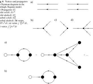
M
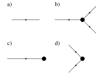
Fig. 1 Feynman diagram components for (a) an edge, the propagatorG(t, t), and vertices (b)bxx˜ 2dt,
(c)yxδ(t˜ −t0) dt, and
(d) D2x˜2dt
product ofNvvertices. Each term in this expansion corresponds to a graph withNv
interior vertices. We label thekth vertex with timetk. As indicated in equation (25),
there is an integration over each such interior time point, over the interval(t0,∞).
The interactionVnmproduces vertices withnedges to the left of the vertex (towards
increasing time) andmedges to the right of the vertex (towards decreasing times). Edges between vertices represent propagators that arise from an application of Wick’s theorem and thus everyx(t˜ )must be joined by a factor ofx(t )in the future, i.e.t > t, becauseG(t, t)∝H (t−t). Also, sinceH (0)=0 by the Ito condition, each edge must connect two different vertices. All edges must be connected, a vertex for the interactionVnmmust connect tonedges on the left andmedges on the right.
Hence, terms at theNvth order of the expansion for the moment
N
j=1x(tj)×
M
k=1x(t˜ k) are given by directed Feynman graphs withN final endpoint vertices,
Minitial endpoint vertices, andNvinterior vertices with edges joining all vertices in
all possible ways. The sum of the terms associated with these graphs is the value of the moment toNvth order. Figure1shows the vertices applicable to action (20) with
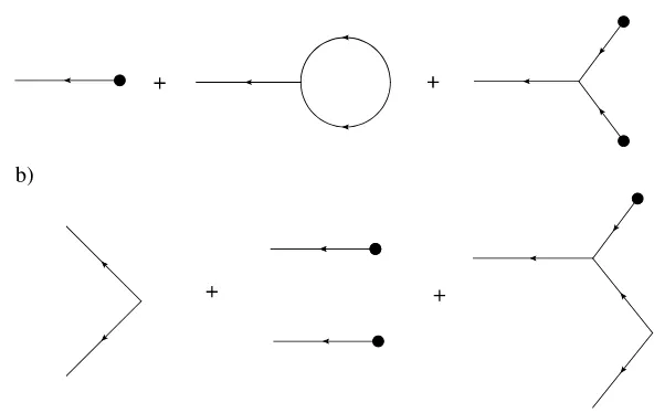
p=0. Arrows indicate the flow of time, from right to left. These components are combined into diagrams for the respective moments. Figure2shows three diagrams in the sum for the mean and second moment ofx(t ). The entire expansion for any given moment can be expressed by constructing the Feynman diagrams for each term. Each Feynman diagram represents an integral involving the coefficients of a vertex and propagators. The construction of these integrals from the diagram is encapsulated in the Feynman rules:
(A) For each vertex interactionVnmin the diagram, include a factor of−vnnm! . The
minus sign enters because the action appears in the path integral with a minus sign. (B) If the vertex type,Vnmappearsktimes in the diagram, include a factor ofk1!.
(C) For each edge between timest andt, there is a factor ofG(t, t).
(D) Forndistinct ways of connecting edges to vertices that yield the same dia-gram, i.e. the same topology, there is an overall factor ofn. This is the combinatoric factor from the number of different Wick contractions that yield the same diagram.
(E) Integrate over the timest of each interior vertex over the domain(t0,∞).
Fig. 2 Feynman diagrams for (a) the mean and (b) second moment for action (20) withp=0
parameterα. Each appearance of that particular vertex diagram contributes a factor ofα and the expansion can be continued to any order in α. The expansion is also generally valid over all time ifG(t, t)decays exponentially for larget−tbut can break down if we are near a critical point andG(t, t)obeys a power law. We consider the semiclassical expansion in the next section where the small parameter is the noise strength.
Comparing these rules with the diagrams in Fig.2, one can see the terms in the expansions in equations (23) and (24), with the exception of the middle diagram in Fig.2b. An examination of Fig.2a shows that this middle diagram consists of two copies of the first diagram of the mean. Topologically, the diagrams have two forms. There are connected graphs and disconnected graphs. The disconnected graphs repre-sent terms that can be completely factored into a product of moments of lower order (cf. the middle diagram in Fig.2b). Cumulants consist only of connected graphs since the products of lower ordered moments are subtracted by definition. The connected diagrams in Fig.2lead to the expressions (23) and (24). In the expansion (21), the terms that do not include the source factorsJ andJ˜only contribute to the normal-izationZ[0,0]and do not affect moments because of (18). In quantum field theory, these terms are called vacuum graphs and consist of closed graphs, i.e. they have no initial or trailing edges. In the cases we consider, all of these terms are 0 if we set
Z[0,0] =1.
4.3 Semiclassical Expansion
Recall that the action for the general SDE (3) is
S[x,x˜] =
˜
xx˙−fx(t ), t−D
2x˜
where we make explicit a small noise parameterD, whilef andgare of order one. Now, rescale the action with the transformationx˜→ ˜x/Dto obtain
S[x,x˜] = 1 D
˜
xx˙−fx(t ), t−1
2x˜
2g2x(t ), tdt.
The generating functional then has the form
Z[J,J˜] =
Dx(t )Dx(t )e˜ −(1/D)(S[x(t ),x(t )˜ ]−
˜
J (t )x(t ) dt−J (t )x(t ) dt )˜ . (26)
In the limit asD→0, the integral will be dominated by the critical points of the exponent of the integrand. In quantum theory, these critical points correspond to the “classical” equations of motion (mean field theory in statistical mechanics). Hence, an asymptotic expansion in smallDcorresponds to a semiclassical approximation. In both quantum mechanics and stochastic analysis this is also known as a WKB expansion. According to the Feynman rules for such an action, each diagram gains a factor ofDfor each edge (internal or external) and a factor of 1/Dfor each vertex. LetEbe the number of external edges,I the number of internal edges, andV the number of vertices. Then each connected graph now has a factorDI+E−V. It can be shown via induction that the number of closed loopsLin a given connected graph must satisfyL=I−V+1 [26]. To see this, note that for diagrams without loops any two vertices must be connected by at most one internal edge since more than one edge would form a closed loop. Since the diagrams are connected we must haveV =I+1 whenL=0. Adding an internal edge between any two vertices increases the number of loops by precisely one. Thus we see that the total factor for each diagram may be writtenDE+L−1. Since the number of external edges is fixed for a given cumulant, the order of the expansion scales with the number of loops.
We can organize the diagrammatic expansion in terms of the number of loops in the graphs. Not surprisingly, the semiclassical expansion is also called the loop ex-pansion. For example, as seen in Fig.2a the graph for the mean has one external edge and thus to lowest order (graph with no loop), there are no factors ofD, while one loop corresponds to the orderDterm. The second cumulant or variance has two ex-ternal edges and thus the lowest order tree level term is orderDas seen in Fig.2b. Loop diagrams arise because of nonlinearities in the SDE that couple to moments of the driving noise source. The middle graph in Fig.2a describes the coupling of the variance to the mean through the nonlinearx2term. This produces a single-loop dia-gram which is of orderD, compared to the order 1 “tree” level mean graph. Compare this factor ofDto that from the tree level diagram for the variance, which is orderD. This same construction holds for higher nonlinearities and higher moments for gen-eral theories. The loop expansion is thus a series organized around the magnitude of the coupling of higher moments to lower moments.
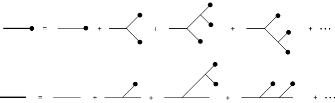
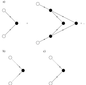
Fig. 3 Bold edges represent the sum of all tree level diagrams contributing to that moment. (Top) The meanx(t )tree. (Bottom) Linear responseGtree(t, t)
set of self-consistent equations. For example, consider the expansion of the mean for action (20) for the case whereD=0 (i.e. no noise term). The expansion will consist of the sum of all tree level diagrams. From Eq. (23), we see that it begins with
x(t )=yG(t, t0)+by2
G(t, t1)G(t1, t0)2dt1+ · · ·.
In fact, this expansion will be the perturbative expansion for the solution of the ordi-nary differential equation obtained by discarding the stochastic driving term. Hence, the sum of all tree level diagrams for the mean must satisfy
d
dt
x(t )tree= −ax(t )tree+bx(t )2tree+yδ(t−t0). (27)
Similarly, the sum of the tree level diagrams for the linear response,x(t )x(t˜ )tree= Gtree(t, t), is the solution of the linearization of (27) around the mean solution with a unit initial condition att=t, i.e. the propagator equation
d dtGtree
t, t= −aGtreet, t+2bx(t )treeGtreet, t+δt−t. (28) The semiclassical approximation amounts to a small noise perturbation around the solution to this equation. We can represent the sum of the tree level diagrams graphi-cally by using bold edges, which we call “classical” edges, as in Fig.3. We can then use the classical edges within the loop expansion to compute semiclassical approxi-mations to the moments of the solution to the SDE.
Consider the case ofp=0 in action (20). The one-loop semiclassical approxi-mation of the mean is given by the sum of the first two graphs in Fig.2a with the thin edges replaced by bold edges. For the covariance, the first graph in Fig.2b suf-fices, again with thin edges replaced by bold edges. These graphs are equivalent to the equations:
x(t )=x(t )tree+bD
t
t0
dt1
t1
t0
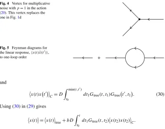
Fig. 4 Vertex for multiplicative noise withp=1 in the action (20). This vertex replaces the one in Fig.1d
Fig. 5 Feynman diagrams for the linear response,x(t )x(t˜ ), to one-loop order
and
x(t )xtC=D
min(t,t) t0
dt1Gtree(t, t1)Gtree
t, t1
. (30)
Using (30) in (29) gives
x(t )=x(t )tree+bD
t
t0
dt1Gtree(t, t2)x(t2)x(t2)C.
This approximation is first order inDfor the mean (one loop) and covariance (tree level).
Now consider the one-loop corrections whenp=1 in action (20). First consider the linear response,x(t )x(t˜ ). For simplicity, we will assume the initial condition
y=0. In this case, the vertex in Fig.1d now appears as in Fig.4. The linear response
x(t )x(t˜ ) will be given by the sum of all diagrams with one entering edge and one exiting edge. At tree level, there is only one such graph, equal toG(t, t), given in (22). At one-loop order, we can combine the vertices in Figs.1b and1d to get the second graph shown in Fig.5to obtain
x(t )x˜t=Gt, t+bD
dt1dt2G(t, t2)G(t2, t1)2Gt2, t =e−a(t−t)Ht−t1+bD
t−t
a +
1
a2
e−a(t−t)−1.
Combining the diagrams in Figs.1 and4, the analog to Eqs. (29) and (30) for
p=1 are
x(t )=x(t )tree+bD
t
t0
dt1
t1
t0
dt2Gtree(t, t2)Gtree(t2, t1)2
x(t )tree (31)
and
x(t )xtC=D
min(t,t) t0
dt1Gtree(t, t1)Gtreet, t1x(t )tree. (32) Using the definition of Gtree(t, t), the self-consistent semiclassical approximation forx(t )to one-loop order is
d dt
x(t )+ax(t )−bx(t )2=bD
t
t0
dt1Gtree(t, t1)2
x(t )
or
d dt
x(t )+ax(t )−bx(t )2=b
t
t0
dt1x(t1)x(t1)C.
The semiclassical approximation known as the “linear noise” approximation takes the tree level computation for the mean and covariance. The formal way of deriving these self-consistent equations is via the effective action, which is beyond the scope of this review. We refer the interested reader to [26].
An alternative way of deriving the loop expansion equations is to examine devia-tions away from the mean directly by transforming to a new variablez=x− ¯xwhere
¯
xdef= x(t )treesatisfies the SDE with zero noise (27). The action then becomes
S[x,x˜] =
dtx˜z˙+az−2xz¯ −bz2− ˜x2(z+ ¯x)pD
2. (33) The propagator for this action is now given immediately by (28). At tree level,
ztree=0 by definition. At order D, the mean is given by the second diagram in Fig.2a, which immediately gives (29) and (31). Likewise, the variance will be given by the diagram in Fig.1d leading to (30) and (32).
5 FitzHugh–Nagumo Model
These methods can also be applied to higher dimensions. As an example, consider the noise-driven FitzHugh–Nagumo neuron model:
˙
v=v−1
3v
3−w+I+v
0δ(t−t0)+ √
Dη(t ), (34)
˙
w=c(v+a−bw)+w0δ(t−t0), (35)
a semiclassical or WKB expansion in terms ofD. We wish to compute the means, variances, and covariance forvandwas a loop expansion inD.
We first must formally construct a joint PDF for variablesvandw. As both equa-tions in the system must be satisfied simultaneously, we write
Px(t )|y, t0=
Dη(t )δ
˙
v−v+1
3v
3+w−I−√Dη(t )−v0δ(t−t0)
×δw˙ −c(v+a−bw)−w0δ(t−t0)e−Sη[η(t )],
which leads to the action
S= v˜
˙
v−v+1
3v
3+w−I−√Dη(t )−v
0δ(t−t0)
−D
2v˜
2
+ ˜ww˙−c(v+a−bw)−w0δ(t−t0)dt.
We now transform to deviations around the mean withν=v−V andω=w−W, withV def= vtreeandWdef= wtree, where
˙
V =V −1
3V
3−W+I,
(36)
˙
W =c(V+a−bW ). (37)
The transformed action is
S= v˜
˙
ν−ν+V2ν+V ν2+1
3ν
3+ω
−D
2v˜
2+ ˜wω˙−c(ν−bω)dt
which we can rewrite as
S= ψ˜T(t )·G−1t, t·ψtdt+ ˜vV ν2+1
3vν˜
3−D
2v˜
2
dt, (38)
where
ψ=
ν ω
, ψ˜ =
˜ v ˜ w
,
G−1t, t=
(dtd +V2−1)δ(t−t) δ(t−t) −cδ(t−t) (dtd +cb)δ(t−t)
.
The propagator
Gt, t=
Gvν(t, t) Gwν(t, t) Gvω(t, t) Gwω(t, t)
satisfies
G−1t, tGt, tdt=
δ(t−t) 0 0 δ(t−t)
Fig. 6 Vertices and propagators for Feynman diagrams in the Fitzhugh–Nagumo model. (a) PropagatorsGvν
(solid–solid),Gνw
(solid–dashed),Gvω
(dashed–solid),Gwω
(dashed–dashed), (b) vertex
˜
vV ν2dt, (c) vertex D2v˜2dt, (d) vertex 13vν˜ 2dt
Fig. 7 (a) Diagrammatic expansion for the mean ofv(t ), showing the one-loop and an example two-loop graph. (b) Diagrams forw(t )are topologically identical with the replacement of the leftmost line by the
Gvω(t, t)propagator
or
d dt +V
2−1
Gvν+Gvω=δt−t, (39)
d
dt +cb
Gvω−cGvν =0, (40)
d dt +V
2−
1
Gwν +Gwω =0, (41)
d dt+cb
Gwω−cGwν =δt−t. (42)
The Feynman diagrams for the four propagators (39)–(42) and the two vertices in the action (38) are shown in Fig.6.
Fig. 8 (a) Diagrammatic expansion for the two-point correlationv(t )v(t), showing the tree level and an example one-loop graph. Diagrams for (b)w(t )w(t)and (c)v(t )w(t)are topologically identical with the replacement of the appropriate external lines by theGvω(t, t)propagator
diagram in Fig.2a:
ν(t )
t0= −D t
t0
dt1
t
t0
dt2V (t )Gvν(t, t2)Gvν(t2, t1)Gvν(t2, t1), (43)
where the subscript indicates that this is an ensemble average ofν(t )in the domain
[t0, t].ωis given by the same diagram asνexcept that propagatorGvω(t, t2)
re-placesGvν(t, t2):
ω(t )t
0= −D t
t0
dt1
t
t0
dt2V (t )Gvω(t, t2)Gvν(t2, t1)Gvν(t2, t1). (44)
The diagrams for the variances and covariances (two-point cumulants) are shown in Fig.8The variance ofvisν(t )ν(t)Cin Fig.8a is found by using Fig.6c adjoined
to twoGvν propagators:
Cνν
t, t;t0
def
=ν(t )νtC=D
min(t,t) t0
dt1Gvν(t, t1)Gvν
t, t1
The variance ofwisω(t )ω(t)Cin Fig.8b is also given by Fig.6c but adjoined to
twoGvωpropagators:
Cωω
t, t;t0def=ω(t )ωtC=D
min(t,t) t0
dt1Gvω(t, t1)Gvωt, t1. (46)
Finally, the covariance of v andw isν(t )ω(t)C in Fig. 8c is given by Fig. 6c
adjoined to theGvν andGvωpropagators:
Cνω
t, t;t0
def
=ν(t )ωtC=D
min(t,t) t0
dt1Gvν(t, t1)Gvω
t, t1
. (47)
To evaluate these expressions we first solve the deterministic equations (37) to ob-tainV (t )andW (t ). We then useV (t )in (39)–(42) and solve for the four propagators, which go into the expressions for the moments. When the solutions of (37) are fixed points, then we can find closed-form solutions for all the equations. Otherwise, we may need to solve some of the equations numerically. However, instead of having to average over many samples of the noise distribution, we only need to solve a small set of equations once to obtain the moments.
Here we give the example solution for the fixed point given by the solution of
0=V −1
3V
3−W+I, (48)
0=c(V+a−bW ). (49)
The propagator equations are pairwise coupled and thus can easily be solved by Laplace transforms or any other means to obtain
Gvνt, t=e−r(t−t)
cosΩt−t−r−bc Ω sin
Ωt−tHt−t, (50)
Gvωt, t= c Ωe
−r(t−t)
sinΩt−tHt−t, (51)
Gwνt, t= 1 Ωe
−r(t−t)sinΩt−tHt−t, (52)
Gwωt, t= −e−r(t−t)
cosΩt−t+r−bc Ω sin
Ωt−tHt−t, (53)
wherer=(1/2)(V2−1+bc),
Ω=(1/2)−V4+2(1+bc)V2−b2c2−2(b−2)c−1.
We can now insert these propagators into the variance and covariance equations:
ν(t )t
0= −DV t
t0
dt2e−r(t−t2)
cosΩ(t−t2)−r−2bc
2Ω sin
Ω(t−t2)
×
t2
t0
×
cosΩ(t2−t1)
−r−bc Ω sin
Ω(t2−t1)
2
, (54)
ω(t )t
0= −DV
c Ω
t
t0
dt2e−r(t−t2)sin
Ω(t−t2)
×
t2
t0
dt1e−2r(t2−t1)
×
cosΩ(t2−t1)
−r−bc Ω sin
Ω(t2−t1)
2
, (55)
Cνν
t, t;t0=D
min(t,t) t0
dt1e−r(t−t1)
×
cosΩ(t−t1)
−r−2bc
2Ω sin
Ω(t−t1)
(56)
×e−r(t−t1)
cosΩt−t1−r−2bc
2Ω sin
Ωt−t1, (57)
Cωω
t, t;t0
=D c 2 Ω2
min(t,t) t0
dt1e−r(t−t1) ×sinΩ(t−t1)
e−r(t−t1)sinΩt−t
1
, (58)
Cνω
t, t;t0=Dc Ω
min(t,t) t0
dt1e−r(t−t1)
×
cosΩ(t−t1)
−r−2bc
2Ω sin
Ω(t−t1)
(59)
×e−r(t−t1)sinΩ(t−t1). (60)
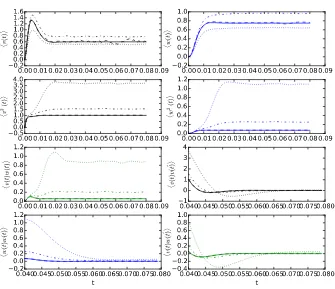
These expressions not only capture the stationary values but also transient effects. The integrals can all be performed in closed form and result in long expressions of exponential and trigonometric functions, which we do not include here. Figure9
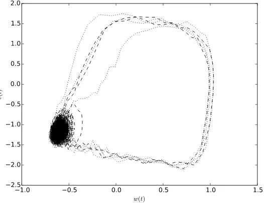
shows the comparison between these perturbative estimates and numerical simula-tions for three different noise values,D=0.001,0.01,0.015. We used the parame-tersa=0.7,b=0.8,c=0.1,I =0, which give rise to fixed pointsV = −1.1994 andW= −0.62426 and propagator parametersr=0.25928 andΩ=0.26050. Nu-merical simulations are averages over one million samples. The estimates fit the data extremely well forD=0.001 but start to break down forD=0.01. The reason is that the perturbation expansion is only valid in the vicinity of the fixed point but as the noise strength increases the probability to escape from the fixed point and enter an excitable orbit becomes significant. Phase plane portraits in Fig.10show that for
Fig. 9 Comparison of ensemble average simulations vs. analytic expansions for the Fitzhugh–Nagumo model. For each moment, we show the one-loop (for the mean) or tree (for the two-point cumulants) level approximation (solid line) along with simulations forD=0.001 (dashed line),D=0.01 (dot–dashed line), andD=0.015 (dotted line). Means have been scaled byDV and two-point cumulants have been scaled byDso they can be compared directly
and WKB theory as detailed in [13,25]. Software for performing simulations and integrals is available upon request.
6 Connection to Fokker–Planck Equation
In stochastic systems, one is often interested in the PDF p(x, t ), which gives the probability density of positionx at timet. This is in contrast with the probability density functionalP[x(t )]which is the probability density of all possible functions or pathsx(t ). Previous sections have been devoted to computing the moments of
P[x(t )], which provide the moments ofp(x, t )as well. In this section we leverage knowledge of the moments ofp(x, t ) to determine an equation it must satisfy. In simple cases, this equation is a Fokker–Planck equation forp(x, t ).
The PDFp(x, t )can be formally obtained fromP[x(t )]by marginalizing over the interior points of the functionx(t ). Consider the transition probabilityU (x1, t1|x0, t0)