http://www.sciencepublishinggroup.com/j/ajcst doi: 10.11648/j.ajcst.20190203.11
ISSN: 2640-0111 (Print); ISSN: 2640-012X (Online)
Edge Detection of an Image Based on Extended Difference
of Gaussian
Hameda Abd El-Fattah El-Sennary
1, *, Mohamed Eid Hussien
1, Abd El-Mgeid Amin Ali
21
Faculty of Science, Aswan University, Aswan, Egypt
2Faculty of Computers and Information, Minia University, Minia, Egypt
Email address:
*
Corresponding author
To cite this article:
Hameda Abd El-Fattah El-Sennary, Abd El-Mgeid Amin Ali, Mohamed Eid Hussien. Edge Detection of an Image Based on Extended Difference of Gaussian. American Journal of Computer Science and Technology. Vol. 2, No. 3, 2019, pp. 35-47.
doi: 10.11648/j.ajcst.20190203.11
Received: November 24, 2019; Accepted: December 9, 2019; Published: December 20, 2019
Abstract:
Edge detection includes a variety of mathematical methods that aim at identifying points in a digital image at which the image brightness changes sharply or, more formally, has discontinuities. The points at which image brightness changes sharply are typically organized into a set of curved line segments termed edges. The same problem of finding discontinuities in one-dimensional signals is known as step detection and the problem of finding signal discontinuities over time is known as change detection. Edge detection is a fundamental tool in image processing, machine vision and computer vision, particularly in the areas of feature detection and feature extraction. It's also the most important parts of image processing, especially in determining the image quality. There are many different techniques to evaluate the quality of the image. The most commonly used technique is pixel based difference measures which include peak signal to noise ratio (PSNR), signal to noise ratio (SNR), mean square error (MSE), similarity structure index mean (SSIM) and normalized absolute error (NAE).... etc. This paper study and detect the edges using extended difference of Gaussian filter applied on many of different images with different sizes, then measure the quality images using the PSNR, MSE, NAE and the time in seconds.Keywords:
Edge Detection, Image Quality, Gaussian Filter, Extended Difference of Gaussian, Peak Signal to Ratio, Mean Square Error1. Introduction
Machine vision has developed into a critical field embracing a wide range of applications, comprehensive robot assembly [1], traffic monitoring and control [2], biometric measurement [3], surveillance [4], analysis of remotely sensed images [5], automated inspection [6], vehicle guidance [7] and signature verification [8]. The work in this field is still documented by researchers and specialists. The early stages of vision, handling distinguish highlights in images that are important to estimate the Properties and structure of elements in the scene [9]. Edges are one such component. It is great nearby changes in the image [10], the active components for investigating images. It usually happens in the limit between two unique areas in the image.
are often non-friable when they are extracted from non-trivial images [14], as a result, we get disconnected edges and lose slices from the edge as well as false edges not compatible with interesting phenomena in the image. The edges extracted in a three - dimensional scene of a two - dimensional image are divided into two types are a dependent view or an independent view. The independent view of the discovery of the edges usually fluctuates the established characteristics of the three-dimensional objects, such as surface shape and surface marks [15]. The edge of the view may change according to the change of view, and typically inverting the geometry of the scene, such as objects occluding one another [16]. Edges are coming across in the areas of feature extraction and feature selection in Computer Vision. In edge detection algorithm we enter the digital image, as input and exit the edge map as output. Many detectors have been introduced in the previous works such as canny, log, zerocross, Sobel, approxcanny, Roberts and Prewitt [17-23].
The purpose of this research is to detect and improve the edge information existing in the image, since it is important to understand the image and see what information it contains. This paper organized as follow: section 2 introduces a look at some of the classical methods of edge detection. Section 3 will get to know Gaussian filter and its theory, and in addition to its function. Difference of Gaussian and its extended presented in 4,5.
In section 6 provide the effectiveness of our methods when applied many of images that have different sizes. Finally, we introduce the conclusion of this paper in section 7.
2. Some of Classical Methods for
Detecting Edges
2.1. Canny Edge Detector
Canny edge detection is a technique used to significantly reduce the amount of information processed and thus obtain only important information. It has been widely applied in different computer vision systems. Canny found that there was a relative similarity in the requirements for applying edge detectors to different vision systems.
Process of Canny Edge Detection Algorithm
The canny edge detection algorithm can be divided into five steps [24]:
Step. 1 In order to remove noise from the image and soften it, we apply the Gaussian filter.
Step. 2 We extract the gradients of the intensity of the image. Step. 3 apply non- maxima suppression to get edge response from one side.
Step. 4 To discover the edge and be connected, we use the double threshold method.
Step. 5 The final step in detecting edges is to dispense with all weak edges that are
Not connected to strong edges.
2.2. Log Filter
The edge detection based on log filter consists of three steps. The first step is Gaussian filtering, the second is edge enhancement and the three step is the edge detection. The Laplacian operator is used for enhancement and detect the edges [25] but it's sensitive to the noise. In order to reduce noise effects, the image firstly is smoothed, then is detected for edge by Laplacian operator. The optimal smoothing filter should have good characteristics in the spatial domain and frequency domain at the same time.
2.2.1. Linear Filters
Let , for , , = 1, … … , , are the values for of the pixels in the image and if we
Assume the linear filter has a size 2 + 1 2 + 1 and the weights are where , = − , … … . , is shown by the following equation
∑"#$"∑"#$" ,!
,
, % = + 1 , … . . , − (1)An image can be represented in a different way like a synthesis of different sine waves in frequency rather than as a matrix [26]. This refers to the Fourier representation. The Fourier coefficients are determined from the coefficients that determine sine waves. For engineers and some researchers this is obvious to them, but for others it maybe takes some times to get used to it.
2.2.2. Non Linear Edge Detection Filters
There are some of simple, non linear filters for detecting edges in all directions [27] such as:
1)The difference between large and small values results in a filter that represents an output for the range of pixel values.
= & ' ( , (: , = − , … … , * − ' ( , (: , =
− , … . * (2)
The filter is simple and fast at work and we can get it by adjusting the moving average algorithm. Alternatively, this filter can be processed by using the property that splits both the maximum and minimum values.
2)Roberts detector is known as the sum of the differences in the absolute values of diagonally opposite pixel values
= + − (,, (,+ + | (,, − , (,| (3)
3)the kirch filter is one of the form conformity filters, in which the filter output is the maximum response from a group of linear filters that are sensitive to edges in different directions
= max1 ,,..2∑, 3,∑, 3, 1 ( , ( (4)
, = 4 −3 0 − 35 5 5
−3 − 3 − 3 8
,
9 = 4 5 5 − 35 0 − 3
−3 − 3 − 3 8
: = 45 − 3 − 35 0 − 3
5 − 3 − 3 8 (5) And each subsequent weight matrix, ; ,……. 2 has elements which are successively rotated through multiples 45. This is a much slower algorithm compared to the two previous methods. To minimize the impact of noise, using gradient filters which is one of the best ways to do this.
The gradient filters such as: a) Prewitt filter
<=>> ?9+ =>>@ ?9
We can design the filter to count the gradient by substituting partial derivatives by equation (10)
>
> =16 B 3,, (, , (, (,, (, 3,, 3, , 3, (,, 3,C D !
DE ,
FB (,, 3, (,, (,, (, 3,, 3, 3,,
3,, (,C (6)
b) Sobel is comparable to Prewitt filter, except when evaluating the largest gradation. It presents greater weight to
the pixels near to , % as follow
>
> 18 B 3,, (, 2 , (, (,, (, 3,, 3, 2 , 3,
(,, 3,C
D ! DE
,
2B (,, 3, 2 (,, (,, (, 3,, 3, 2 3,,
3,, (,C (7)
2.3. Zero - Crossing Edge Detector
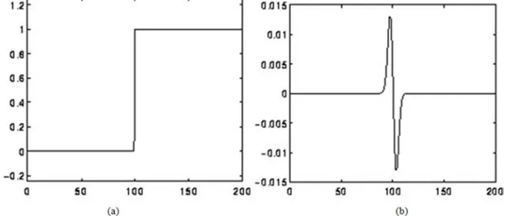
The value of the Laplacian passes through zero, so the zero crossing looking for places in the Laplacian of an image. There are points in the image where there is a rapid change in the intensity and this is possible occurs at the edges of the image and possible occurs in places not easy to connect to the edges. We can say that the zero crossing detector is used to store some features and not only the edge detector. Zero crossing is always located on closed oceans, so the output is a single-pixel binary image with thick lines showing the point positions of the zero crossing. The zero crossing edge detector starts with the image filtered by Laplacian of Gaussian [28]. The results from zero sections are highly influenced by the size of Gaussian that used in the smoothing phase. When heterogeneity increases, we get less zero crossing contours, which correspond to the largest range in the image. In the LoG output, edges in images lead to zero crossings
.
Figure 1. Utilization step edge in a 1-D log filter. (a) Define a 1-D image, includes Step edge. (b) Indicate 1-D LoG filter with Gaussian deviation 3 pixels
Laplacian of Gaussian
The Laplacian is a Two - dimensional proportional scale of the 2nd spatial derivative of an image. The Laplacian of an image indicates areas of rapid change in density and is therefore often used for edge detection. The image should be smoothed first by using something like a Gaussian filter to reduce its sensitivity to noise and then apply the Laplacian. The operator normally takes a single gray level image as input and produces another gray level image as output.
The Laplacian , @ of an image with pixel intensity values H , @ is given by
, @ DKDIJI D IJ
DEI (8)
Because the image is represented as a set of separate pixels, we must identify a separate torsion nucleus that can approximate the second derivatives in the definition of the Laplacian. Two small kernels are shown in figure 2.
Figure 2. Two approximations for Laplacian.
they are. To register this, the image is often used Gaussian smoothed before using the Laplacian filter. Before the differentiation step we must do the pre-processing step because it reduces the high frequency noise components.
We can convolve the Laplacian filter with the Gaussian smoothing filter because the convolution operation is connected, and then convolve the resulting filter with the image to get the desired result. Working this way has two advantages:
i. Gaussian kernel and the Laplacian kernel are usually smaller than the image. So this method requires small calculations.
ii. At run time we need one convolution to be performed because the kernel of Log can be calculated at the beginning.
iii.The 2-D LoG function centered on zero and with Gaussian standard deviationL has the form
LOG , @ PQ,IR1 K I(EI 9QI S T3
UI VI
IWI (9)
Figure 3. The 2D-Laplacian of Gaussian function. x and y axes are marked in standard deviation.
A separate kernel that explained in the equation (9) (for Gaussian 1.4 ) is shown in figure 4
Figure 4. Log function with Gaussian L 1.4.
3. Gaussian Filter
Gaussian filter is a framework filter of linear layer [29], it means weighted mean. Because weights in the filter calculated according to a Gaussian distribution, it's named
after famous scientist Carl Gauss. This filter has another name is Gaussian blur.
3.1. Gaussian Blur Theory
We can clarify the blur as taking a pixel as the average value of its surrounding pixels. If we assume the center point is 2, the surrounding points are 1 and the center point will take the average value of its surrounding points, it will be 1. If every point will get the average value of surrounding points, then how should we allocate weight?. If we just use simple average, it's unreasonable, because images are continuous, the closer the points in the distance, the closer the relationship between points. Hence the weighted average is more logical than the simple average, the closer the points in the distance, the larger the weight.
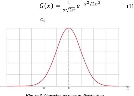
3.2. Gaussian Function
The density function calls the Gaussian function. The 1-D shape is shown in the following equation
Y
Q√9P,T
3 K3[ I/9QI(10)
Here & is the average of , Because center point is both point origin when calculating an average value, so & equals to 0
.
Y
Q√9P,T
3KI/9QI(11)
Figure 5. Gaussian or normal distribution.
Thus the function is negative exponential one of squared argument. Argument divider L plays the role of scale factor. L Parameter has a special name: standard deviation, and its square L9. Pre multiplier in front of the exponent is selected the area below plot to be 1. The function is marked everywhere on real axis ∈ ∞, ∞ Which means it spreads endlessly to the left and to the right.
Figure 6. Gaussian distribution truncated at points a3L.
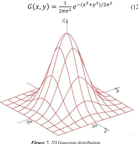
Based on the one dimensional function, we can derive the two dimensional Gaussian function
Y
, @
9PQ, IT
3 KI(EI /9QI
(12)
Figure 7. 2D Gaussian distribution.
Gaussian distribution has precious property. See equation (12) could be rewritten as follows:
Y , @ 9PQ,IT3 K
I(EI/9QI , 9PQIT3K
I/9QI , 9PQIT3E
I/9QI
Y Y @ (13) Which means 2D distribution is divided into a pair of 1D ones, and so, 2D filter window is separated into a pair of 1D ones. In this case the filter is called separable one.Practically it means that to apply a filter to an image it is enough to filter it in the horizontal direction with 1D filter and then the result is filtered in vertical direction with the same filter. Which direction first really makes no difference.
2D Gaussian separable algorithm i. Calculate 1D window weights
ii. Every image line is filtered as 1D signal
iii.Every filtered image column is filtered as 1D signal
4. Difference of Gaussian (DoG)
In imaging science, difference of Gaussians (DoG) is an enhanced algorithm feature that includes the subtraction of one blurred version of an original image from another, less blurred version of the original [30]. When convolving the original grayscale images with Gaussian kernels having differing standard deviations, we obtain to the blurred images in the simple case of grayscale images. High-frequency spatial information suppresses only when an image blurred using a Gaussian kernel. The spatial information that lies between the ranges of frequencies are saved when subtracting one image from the other. Thus, the difference of Gaussians is a band-pass filter where there are some of spatial frequencies are existing in the original grayscale image but the rest is ignored.
The mathematical formula of difference of Gaussians explained as follows:
Given an image its dimension is b H: cd ⊆ fgh → cj ⊆ fkh
If we have an imageH, the difference of Gaussians (DoG) function of this image is
гQmQI: cd ⊆ fgh → cn ⊆ fh
Obtained by subtracting the image H convolved with the Gaussian of variance L99From the image H convolved with a Gaussian of narrower variance L,9, with L9o L,. In one Dimension, г is defined as:
гQmQI H ∗
, Qm√9PT
3 KI/ 9QmI
H ∗QI√9P, T3 KI/ 9QII
(14)
And for the centered of two dimensional case
гQ, Q , @ H ∗9PQ,IT3 K
I(EI/ 9QI H ∗ , 9PIQIT3 K
I(EI/ 9IQI
(15)
Which is equivalent to
гQ, Q , @ H ∗ 9PQ,IT3 K
I(EI/ 9QI , 9P IQIT3
UI VI I IWI (16)
Which represents an image convoluted to the difference of two Gaussians.
5. Extended Difference of Gaussian
(XDOG)
The difference of Gaussian filter is as follows [31]:
qQ, YQ Y Q r 1 L9s9Y (17)
We need to generate an edge image, if we assume an image may be realized as a thresholding of the DoG response t∈ qQ, ∗ H where
t∈ u cv wxyz{|}~z , •€∈ (18)
Where ∈ is used to Controls noise sensitivity
and models presented by Young and others created edge images using a DoG diverse in which the strength of the inhibitory effect of the larger Gaussian is allowed to vary, which leads to the following equation
D‚,ƒ,„ x G‚ x τ. Gƒ‚ x (19)
After exchanging the binary thresholding function T∈ With a continuous slope:
T∈,‡ u c,(x‰ŠyB‡. •3∈ C wxyz{|}~z , •€∈ (20)
T∈,‡ D‚,ƒ,„∗ I is referring to the XDOG filter for image I
We must know the XDOG is hard to control. Increasing the sensitivity of the filter to edges requires adjusting τ, φ, ∈ well
In order to simplify the difficulties in controlling XDOG using the following equation
S‚,ƒ,Ž x 1 • . G‚ x •. Gƒ‚ x (21) φ control the sharpness in the black and white transformations in the image.
6. Results and Discussion
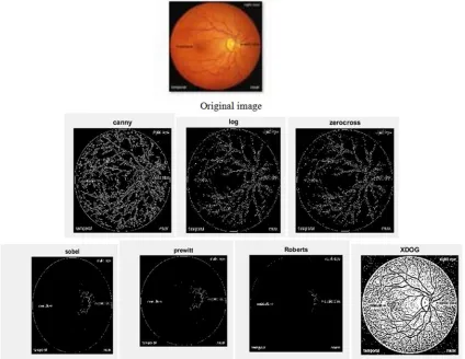
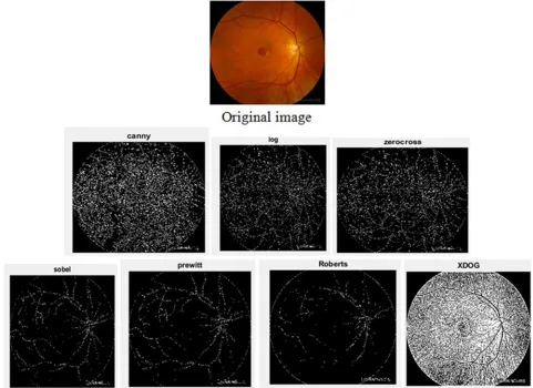
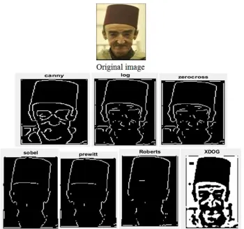
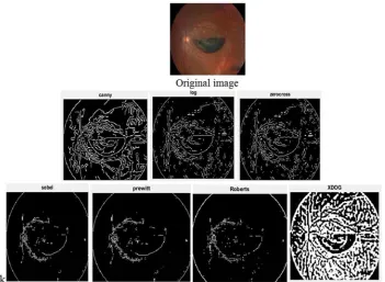
In order to test our method in this paper and compare it with the other classical methods, many of different test images with different sizes and resolutions are detected by canny, log, zerocross, sobel, prewitt and Roberts and XDOG method.
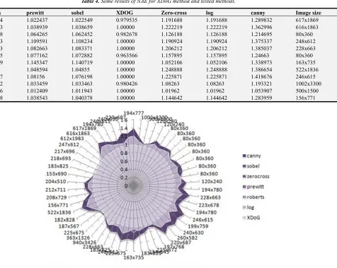
All experiments are executed on a Windows-based machine with Intel (R) Core (TM) i7-7500U [email protected] processor, 16GB RAM, and MATLAB R2017a installed on it. The method tested on 160 image with different sizes and compared with most of known edge detection and we run it 10 times for each image. As shown in figures 8-18 and in tables 1-4 XDOG method works effectively for different images, especially when applied image quality measurements such as Peak Signal to Noise Ratio (PSNR), Mean Square Error (MSE), Normalized Absolute Error (NAE) and finally compared with Time in seconds. From Table 1, 2 and Table 4 can observe that, PSNR, MSE, NAE obtained with the proposed method is better compared with the classical methods especially canny, log, zero-cross. But from table 3 can observe that the time for XDOG method is relatively large. In the end, we can say our method is better than all tested methods.
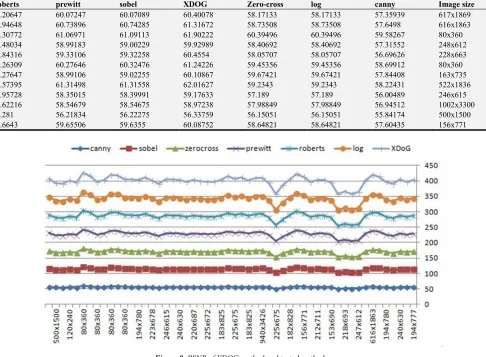
Table 1. Some results of PSNR for XDOG and tested methods.
Roberts prewitt sobel XDOG Zero-cross log canny Image size
60.20647 60.07247 60.07089 60.40078 58.17133 58.17133 57.35939 617x1869
60.94648 60.73896 60.74285 61.31672 58.73508 58.73508 57.6498 616x1863
61.30772 61.06971 61.09113 61.90222 60.39496 60.39496 59.58267 80x360
59.48034 58.99183 59.00229 59.92989 58.40692 58.40692 57.31552 248x612
59.84316 59.33106 59.32258 60.4554 58.05707 58.05707 56.69626 228x663
60.26309 60.27646 60.32476 61.24226 59.45356 59.45356 58.69912 80x360
60.27647 58.99106 59.02255 60.10867 59.67421 59.67421 57.84408 163x735
61.57395 61.31498 61.31558 62.01627 59.2343 59.2343 58.22431 522x1836
58.95728 58.35015 58.39991 59.17633 57.189 57.189 56.00489 246x615
58.62216 58.54679 58.54675 58.97238 57.98849 57.98849 56.94512 1002x3300
56.281 56.21834 56.22275 56.33759 56.15051 56.15051 55.84174 500x1500
59.6643 59.65506 59.6355 60.08752 58.64821 58.64821 57.60435 156x771
Figure 8. PSNR of XDOG method and tested methods.
methods because it contains the largest possible values and for greater accuracy we applied the method on different images with different sizes and we got the best quality.
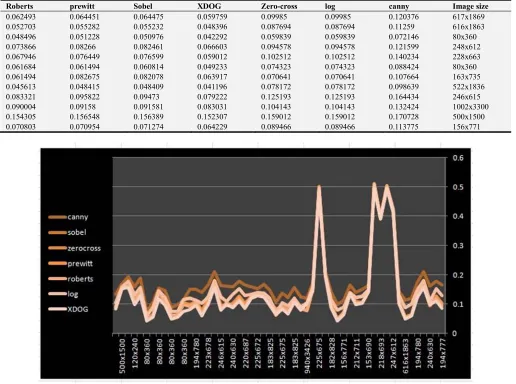
Table 2. Some results of MSE for XDOG and tested methods.
Roberts prewitt Sobel XDOG Zero-cross log canny Image size
0.062493 0.064451 0.064475 0.059759 0.09985 0.09985 0.120376 617x1869
0.052703 0.055282 0.055232 0.048396 0.087694 0.087694 0.11259 616x1863
0.048496 0.051228 0.050976 0.042292 0.059839 0.059839 0.072146 80x360
0.073866 0.08266 0.082461 0.066603 0.094578 0.094578 0.121599 248x612
0.067946 0.076449 0.076599 0.059012 0.102512 0.102512 0.140234 228x663
0.061684 0.061494 0.060814 0.049233 0.074323 0.074323 0.088424 80x360
0.061494 0.082675 0.082078 0.063917 0.070641 0.070641 0.107664 163x735
0.045613 0.048415 0.048409 0.041196 0.078172 0.078172 0.098639 522x1836
0.083321 0.095822 0.09473 0.079222 0.125193 0.125193 0.164434 246x615
0.090004 0.09158 0.091581 0.083031 0.104143 0.104143 0.132424 1002x3300
0.154305 0.156548 0.156389 0.152307 0.159012 0.159012 0.170728 500x1500
0.070803 0.070954 0.071274 0.064229 0.089466 0.089466 0.113775 156x771
Figure 9. MSE of XDOG method and tested methods.
We can observe from table 2 and figure 9 XDOG approach is the perfect compared to the other classical methods where it has the lowest values. These results are the best that can be obtained
Table 3. Some results of time by seconds for XDoG method and tested methods.
Roberts prewitt sobel XDOG Zero-cross log canny Image size
0.03482 0.02890 0.03137 0.14694 0.11677 0.11410 0.11176 617x1869
0.02844 0.02941 0.02965 0.159776 0.10995 0.11125 0.12661 616x1863
0.00485 0.00156 0.00346 0.003816 0.00705 0.00362 0.00675 80x360
0.00335 0.00209 0.00221 0.025025 0.01057 0.01998 0.01906 248x612
0.00315 0.00195 0.00087 0.025307 0.00325 0.02133 0.01747 228x663
0.00018 1.87673 0.00171 0.00567 0.00362 0.00549 0.00523 80x360
3.45591 3.32941 0.00223 0.02202 0.00617 0.01660 0.02240 163x735
0.03982 0.04015 0.03713 0.225196 0.17871 0.17803 0.16881 522x1836
0.00486 0.00518 0.00331 0.01767 0.01685 0.00979 0.01898 246x615
0.09721 0.09783 0.09708 0.49216 0.47284 0.44596 0.41595 1002x3300
0.01778 0.01825 0.02074 0.13806 0.09453 0.08938 0.09874 500x1500
Figure 10. Time of seconds of XDOG method and tested methods.
Table 3 and figure 10 indicating the results of the time used in execution and note the time in our method is relatively large but not large in all images.
Table 4. Some results of NAE for XDoG method and tested methods.
Roberts prewitt sobel XDOG Zero-cross log canny Image size
1.013074 1.022437 1.022549 0.979535 1.191688 1.191688 1.289832 617x1869
1.024353 1.038939 1.038659 1.00000 1.222219 1.222219 1.362996 616x1863
1.044618 1.064265 1.062452 0.982678 1.126188 1.126188 1.214695 80x360
1.049573 1.109591 1.108234 1.00000 1.190924 1.190924 1.375337 248x612
1.042353 1.082663 1.083371 1.00000 1.206212 1.206212 1.385037 228x663
1.078355 1.077162 1.072882 0.963566 1.157895 1.157895 1.24663 80x360
0.981229 1.145347 1.140719 1.00000 1.052106 1.052106 1.338973 163x735
1.02973 1.048594 1.04855 1.00000 1.248888 1.248888 1.386654 522x1836
1.020137 1.08156 1.076198 1.00000 1.225871 1.225871 1.418676 246x615
1.027292 1.033459 1.033463 0.980426 1.08263 1.08263 1.193321 1002x3300
1.005846 1.012409 1.011943 1.00000 1.01962 1.01962 1.053907 500x1500
1.037678 1.038543 1.040378 1.00000 1.144642 1.144642 1.283959 156x771
Figure 11. NAE for XDOG method and tested methods.
Figure 12. edge detection for original image and classical methods 241x627.
Figure 14. Edge detection for original image and classical methods240x960
Figure 16. edge detection for original image and classical methods 120x240.
Figure 18. Edge detection for original image and classical methods 201x750.
7. Conclusion
This paper proposes extended difference of Gaussian technique for edge detection and satisfactory results were produced when compared our method with the classical methods canny, log, sobel, prewitt, Roberts and zerocross. XDOG method works well on different images with different sizes. Then we appreciate the images quality using image quality measurements (PSNR, MSE, NAE and time by seconds) is essential task in digital image processing as it provides a better way for image quality assessment and its improvement. It can be observed that higher the value of PSNR and lower value of MSE are desired results and lower values of NAE and relatively large values of time obtained from XDOG method. From the above we conclude that XDOG method is the best of all methods used
.
References
[1] T. Tang, H. C. Lin, M. Tomizuka,a learning-based framework for robot peg-hole- insertion, proceedings of the ASME 2015 dynamic systems and control conference, 2015, pp. 1-9. [2] N. dharan, S. prakash, S. Seenuvasamurthi, Iot based real time
traffic monitoring and control system for smart cities, IAETSD journal for advanced Research in applied sciences, 5 (4) (2018) 295-306.
[3] A. Sharma, A. Raghuwanshi, V. Sharma, Biometric System- A Review, International Journal of Computer Science and Information Technologies, 6 (5) (2015) 4616-4619.
[4] P. Mishra, G. Saroha,A Study on Video Surveillance System for Object Detection and Tracking, International Conference on “Computing for Sustainable Global Development, 2016,
pp. 346-351.
[5] W. sun, G. Xu, P. GonG, S. Liang, Fractal analysis of remotely sense images: A review of methods and applications, International Journal of Remote Sensing, 27 (22) (2006) 4963-4990.
[6] R. Ružarovský, d. Sobrino, R. Holubek, P. Košťál, Automated in-process inspection method in the Flexible production system iCIM 3000, Applied Mechanics and Materials, 693 (2014) 50-55.
[7] F. Ullah, Q. Habib, M. Irfan, K. Yahya, Autonomous Vehicle Guidance and Control using OpenStreetMap and Advanced Integration Techniques, International Journal of Computer Theory and Engineering, 3 (5) (2011) 604 - 607.
[8] D. Impedovo, G. Pirlo, Automatic signature verification: The State of the Art, Ieee Transactions On Systems, 38 (5 ) (2008) 609-635.
[9] W. Lee, M. Lewicki, Learning global properties of scene images based on their correlational structures, dap_Lee_W, 2017, pp. 1-16.
[10] W. Y. Ma, B. S Manjunath, EdgeFlow: a Technique for boundary detection and image segmentation, IEEE transactions on image processing, 9 (8) (2000) 1375-1388. [11] A. Damodaran, F. Troia, C. Visaggio,T. Austin, M. Stamp,A
comparison of Static, dynamic, hybrid analysis for malware detection, Journal Of computer Virology And Hacking Techniques, 13 (1) (2017) 1-12.
[12] M. Nosrati, R. Karimi, M. Hariri, K. Malekian, Edge detection techniques in Processing digital images: investigation of canny algorithm and Gabor method, World Applied Programming, 3 (3) (2013) 116-121.
[14] T. Qiu, Y. Yan, An autoadaptive edge-detection algorithm for flame and fire image processing, Ieee Transactions On Instrumentation And Measurement, 61 (5) (2012) 1486-1493. [15] A. O’Toole, T. Vetter, V. Blanz, Three-dimensional shape and
two- dimensional surface reflectance contributions to face recognition: an application of three-dimensional morphing, Vision Research./http:// www.elsevier.com /locate/visres, 1999.
[16] C. Nakatani, A. Pollatsek, Viewpoint-dependent recognition of scenes, The Quarterly Journal Of Experimental Psychology, 55A (1) (2002) 115-139.
[17] C. Gentsos, C. Sotiropoulou, S. Nikolaidis, N. Vassiliadis, Real-time canny edge detection parallel implementation for FPGAs, IEEE international Conference On Electronics, Circuits And Systems, 2010.
[18] P. Acharjya, R. Das, D. Ghoshal, Study and comparison of different edge detectors for image segmentation, Global Journal of Computer Science and Technology Graphics & Vision, 12 (13) (2012).
[19] S. Kumar, M. Singh, D. Shaw, Comparative analysis of various edge detection techniques in biometric application, International Journal of Engineering and Technology (IJET), 8 (6) (2016) 2452-2459.
[20] M. student, Reader, Sobel edge detection algorithm, Journal International Of Computer Science And Management Research, 2 (2) (2013) 1578-1583.
[21] M. Hagar, P. Kubince, About edge detection in digital images, Radioengineering, 27 (4) (2018) 919-929.
[22] R. maini, H. Aggarwal, Study and comparison of various image edge detection techniques, International Journal Of Image Processing (IJIP), 3 (1) (2009) 1-11.
[23] T. Xishan, A novel image edge detection algorithm based on prewitt operator and wavelet transform, International Journal Of Advancements In Computing Technology (Ijact), 4 (19) (2012) 73-82.
[24] M. Juneja, P. Sandhu, Performance evaluation of edge detection techniques For images in spatial domain, International Journal Of Computer Theory And Engineering, 1 (5) (2009) 614-621.
[25] C. Xiansheng, An edge detection new algorithm based on laplacian operator, IEEE 3D international conference on communication software and networks, 2011.
[26] M. Souden, J. Benesty, S. Affes, On optimal frequency domain multichannel linear filtering for noise reduction, IEEE Transactions On Audio, Speech, And Language Processing, 18 (2) (2010) 260-276.
[27] J. Weickert, Applications of nonlinear diffusion in image processing and computer vision, Proceedings Of Algoritmy, LXX (1) (2001) 33-50.
[28] H. Kong, H. Akakin, S. Sarma, A generalized laplacian of Gaussian filter for blob detection and its applications, IEEE Transactions On Cybernetics, 43 (6) (2013) 1719-1733. [29] M. Dubey, S. Agrawal, An analysis of energy efficient
Gaussian filter architectures, International Research Journal of Engineering and Technology 04 (01) (2017)1391-1397. [30] S. Wang, W. Li, Y. Wang, Y. Jiang, S. Jiang, R. Zhao, An
improved difference of Gaussian filter in face recognition, Journal Of Multimedia, 7 (6) (2012) 429- 433.