On Maximum Likelihood Estimates for the Shape Parameter of the Generalized Pareto Distribution

http://www.sciencepublishinggroup.com/j/sjams doi: 10.11648/j.sjams.20190705.15

ISSN: 2376-9491 (Print); ISSN: 2376-9513 (Online)

On Maximum Likelihood Estimates for the Shape

Parameter of the Generalized Pareto Distribution

Kouider Mohammed Ridha

Department of Mathematics, Applied Mathematics Laboratory, University of Mohamed Khider, Biskra, Algeria

Email address:

To cite this article:

Kouider Mohammed Ridha. On Maximum Likelihood Estimates for the Shape Parameter of the Generalized Pareto Distribution. Science Journal of Applied Mathematics and Statistics. Vol. 7, No. 5, 2019, pp. 89-94. doi: 10.11648/j.sjams.20190705.15

Received: April 14, 2019; Accepted: May 24, 2019; Published: October 26, 2019

Abstract:

The general Pareto distribution (GPD) has been widely used a lot in the extreme value for example to model exceedance over a threshold. Feature of The GPD that when applied to real data sets depends substantially and clearly on the parameter estimation process. Mostly the estimation is preferred by maximum likelihood because have a consistent estimator with lowest bias and variance. The objective of the present study is to develop efficient estimation methods for the maximum likelihood estimator for the shape parameter or extreme value index. Which based on the numerical methods for maximizing the log-likelihood by introduce an algorithm for computing maximum likelihood estimate of The GPD parameters. Finally, a numerical examples are given to illustrate the obtained results, they are carried out to investigate the behavior of the method.

Keywords:

Extreme Value Index, Generalized Pareto Distributions, Excesses Over High Thresholds, Maximum Likelihood,

The Modified Bisection Method Algorithm

1. Introduction

The GPD are the only "stable" ones, i.e. the only ones for which the conditional distribution of an exceedance is a scale transformation of the original distribution. The GPD distribution has many good properties, (for more details see, for instance, Emberchts, Klüppelberg and Mikosch, 1997, Section 3.4, [4], and Reiss and Thomas, Section 1.4, [11]).

The maximum likelihood estimate of the general Pareto distribution (GPD) parameters are the values which maximize the likelihood function which is defined as below formula (6).

The asymptotic behavior properties of maximum likelihood estimator of the GPD parameter have been studied in many articles including the important works of Davison [2] and R.L Smith [12], the maximum likelihood estimators have a consistent estimator of the variance and he used it to replace the asymptotic variance of unknown parameters. The maximum likelihood estimates must be derived numerically for the GPD because there is no obvious simplification of the nonlinear likelihood equation as we defined in (8).

From a statistical perspective, the threshold is loosely defined such that the population tail can be well approximated by an extreme value model (e.g., the

generalized Pareto distribution), and can be used the GPD maximum likelihood estimates for estimating extreme value index.

There is many numerical techniques for computes the GPD maximum likelihood estimates for the shape parameters

∈

γ have been proposed in many articles including the important works like Hosking and Wallis [10] for the parameter space to

( )

1/ 2 < < −

γ

(

1/ 2

)

and Grimshaw [7] for extreme value index, the shape parameter γ ≤1, and we propose an algorithm, to estimate the extreme value index, the shape parameter γ≥ −1 . For this we introduce the approach maximum likelihood of the extreme value index. Then, in section (2) we gives the numerical techniques for computes the GPD maximum likelihood estimates. And in section (3) we will be given a numerical example is based on two real data found in the literature, he is in order to illustrate the problem with estimation of the shape parameter γ∈ in small samples by the maximum likelihood estimator.

Let X X₁, ₂,L,X_{n be a sequence of independent and}

let

( )

(

|

)

(

)

( )

( )

1 t

F x t F t

F x P X t x X t

F t + −

= ≤ + > =

− (1)

with 1−F t

( )

, t<τ_F and x>0, be the conditional d.f. of X−t given X >t.

For an i.i.d. sample of size n, we denote the ascending order statistics by X_1,n ≤X_2,n≤ ≤L X_{n n, . The weak} convergence of the centered and standardized maxima X_{n n,} implies the existence of sequences of constants a_n >0 ,

0 n

b > and a df Φ

( )

x such that:

( )

,

lim n n n

n _n

X a

P x x

b →∞

−

 

≤ = Φ

 

  (2)

The work of Fisher and Tippett (1928, [5]), Gnedenko (1943, [6]) and de Haan (1970, [8]) answered the question on the possible limits and characterized the classes of distribution functions F having a certain limit in (2).

This convergence result is our main assumption. Up to location and scale, the possible limiting dfs Φ

( )

x in (2) are given by the so-called extreme value distributions G_γ , defined by:

( )

(

(

)

)

( )

(

)

1/

exp 1 , 0

exp exp , 0

x if

G x

x if −

 _{− + ≠}



=

 _{− − =}



γ

γ

γ γ

γ (3)

Then it is well known [see Balkema and de Haan (1974, [1]) and Pickands (1975, [14])] that up to scale and location transformations with the shape parameter the generalized Pareto d.f. given by

( )

(

)

1/

1 1 ,

H_γ x = − +γx − γ

for all x>0, if γ ≥0 and 0≤ ≤ −x 1 /γ if γ <0, and for 0

=

γ read H_γ

( )

x as

( )

1 exp

( )

.

H_γ x = − −x

More precisely, it has been proved that there exists a normalizing function

σ

( )

t >0, such that for all x

( )

(

( )

)

0

lim sup / 0,

F _F

t

t→τ _{< < −xτ t} F x −Hγ x

σ

t = (4)

if and only if Fis in the maximum domain of attraction of the corresponding extreme value d.f. i.e F∈D G

( )

_γ where the parameter γ∈ is the extreme value index and is the same in both G_γ.

In view of (4) with τ_F denote the right endpoint of the support of Fwe can expect that observations above some

high threshold are approximately generalized Pareto. This motivates that inferences on

γ

should be based on some set of high order statistics, say

(

X_{n k n− ,} ,X_{n k− +1,n},K,X_{n n,}

)

_{, or,}

equivalently, on

0 n k n, , 1 n k1,n n k n, , , k n n, n k n, C =X ₋ C =X _{− +} −X ₋ K C =X −X ₋ , (5)

where in the asymptotic setting k=k_n is an intermediate sequence, that is, k_n → ∞ and k_n/n→0 as n→ ∞ . Hence, in view of convergence (4), the conditional distribution of the

(

C C₀, ₁,K,C_k

)

given C₀=c₀ can be approximated by the distribution of an ordered sample of k

i.i.d. generalized Pareto random variables with d.f.

( )

:

(

/

( )

)

GP

H x x→H_γ x σ t . This suggests to estimate the unknown parameters

γ

and σ by a maximum likelihood estimator in the approximating generalized Pareto model; that is, given the sample

(

X X₁, ₂,L,X_n

)

denoting the number of absolute excesses over t by k for rather the largest observations

(

X_{n k n− ,} ,L,X_{n n,}

)

_{, we maximize:}

(

0 1

)

( )

( )

1 1

, , ,

k k

k i GP i

i i

C C C C h C

= =

=

Π

=

Π

l K l , (6)

where h_GP

( ) (

x = 1 /

σ

) (

(

1+

γ σ

/

)

x

)

−( )1/γ −1 with

, , ,

i n k i n n k n

C =X _{− +} −X ₋ for 1≤ ≤i k

Proposition 1: If the random variable X has a generalized Pareto distribution, then the conditional distribution of X−t given X ≥t is also generalized Pareto, with the same shape parameters

γ

.

The log- likelihood is given by

( )

(

)

1

1 1

log log 1 log 1

k

i i

i

C C

=

      

= _  − +   + _

     

 

∑

l γ

σ γ σ (7)

The range for σ is

σ

>0 for γ >0 and σ > −γC_{k k:} for 0

≤

γ . If γ < −1, there is no maximum likelihood estimate since, for any γ < −1,

( )

(

)

:

lim log

k k

i C

C +

→

= +∞

l

σ γ

If γ = −1thus done that σ >C_{k k:} then

( )

(

)

1 1

log log

k i

i

C

=

 

=  

 

∑

l

σ

Therefore, denoted ˆγ = −1, σˆ=C_{k k:} . The problem is complicated by the optimization being taken over an open set, but it is treated as a maximum taken over a closed set.

The GPD maximum likelihood estimates, denoted by

( )

(

)

(

)

(

:

)

1 ˆ ˆ

log ; , log

k

i k k

i

C γ σ C

= > −

∑

l _{and is given by the}

boundary maximum if

(

(

( )

)

)

(

:

)

1

ˆ ˆ

log ; , log

k

i k k

i

C

γ σ

C

=

< −

∑

l _.

If no local maximum is found, then there is no GPD maximum likelihood estimate and the alternative estimators given by Hosking and Wallis (1987, [10]) are recommended.

To obtain a finite maximum of the GPD log-likelihood, the constraint γ ≥ −1 must be imposed. Therefore, computing the GPD maximum likelihood estimates is an optimization on the constrained space A= >

{

σ 0,γ> ∪ − ≤ <0

}

{

1 γ 0, /σ γ< −Ck k:

}

. There are two values of

( )

γ σ

, that must be investigated to compute the GPD maximum likelihood estimate. The first is the local maximum of the log-likelihood on the space A. The second is at the boundary of A, where γ = −1. The likelihood equations from (7) are then given in terms of the partial derivatives have been studies in many articles including the important works of Hann and Ferreira [9]; p 91 and Drees et al [3]. The resulting likelihood equations in terms of the excesses C_i= X_{n k i n− +,} −X_{n k n− ,} , are as follows:

( )

1 1

1 1 1

log 1 1 . 1 0 0

1

ˆ 1 / 0

k k

i

i i _i

C for

k k

C

C for

= =

   

 _{ }   

  ₊ ₊   _{− = ≠}

 _{ } _{  }

 

 _{  + }

 

 

 

= =



∑

γ

∑

_γ γ

σ

σ

σ γ

(8)

Therefore, to compute the maximum likelihood estimates, consider

θ

in terms of

γ

and σ by

θ

= −

(

γ σ

/

)

which is one-to-one in the space A.

Then, For C_i=X_{n k i n− +,} −X_{n k n−,} , the maximum likelihood estimator can be approximate in the following procedure:

1. Find the root

θ

ˆof

ψ θ

_k

( )

ˆ =0where:

( )

(

)

(

)

1

1 1

1 1

log 1 1 . 1 1

k k

k i i

i i

C C

k k

−

= =

   

= − +   − −

   



∑

 

∑



ψ θ θ θ , (9)

2. Compute ˆγ by

(

)

1

1

ˆ log 1

k

i i

C k ₌

=

∑

−

γ θ ,

(

)

ˆ_{= − ˆ/ ˆ}

θ γ σ then

σ

ˆ = −

( )

γ θ

ˆ/ ˆ .

Now, we go to found the solution of which is on (9) so must be computed numerically on the space

.

The following theorem states several properties of that are useful in formulating an algorithm for determining her zeros

Theorem 1: Consider the function given in (9) defined on the space B. Then

( )

: 1/ lim

−

→ k k = −∞

k C

θ ψ θ

( ) 0

l i m 0

→ k =

θ ψ θ (10)

( )

<0

k

ψ θ for all

(

)

( ) 1

2 1

2 −

=

L

C C

C

θ (11)

where

1 1 k

i i

C C

k ₌

=

∑

and C1<C2 <L<Ck the order statistics

correspondence.

With the second term in formula (8) we have γ →0 implied

θ

→0 with

σ

=

( )

1/C ; as similar result we can get that

γ

=10−p [Note that p is a natural number] as result we take an ε=10−p/C around the zero.

Since the upper bound 1 /C_{k k:} ∉B. The algorithm will use U−

θ ε and θ_L−ε for some

ε

>0as the upper bound and lower bound respectively. Then the space B will be define by

[

]

{

_L; ; _U , 0

}

Β = _{θ θ}∈ − ∪_ε _{ε θ} _θ ≠ where θ_U =1 /C_{k k:} −ε

and ε=10−p/Cwith p is a natural number, required for modified Bisection algorithm to search the multi-roots of

( )

k

ψ θ

; which we present in section (2) which rely with the numerical method that proposed by Tanakan, (2013, [13]), and best of them as well. For this in section (3) we use a two real data utilized the first collected from the exceedance of the threshold given by Grimshaw [7], and the second we use model extreme value by the real Danish fire data.

2. Modified Bisection Algorithms

A modified bisection algorithms is much more efficient than the bisection method. Furthermore, it is faster than the Newton method, and don not count the derivative of a function at the reference point, which is not always easy. In the practice, the initial solution is really important for the Newton method. But some initial solutions can make the method Newton diverges. Hence, by the intermediate value theorem a modified bisection algorithms, it works when f is a continuous function on

[ ]

α β

; where

( )

α β

; ∈ 2 with the initial condition f

( ) ( )

α

.f

β

<0 existing with each iteration. A modified bisection algorithms can reduced the number of iterations which less than the iteration number of the bisection method and nearby to the iteration number of Newton method, for numerical results see Tanakan ([13], section [3]).

In this work took the error are less than the tolerance, which is linked to condition

θ

_n+1−

θ

_n less than the tolerance because we computed numerically on the space B.

We can state an alternative modified bisection algorithms

( )

0

k =

ψ θ

{

1 /Ck k: , 0

}

Β = θ < θ ≠

( )

k ψ θ

( )

for multi-roots as the following,

1. Step 1: Divide the interval into several intervals by

(

)

/

h= −b a t where t∈ is the number of intervals for example t=10.

2. Step 2: For i=1,K,10_{, and tolerance 1 10}× −7 _{; and} 1= i

α α , β₁=β_i+1where f

( ) ( )

α

_i .f

β

_i+1 <0. 3. Step 3: For n≥1, compute

θ

_n*=

(

α β

_n+ _n

)

/ 2.

4.

Step 4: Compute for a sub-interval * *

;

n n

 



α β



by

( )

( )

( )

( )

* *

* *

* *

; . 0

;

; . 0

n n n n

n n

n n n n

if f f

if f f

  _<

    _=   _{ } <    α θ α θ α β θ β θ β

5. Step 5: Compute,

( ) ( ) ( )

* * * *

1 _*n n _*

n n n

n n f f f + = − − − β α θ β β

β α or

( ) ( ) ( )

* *

* *

1 _*n n _*

n n n

n n f f f + = − − − β α θ α α β α

6. Step 6: If

θ

_n+1−

θ

_n* < ×1 10−7, then stop program (i.e *

1 n+ = n

θ

θ

) the zero is θ_n+1. ELSE

( )

( )

( )

( )

* * 1 1 * * 1 1 * * 1 1

; . 0

;

; . 0

n n n n

n n

n n n n

if f f

if f f

+ +

+ +

+ +

  _<

    _=   _{ } <    α θ α θ α β θ β θ β

and set , GOTO Step 3.

To alert, this the Modified Bisection Algorithms is based on two method: Bisection method and Modified Bisection method (MB) or method of false position (Regula false). We noticed that the algorithm at the top, we find that we calculate by Bisection method and by false position method.

Theorem 2: Let be a continuous function and defined on with the initial condition existing with each iteration. The modified bisection algorithm generates a sequence

and approximating a zero of with

(

1

)

*

1 ₂

5 2

i i

n n _n

+ + − < β ₊−α

θ θ for n≥1 (12)

where i=1,K,t _{and t is the number sub-intervals of}

[ ]

α β

; .

Proof: We have the theoretical result for Bisection method that

( )0

(

1

)

*

2

i i

n n

+ −

− < β α

θ θ for n≥1 (13)

andfor Modified bisection agrees Tanakan [13] we have also

( )0

(

1

)

1 2

2

i i

n n

+ + − < β ₊−α

θ θ for n≥1 (14)

We can show that:

θ

n+1−

θ

n* =

θ

n+1−

θ

( )0 −

(

θ θ

n*− ( )0

)

. And it's easy to prove the theorem (2) by using a mathematical induction.

The result (13) and result (14) proved that the sequence

{ }

* 1 n n ∞ =

θ converges to

θ

( )0 with rate of convergence 1

2n

O_ _

 

that is, * ( )0 1

2

n O _n

 

= +  

 

θ

θ

and the sequence

{ }

θ

_{n+1 n}∞₌₁

converges to

θ

( )0 with rate of convergence 1₂

2n

O_{ +} _

  that

is, 1 ( )0 ₂

1 2

n+ O _n+

 

= +  

 

θ

θ

respectively.

An Algorithm for the GPD Maximum Likelihood Estimates

In the data sets used investigating the GPD maximum likelihood estimates, it appears that there exists either no zero or two zeros on each interval. For this we preferred an algorithm that computes the GPD maximum likelihood estimates for search the zero of the function given on (9) by modified bisection algorithm. The algorithm that computes the GPD maximum likelihood estimates is given by the following:

1. Choose an ε, for example let ε=10−8/C.

2. Compute the lower and upper bounds for zeros of

( )

k

ψ θ

given by

(

)

( )

1 2 1 2 L C C C − =

θ and

: 1 U k k C = − θ ε

3. To determine the zero of

ψ θ

k

( )

on the bounded intervals

[

θ

_L;−

ε

]

and _

ε θ

; _U_ , use the modified bisection method algorithm given in section (2) with each interval.

4. For each

θ

( )j0 , compute

γ

j given by

( )

(

0

)

1 1

log 1

k

j j i

i

C k ₌

=

∑

−

γ θ ,

5. compute σ j= −

(

γ θj/ ( )j0

)

.

6. Let

γ

_j denote the result of algorithm included on space

A ; the local maximum log-likelihood parameter estimation of the GPD parameters is

(

γ σ

_j, _j

)

which

have a maximum log

(

l

(

C_i;

(

γ σ_j, _j

)

)

)

_{. The algorithm} is over.

The maximum likelihood estimator (MLE's) are taken to

1

n= +n

* n

θ θn+1

f

[

]

1

; ;

i i+ ⊂

 

α β  α β

( ) (

i . i 1

)

0 f α f β₊ <

{ }

n 1 _{n 1} ∞ + ₌ θ

{ }

* 1 n n ∞ =

be the values

( )

γ σ

ˆ ˆ, which yield a local maximum. The Fisher information matrix gives the asymptotic variance-covariance of the maximum likelihood estimator, which can be calculated by

( )

( )

( )

(

)

(

( )

)

( )

(

)

(

( )

)

1

2 2

2

2 2

2

log log

ˆ

ˆ ˆ ˆ ˆ ˆ

var cov( , )

ˆ ˆ ˆ

cov( , ) var _{log log}

ˆ ˆ ˆ

i i

i i

C C

C C

−

_{∂ ∂} 

 

   _{∂ ∂ ∂} 

=

   

  _{∂ ∂}

   

 _{∂ ∂} 

∂

 

l l

l l

γ σ

γ γ σ γ

γ σ σ

γ σ σ

Then we conclude 100 1

(

−

κ

)

% confidence intervals constructing by using

( )

/ 2

ˆ±t_κ var ˆ

γ

γ

and σˆ±tκ/2 var

( )

σˆ

where t_{κ/ 2} denotes the 1−κ/ 2 quantile of the standard normal distribution is symmetric about 0.

3. Numerical Examples

In the first example, we use the tensile-strength fiber data presented by Grimshaw (1993, [7]). In his study, the GPD maximum likelihood estimates are σˆ =0.283040 and

ˆ=0.117698. γ

The data are collected from the exceedance of the threshold in the tensile-strength testing for a random value

(

C C1, 2,K,C15

)

of 15 nylon carpet fibers, listed in an

increasing order (only observation is that we have not given us the value of threshold for the test is unknown for proprietary reasons):

Table 1. _{Exceedance (in kg/mm}2_{) of the Testing Threshold in Tensile-Strength}

Tests for a Random Sample of n = 15 Nylon Carpet Fibers.

0.011 0.030 0.051 0.056 0.092

0.100 0.140 0.184 0.200 0.286

0.338 0.365 0.518 0.561 0.876

To begin the search for zeros of

ψ θ

_k

( )

compute the bounds given by θ_L=-3994.49 , θ_U=1.141552 and

8 =3.957784 10 .× −

ε The algorithm will search for two zeros on

[

θ

_L;−

ε

]

and _

ε θ

; _U_. We begin with the interval

[

θ

_L;−

ε

]

, by the modified Bisection algorithm we find that no zero of

( )

k

ψ θ

exists on this interval. i.e θ₁( )0 and θ₂( )0 do not exist. We go to the interval _

ε θ

; _U_. By the modified Bisection algorithm as we set in section (2), we will find that he converged to two roots are θ₃( )0 =0.4158348 and

( )0

4 =1.141497

θ . So we finished the work with the algorithm. And we calculate the values correspond to θ₃( )0 and θ₄( )0 .

Table 2. An account the values (γ₃,σ₃) and (γ₄,σ₄).

( )0

3 0.4158348

θ = γ3=-0.1176979 σ3=0.2830401 log

(

l

(

Ci;

(

γ σ3, 3

)

)

)

=5.6979682

( )0

4 1.141497

θ = γ4=-0.9543413 σ4=0.8360436 log

(

l

(

Ci;

(

γ σ4, 4

)

)

)

=2.0012366

Next, we have σ γ₃/ ₃<-0.876 A∈ and σ γ₄/ ₄<-0.876∈A are the local maximum of the GPD log-likelihood on A for

15:15 0.876

C = . The boundary maximum,

(

γ

ˆ=− =1,

σ

ˆ 0.876

)

given by log

(

l

(

C_i;

(

−1, 0.876

)

)

)

=1.9858378.

Since log

(

l

(

Ci;

(

γ σ

3, 3

)

)

)

> log

(

l

(

Ci;

(

γ σ

4, 4

)

)

)

the GPD maximum likelihood estimates for the data

(

C C1, 2,K,C15

)

of 15 nylon carpet fibers, is

(

γ

ˆ=-0.1176979,

σ

ˆ=0.2830401

)

.

The asymptotic variance-covariance matrix of the parameters

(

γ σ

,

)

is given by the inverse of the Fisher information matrix. Then, their corresponding 95 % confidence intervals is -0.7257669< <γ 0.4903711 and

0.05976156< <

σ

0.50631869.

For a real second example application we use model extreme value. Let us consider the real Danish fire data, these data describe large fire insurance claims in Denmark from Thursday 3rd January 1980 until Monday 31st December 1990. A numeric vector containing 2167 observations. They offer many possibilities for modeling and have been used by

many researchers to illustrate their methods, see McNeil (1997) and Resnick (1997). These data can be found in evir package of the R software (Ihaka and Gentelman cite R).

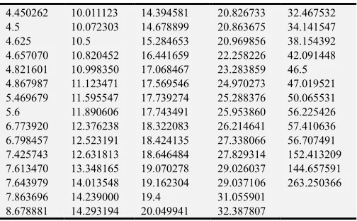
In this study, we are concerned with confidence bounds for the 73 monthly maximum losses during the mentioned from the given 2167 observations, listed in an increasing order.

Table 3. Monthly maximum losses during the mentioned from Danish data for a random sample of n = 73 fire insurance claims.

4.450262 10.011123 14.394581 20.826733 32.467532

4.5 10.072303 14.678899 20.863675 34.141547

4.625 10.5 15.284653 20.969856 38.154392

4.657070 10.820452 16.441659 22.258226 42.091448 4.821601 10.998350 17.068467 23.283859 46.5 4.867987 11.123471 17.569546 24.970273 47.019521 5.469679 11.595547 17.739274 25.288376 50.065531

5.6 11.890606 17.743491 25.953860 56.225426

6.773920 12.376238 18.322083 26.214641 57.410636 6.798457 12.523191 18.424135 27.338066 56.707491 7.425743 12.631813 18.646484 27.829314 152.413209 7.613470 13.348165 19.070278 29.026037 144.657591 7.643979 14.013548 19.162304 29.037106 263.250366

7.863696 14.239000 19.4 31.055901

To begin the search for zeros of

ψ θ

k

( )

we compute the bounds

(

ε θ θ

, _L, _U

)

for k =50.

Then ε=2.817172 10× −9 and other bounds given by 1

-3.018889 10

L

θ

_{= ×} −

, and

θ

_U=3.798662 10× −3. The algorithm will search for two zeros on

[

θ

_L;−

ε

]

and _

ε θ

; _U for

ψ θ

_k

( )

. Using our program yields we found The GPD maximum likelihood estimates for over threshold k >50 monthly maximum losses during the mentioned from the given 73

observations for the Danish data is ˆγ =0.08586831 , ˆ 32.31397400

σ= .

Then, their corresponding 95% confidence intervals is -0.1249036< <γ 0.2966402 and 21.08807 < <

σ

43.53988.

4. Conclusion

Since, the value of γ∈ the shape parameter or extreme value index though it is often referred to as "tail behavior"; in model of extreme values distribution is dominant which are the three standard family see Haan and Ferreira [9] (either Gumbel (γ =0), Fréchet (γ >0), or Weibull (γ <0)). by determining tail behavior. In this paper we introduce a good numerical method with less condition and we avoided many numerical and the negatives of Newton method, which isnot always easy in the practice, and we have reduced time and effort,for maximum likelihood estimate without signs

γ

the shape parameter.

Acknowledgements

Special thanks are due to Dr, Fateh Ben Atia and Dr Djabrane Yahia for his valuable help and the important remarks.

Appendix

The second derivatives of the log-likelihood are computations for

θ

= −

(

γ σ

/

)

by:

( )

(

)

_{( ) ( )}

( )

(

)

( )

(

)

2

2 3

2

1

2

2 2

2

1

2

2

log _{1 1 1}

2 1 1 . 1 2 log 1

1 1

log 1 1 1

1 1 . 2 1 1

1 1

log _{1 1}

1 1

1

k i

i

i i

i k i

i i

i

i

i

C

C

C C

C

C C

C

C

=

=

 

∂   _     _

=   − + +  −  − −

− −

 

∂   _     _

  

∂   _  _     _

=  _ − + _  −  − −  _

− −

∂   _  _     _

∂  

=  − − +

∂ ∂  − 

∑

∑

l

l

l

γ θ

γ θ θ

γ θ

γ γ θ θ

σ θ

γ σ γ θ γ

2

1

1 . 1

1

k

i

i= C

        

  _{  }    _{  − } 

−

 _     _ 

∑

_θ

References

[1] Balkema, August A., and Laurens De Haan., 1974. “Residual life time at great age, The Annals of probability,”. 792-804. [2] Davison, Anthony C., 1984. “Behavior Modelling excesses

over high thresholds, with an application. Statistical extremes and applications,”. Springer Netherlands, 461-482.

[3] Drees, Holger, Ana Ferreira, and Laurens De Haan., 2004. “On maximum likelihood estimation of the extreme value index,” Annals of Applied Probability, 1179-1201.

[4] Embrechts, P., and C. Klüppelberg., T. Mikosch., 1997. “Gas Modelling Extremal Events for Insurance and Finance, Applications of Mathematics-Stochastic Modelling and Applied Probability,”. Springer New York, No. 33.

[5] Fisher, Ronald Aylmer, and Leonard Henry Caleb Tippett., 1928. “Limiting forms of the frequency distribution of the largest or smallest member of a sample,” Mathematical Proceedings of the Cambridge Philosophical Society, Cambridge University Press, Vol. 24. No. 02.

[6] Fachinger, Gnedenko, Boris., 1943. “Sur la distribution limite du terme maximum d'une serie aleatoire Annals of mathematics,”. 423-453.

[7] Grimshaw, Scott D., 1993. “Computing maximum likelihood estimates for the generalized Pareto distribution,”. Technometrics 35.2, 185-191.

[8] Haan, L. DE., 1970. “On regular variation and its application to the weak convergence of sample extremes,”. Mathematical Centre Tracts 32.

[9] Haan, L de. and Ferreira, A., 2006. “Extreme Value Theory: An Introduction,” Springer.

[10] Hosking, Jonathan RM, and James R. Wallis., 1987. “Parameter and quantile estimation for the generalized Pareto distribution,” Technometrics 29.3, 339-349.

[11] Reiss, Rolf-Dieter, Michael Thomas, and R. D. Reiss., 2007. “Statistical analysis of extreme values,” Basel, Birkhüser, Vol. 2.

[12] Smith, Richard L., 1985. “Computing Maximum likelihood estimation in a class of nonregular cases,” Biometrika 72.1, 67-90.

[13] Tanakan, S., 2013. “A New Algorithm of Modified Bisection Method for Nonlinear Equation,” Applied Mathematical Sciences 7.123, 6107-6114.