GPU-accelerated surgery simulation for opening a brain fissure

RESEARCH ARTICLE

GPU-accelerated surgery simulation

for opening a brain fissure

Kazuya Sase

_{, Akira Fukuhara}

_{, Teppei Tsujita}

_{and Atsushi Konno}

Abstract

In neurosurgery, dissection and retraction are basic techniques for approaching the site of pathology. These tech-niques are carefully performed in order to avoid damage to nerve tissues or blood vessels. However, novice surgeons cannot train in such techniques using the haptic cues of existing training systems. This paper proposes a real-time simulation scheme for training in dissection and retraction when opening a brain fissure, which is a procedure for creating a working space before treating an affected area. In this procedure, spatulas are commonly used to perform blunt dissection and brain tissue retraction. In this study, the interaction between spatulas and soft tissues is modeled on the basis of a finite element method (FEM). The deformation of soft tissue is calculated according to a corotational FEM by considering geometrical nonlinearity and element inversion. A fracture is represented by removing tetra-hedrons using a novel mesh modification algorithm in order to retain the manifold property of a tetrahedral mesh. Moreover, most parts of the FEM are implemented on a graphics processing unit (GPU). This paper focuses on parallel algorithms for matrix assembly and matrix rearrangement related to FEM procedures by considering a sparse-matrix storage format. Finally, two simulations are conducted. A blunt dissection simulation is conducted in real time (less than 20 ms for a time step) using a soft-tissue model having 4807 nodes and 19,600 elements. A brain retraction simu-lation is conducted using a brain hemisphere model having 8647 nodes and 32,639 elements with force feedback (less than 80 ms for a time step). These results show that the proposed method is effective in simulating dissection and retraction for opening a brain fissure.

Keywords: Surgery simulation, Finite element method, GPGPU

© 2015 Sase et al. This article is distributed under the terms of the Creative Commons Attribution 4.0 International License (http://creativecommons.org/licenses/by/4.0/), which permits unrestricted use, distribution, and reproduction in any medium, provided you give appropriate credit to the original author(s) and the source, provide a link to the Creative Commons license, and indicate if changes were made.

Background

Virtual reality (VR) surgery simulation is a safe and effi-cient approach to surgical training. In the last two dec-ades, laparoscopic surgery simulators have been widely developed to support efficient training in surgical tech-niques. In contrast, neurosurgery simulators have not been investigated extensively. However, recent years have witnessed some significant advancements in the devel-opment of neurosurgery simulators [1, 2]. Neurosurgery requires surgeons to perform precise operations. Because surgeons rely on haptic cues in various contexts, the physics of soft-tissue deformation should be reliable not only for graphical rendering but also for haptic rendering.

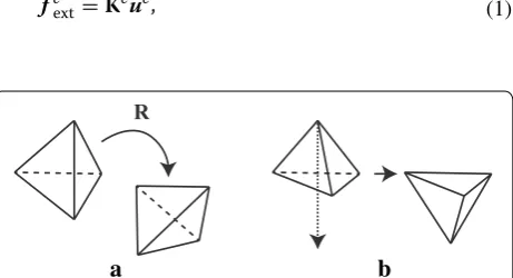
One of the basic procedures in neurosurgery is the opening of a brain fissure, which is necessary to create a working space to access an affected area. Figure 1 shows a schematic of this procedure. In order to approach an affected area located at the bottom of the fissure, sur-geons cut connective tissues such as the arachnoid membrane and arachnoid trabeculae using microscis-sors and push the brain tissues apart to keep the tis-sues open using spatulas  [3]. Aspirators are used to apply tension to the membrane and remove blood. It is known that the position of the spatulas and the pushing force are related to the patient’s prognosis [4]. An early simulator focusing on retraction in neurosurgery was the virtual retractor developed by Koyama et  al.  [5]. It modeled the deformations of intracranial vessels using geometrical theory, but physical consistency was not considered. Hansen et al. developed a real-time simula-tor for brain retraction [6]. They adopted a finite element

Open Access

*Correspondence: [email protected]

1 _{Graduate School of Information Science and Technology, Hokkaido} University, Kita 14 Nishi 9, Kita-ku, Sapporo, Japan

method (FEM) for calculating the deformation of brain tissues and the reaction force. However, the resolution of the mesh was limited to less than a thousand nodes because of its high computational cost. Hasegawa et al. conducted a cerebellar retraction simulation using a high-resolution model [7]. They considered the nonlinear viscoelastic behavior of soft tissues. However, their opti-mization method was inadequate for realizing real-time simulation.

To develop a haptic simulator for opening a brain fis-sure, the following system specifications are required.

• The refresh rate of the physics simulation must be greater than 30 Hz for smooth animation [8].

• The positions of the surgical instruments are input by haptic devices, and the reaction force must be returned immediately. Ideally, the refresh rate of the force feedback should be greater than 1 kHz for interaction with stiff materials [8].

• The number of nodes of target finite element model (brain hemisphere) should be approximately 10,000.

• The ability to perform connective-tissue dissection should be present [8].

• The soft tissues should have physically correct behavior. Brain tissues are known to have complex mechanical properties; for example, white matter is known to have anisotropic visco-hyperelasticity  [9].

Generally, there is a compromise between the precision and the speed for the computation of soft-tissue physics. Therefore, we firstly simplify the mechanical properties of soft tissues and aim to develop a visually acceptable simulator with a refresh rate greater than 30 Hz for the physics simulation.

To fulfill the above-mentioned requirements, we firstly formulated the framework of the interactive

simulation using a linear FEM and combined it with hap-tic devices  [10]. In order to accelerate the calculation, we developed an algorithm for collision detection that is implemented on a graphics processing unit (GPU) [11]. However, the computational speed is not sufficient to run in real-time. In particular, the FEM solver was not opti-mized for calculation on the GPU, and it became the bot-tleneck of the simulation.

In this paper, an efficient implementation of an FEM solver is proposed to simulate the opening of a brain fis-sure. The contributions of this paper are the following:

• A GPU-accelerated method of a corotational linear FEM including a boundary-condition-based collision response is proposed.

• A stabilization algorithm for the fracture simulation based on element removal is incorporated into the proposed GPU-accelerated FEM framework.

In the conventional FEM implementation, the most time-consuming procedures are assembling the stiff-ness matrix and solving linear equations. Moreover, the calculation of the collision response requires additional procedures. In the FEM solver proposed in this paper, the collision response is calculated by applying geometrical boundary conditions. Because conventional FEM solvers do not consider the frequent changes in the geometri-cal boundary conditions, efficient matrix assembly and matrix rearrangement have not attracted much attention. In this paper, the three above-mentioned procedures, i.e., assembling the stiffness matrix, solving linear equations, and rearranging the stiffness matrix, are implemented by considering a sparse-matrix storage format (“ Implemen-tation and GPU parallelization”). All of these algorithms are implemented on a GPU. However, the proposed algo-rithms assume that the mesh topology of analysis area

a

b

c

is constant during a simulation. Therefore, additions of new nodes and changes in the node connectivity are not permitted. In order to realize the ability to dissect under these limitations, we adopt a fracture represen-tation on the basis of the element removal approach. In this approach, fracture behaviors are calculated by inac-tivating the physical contributions of removed elements. However, it has been reported that the dynamic behaviors become unstable, which may lead to diverse the numeri-cal numeri-calculation when the tetrahedral mesh becomes non-manifold because of element removals [12]. To solve the stability problem, we also propose an element removal algorithm to avoid topological singularities (“Modeling of dissection”). The concept of proposed algorithm is active element removal. Its implementation is considerably sim-pler and can be used as alternative to existing methods such as that in [13]. Finally, to evaluate the performance of these implementations, a blunt dissection and brain retraction are simulated, and the results of these simula-tions are presented (“Results”).

Related work Collision response

Recent cutting-edge studies on real-time haptic render-ing for interactrender-ing deformable objects have focused on efficient contact handling including collisions between multiple deformable objects and self-collisions  [14, 15]. They modeled contacts based on Signorini’s law and Cou-lomb’s law, and the linear or nonlinear complementarity problem needs to be solved. Although their algorithms are highly optimized for a GPU, the number of nodes is limited to several thousand for realizing real-time simu-lation because of their high computational costs.

The fastest implementation of collision response is the penalty method [16]. In this method, external forces are applied to contact nodes according to the penetration depth. To compute the magnitude of the external forces, scalar coefficients are required for multiplication with the depth. However, it is difficult to determine the scalar val-ues for obtaining a stable response.

The other approach is the position constraint method. In this method, nodal displacements are directly input according to geometric relations. In an early study on a real-time surgery simulator, Cotin et  al. introduced a position constraint formulation using the Lagrange mul-tiplier method  [17]. Hirota et  al. adopted a boundary-condition-based constraint [18]. Although these method are essentially equivalent and both methods resulting in a large simultaneous linear equations, the method of Hirota et al. has the advantage in the term of the size of the linear equations (see “Collision response of soft tis-sues”). The limitation of this method is that accurate con-tact response subject to Signorini’s law or Coulomb’s law

cannot be computed. However, because the computa-tional cost is lower than that of the accurate methods, the position constraint method can be used for the analysis of a fine detailed mesh.

As mentioned above, the position constraint method based on a boundary condition involves a large number of simultaneous linear equations. Because the linear sys-tem is large and sparse, the sparse matrix format should be adopted for efficient execution of mathematical opera-tions and to reduce memory consumption. However, its GPU-optimized implementations considering the sparse matrix format have not been discussed.

Fracture

In the field of computer graphics, several methods of fracture simulation have been discussed [19–21]. This section describes the details of fracture algorithms devel-oped for real-time applications.

A notable approach is the extended FEM  [22], which allows for representation of any crack without the limita-tions of a mesh topology by adding a shape function to the element displacement field interpolations. Thus, an additional degree of freedom (DOF) is provided to model crack discontinuities.

Mor and Kanade modeled the knife cutting of soft objects [23]. They proposed split patterns in which a tet-rahedron is split into smaller tettet-rahedrons according to the knife path. In this approach, the tetrahedral mesh is explicitly modified by adding new nodes to it.

Delingette et  al. proposed an element removal approach in the early years of surgery simulation stud-ies [24]. Even though this approach suffers from the dis-advantage of a loss of volume, it offers dis-advantages such as a low computational cost and simple implementation. In particular, we focus on the fact that this algorithm does not require the addition of add new nodes. Thus, simula-tions can be performed at the same computational cost throughout. Because real-time characteristics are impor-tant for practical use of the surgery simulator, we adopt this element removal approach.

As shown by Forest, element removal may lead a tet-rahedral mesh to become a nonmanifold geometry [12], which means that the tetrahedral mesh has vertices or edges where the thickness of the volumetric mesh can-not be defined. Vertices and edges are known as singu-lar vertices and singusingu-lar edges, respectively, and such a singularity is known as a topological singularity (Fig. 2). Because the dynamic behavior can be unstable when the FEM mesh becomes a nonmanifold geometry, topologi-cal singularities should be avoided during simulation.

the singular vertices and singular edges by adding cop-ies of such vertices and edges. However, this approach increases the computational cost because the DOFs of the system increase with the addition of nodes. Nakay-ama et al. proposed a delay algorithm that suspends the removal of elements that cause topological singulari-ties [13]. However, the delay algorithm does not correctly simulate actual fracture phenomena. In the actual case, the stress will be concentrated at a singular vertex and singular edge. Thus, the two elements connected by a sin-gular vertex or sinsin-gular edge will be disconnected. There-fore, such elements should be removed immediately.

Finite element model of the brain Corotational FEM

The corotational formulation is an approximate approach that considers the geometrical nonlinearity for small strain deformations. This formulation evaluates element strains with respect to the rotated element coordinates, which are referred to as corotational coordinates (see Fig. 3a). A corotational coordinate is a coordinate that is rotated using the rotation component of the current deformed configuration. A corotational FEM is a reason-able choice for achieving a trade-off between precision and computational cost [25]. In general, the element stiff-ness equation is defined as

(1)

fe_ext=Ke_ue_,

where fe_ext and ue are the nodal force and displacement vectors of an element, respectively. The element dis-placement vector is defined as ue=xe−xe₀, where xe and xe₀ are the displaced and initial nodal position vec-tors of the element, respectively. If the rotation of the element coordinates is represented by a rotation matrix R_∈R3×3, the displaced position and force vectors are transformed by R and the element stiffness equation becomes

where Ke

0 is the element stiffness matrix of a linear FEM and Re_{blockdiag [}R_,R_,R_,R_]. The above equation is rewritten as

where

fe₀ is known as the force offset vector.

R is calculated by singular value decomposition (SVD) of deformation gradient. The details are described in “Appendix A: Rotation of a deformed tetrahedron”.

Matrix/vector assembly After Ke and _fe

0 are obtained, the global stiffness matrix K_∈R3Nnode×3Nnode and global force offset vector

f₀∈R3Nnode, where _N

node is the number of nodes, are

calculated by gathering all element contributions using connectivity information. This procedure is known as matrix/vector assembly, and it is expressed as

(2) ReT_fe_ext=K₀eReT_xe_−xe_0,

(3) fe_ext=Ke_xe−fe₀,

(4) Ke=ReKe₀ReT_,

(5) fe₀=ReKe_0xe₀;

(6) K=

e

LeTKeLe_,

(7)

f₀=

e LeT_fe_0,

Fig. 2 Topological singularity

a

b

where Le∈R12×3Nnode is the gather matrix, which

gath-ers element nodal data from global vectors. Le is a Boolean matrix, which consists of zeros and ones. Note that Eqs.  (6) and (7) are just mathematical formula-tions; the actual assembly process is implemented in a more efficient manner. The efficient implementations are described in “Efficient matrix/vector assembly in a sparse storage format”.

The global stiffness equation is written as

where f_ext and x are the global external force vector and global position vector, respectively. For simplicity, this equation can be written by analogy to the global stiffness equation of a linear FEM as

where f =f_ext−f₀.

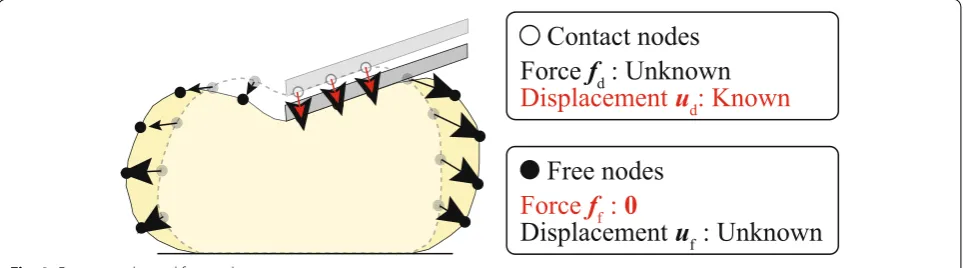
Collision response of soft tissues

When a surgical instrument contacts with the brain model, it is assumed that the contact nodes move together with the instrument (Fig. 4). Hence, the dis-placements of the contact nodes are known, but their contact forces are unknown. In contrast, the displace-ments of free nodes and internal nodes are unknown, but their external forces are known (they are zeros). There-fore, the nodes are rearranged into displacement-known nodes and force-known nodes, and Eq. (9) can be modi-fied by rearranging the matrix and vectors as follows [18]:

where the suffixes f and d denote the components of the force-known and displacement-known nodes, respec-tively. As shown in Fig. 4, the contact nodes are geomet-rically constrained on the surface of a rigid body (surgical instrument). Hence, the displacements of the contact nodes are known, whereas the forces are unknown. In (8) f_ext=K_x−f₀,

(9) f =K_x,

(10)

f_f f_d

=

K_ff K_fd K_df K_dd

xf xd

,

contrast, the forces generated at unconstrained nodes are zero under the stationary condition, whereas the displacements are unknown. In Eq.  (10), f_d and x_f are unknown, and x_f is obtained by solving the following lin-ear equation:

After x_f is obtained, the other unknown value f_d is cal-culated as

Although only the formulation of the static FEM is described above, the adoption of the formulation of the dynamic FEM with implicit time integration introduces a mathematically similar equation to the formulation of static FEM. The details of the formulation of the dynamic FEM are presented in “Appendix B: Formulation of a dynamic FEM”.

Implementation and GPU parallelization

This section describes the implementation of the FEM. To measure the computational time, we used a CIARA KRONOS S810R workstation, which employs an Intel Core i7-3960X (six cores, overclocked to 4.5 GHz) CPU with 64  GB of RAM and two GPUs, an NVIDIA K20c (2,496 CUDA cores) for general-purpose computing and an NVIDIA Quadro K5000 (1536 CUDA cores) for graphics processing. Parallel processing is implemented using OpenMP for multithread computing on a multi-core CPU and NVIDIA CUDA for general-purpose com-puting on GPUs (GPGPU).

Simulation procedures

The flowchart of our simulation scheme is shown in Fig. 5. Before the real-time simulation loop, the element stiffness matrices of the linear elasticity Ke

0 and the reduc-tion lists described in “Efficient matrix/vector assembly in a sparse storage format” are calculated. The real-time simulation procedures are as follows.

(11) K_ffxf =f_f −K_fdxd.

(12) f_d=K_dfxf +K_ddxd.

Calculation of element data: Re, Ke, and _fe₀ are calcu-lated. The details of these parallel implementations are described in “Calculation of element data”.

Matrix/vector assembly: K and _f0 are assembled. The details of the parallelization of the assembly are described in “Efficient matrix/vector assembly in a sparse storage format”.

Collision detection: Collision detection between a deformable object (brain) and rigid objects (brain spatulas) is executed. The contact nodes of the deformable object and the corresponding forced dis-placements are determined. The discrete collision detection approach reported in  [11] is adopted. This method can deal with collisions between a nonconvex deformable object and a rigid object.

Application of boundary condition: On the basis of collision detection, a boundary condition is set. As mentioned in “Collision response of soft tissues”, a large sparse matrix is rearranged according to the boundary condition. The implementation details are described in “Matrix rearrangement”.

Calculation of the deformation and external forces: The calculation of the deformation is a problem involv-ing a system of linear equations. The linear equations are solved by the conjugate gradient method. Sparse-matrix dense-vector multiplications are implemented by the sparse-matrix library CUSPARSE provided by NVIDIA Corp.

Calculation of element data

An element stiffness matrix Ke is calculated using Eq. (4). It is assumed that the materials are isotropic; hence, Ke is a symmetric matrix. Therefore, it is sufficient to store the elements of the upper triangular matrix of Ke. Further,

fe₀ is calculated in the same way as Ke (Eq. 5). Finally, all Ke (K1, K2_,. . .,KNelem) and _fe

0 (f10, f20,. . .,f

Nelem

0 ), where Nelem is the number of tetrahedral elements, are

serial-ized and stored in the arrays valuesKe and valuesF0e, respectively. These procedures are implemented in paral-lel using one thread per element.

Efficient matrix/vector assembly in a sparse storage format In the matrix/vector assembly procedure, the element stiffness matrices are assembled into the global stiffness matrix, as described in Eq.  (6), and the element force offset vectors are assembled into the global force off-set vector, as described in Eq. (7). First, the implemen-tation of global stiffness matrix assembly is described, and then, that of global force offset vector assembly is described.

In most FEM problems, the global stiffness matrix is a large sparse matrix that is stored in a sparse-matrix stor-age format to reduce memory consumption. In this work, the global stiffness matrix is stored using the coordinate list (COO) sparse storage format during matrix assem-bly. This is because of the requirement of matrix rear-rangement described in “Matrix rearrangement”. The COO consists of three arrays: values, rowIndices, and

columnIndices. In the COO format, only the nonzero

ele-ments of a sparse matrix are stored in the array values. The row and column indices of the nonzero elements are stored in the arrays rowIndices and columnIndices,

respectively. These arrays are stored in row-major order. For example, the matrix

is stored as the following three arrays.

In the remainder of this section, values, rowIndices, and

colmunIndices represent the arrays of K in the COO format.

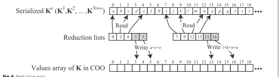
In order to implement a fast matrix assembly algo-rithm, we adopted the reduction list approach proposed in [26]. When the mesh topology does not change during simulation, rowIndices and columnIndices are constant matrices. Hence, only values should be updated at every time step. Matrix assembly involves a number of inde-pendent summations expressed as





a b 0

0 c 0

0 0 d





values= [a,b,c,d] rowIndices= [0, 0, 1, 2] columnIndices= [0, 1, 1, 2]

(13)

values(i)= Nsrc,i

j=1

valuesKe(srcIndicesi(j)),

where srcIndicesi is an array that stores the source indi-ces pointing to the components of valuesKe for the sum-mation of the i-th component of values, and Nsrc,i is the number of components of srcIndicesi. The components of srcIndices are determined by the connectivity of a tet-rahedral mesh. A reduction list stores the source indices and a negative-signed destination index as

As shown in Eq. 14, a reduction list has one destination index in general. On the other hand, because we assume that the material is isotropic and K is a symmetric matrix, the reduction list can store two destination indices as

where lower(i) is an index pointing to the lower

compo-nent of values(i). An example of reduction-array-based

summation is shown in Fig. 6. For a symmetric matrix, there is a storage format that stores only upper or lower triangular entries as in the case of Ke_{. However, the} adoption of such a storage format for K requires special treatment in the subsequent procedures, which might degrade the maintainability because of its complexity. Thus, all the nonzero components of K are stored using this reduction procedure. This approach avoids atomic operation because the output memories are independent of each other as in the case of the general reduction list approach.

The assembly of f₀ is implemented in a similar man-ner. After the calculation of Re_{, all values of f}e

0 are stored as an array. The reduction list for the assembly of f₀ is constructed in advance. The reduction is performed in a thread per component of f₀, which allows for the calcu-lation of f₀ without atomic operation. This reduction is independent of the assembly of K. Therefore, assemblies of K and _f

0 are performed concurrently, e.g., on two GPUs.

(14)

reductionListi= [srcIndices(1),srcIndices(2),. . .,

srcIndices(Nsrc,i),−i].

(15)

reductionListi= [srcIndices(1),srcIndices(2),. . .,

srcIndices(Nsrc,i),−i,−lower(i)],

Matrix rearrangement

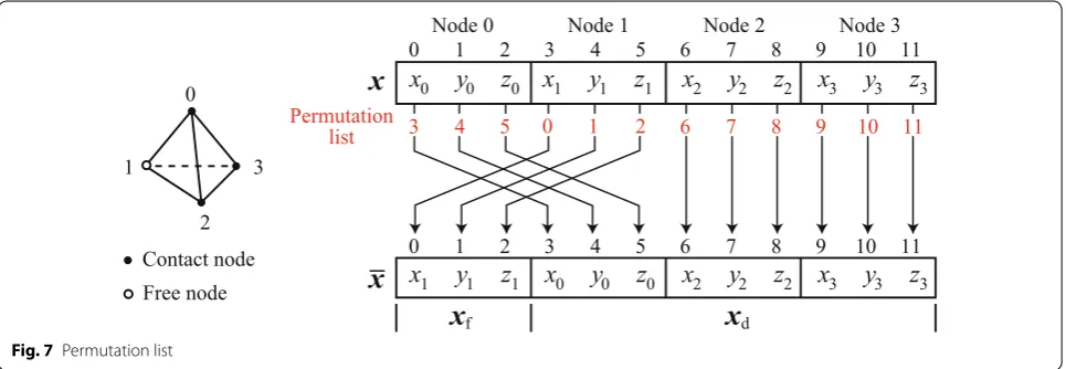
As described in “Collision response of soft tissues”, col-lisions are represented by geometrical boundary con-ditions and the global stiffness matrix is rearranged by considering the boundary conditions. This rearrange-ment procedure involves permutation and separation processes.

Permutation is performed by referring to a permuta-tion list that includes the source index i and destina-tion index list(i). The list is constructed according to the

boundary conditions. Figure 7 shows an example of per-mutation in the case of one tetrahedron, in which nodes 0, 2, and 3 are constrained. The permutation procedure accumulates the variables of the contact nodes at the head of the array and those of the free nodes at the bot-tom. Permutation using a permutation list is represented as m′(list(i),list(j))=m(i,j), where m and m′ represent the source matrix and permutated matrix, respectively, and m(i, j) denotes the i, j component of matrix m. If a matrix is stored as a dense matrix, permutation is per-formed by simply copying the source components to the destinations. However, if the matrix is stored in a sparse storage format, the implementation of permutation dif-fers according to the storage format.

In this work, the global stiffness matrix is stored in the COO format, as mentioned in “Efficient matrix/vector assembly in a sparse storage format”. In the COO format, permutation is easily and efficiently performed as

These operations do not conflict with each other, and all permutations are performed in parallel. Other sparse storage formats such as compressed sparse row (CSR) are also widely used. The CSR format can be constructed by compressing rowIndices used in the COO format. This approach can further reduce the memory consumption compared to the COO format, and it is suitable for par-allelizing matrix–vector multiplication. However, the

(16)

rowIndices(i)=list(rowIndices(i)), columnIndices(i)=list(columnIndices(i)).

implementation of permutation is not easier than that of the COO format. Although it can be realized using the permutation matrix P as M′₌PTMP, this

implementa-tion is not efficient because the memory traffic increases and additional arithmetic operations are required com-pared to the COO format. Therefore, the COO format was selected as the sparse storage format in this work.

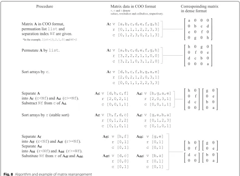
Sorting should be performed to maintain the row and column index arrays in ascending order; however, the sorting process can be combined with a separation pro-cess. An overview of the entire procedure including per-mutation and separation is shown in Fig. 8 by taking a matrix A as an example. After Eq. (16) is executed, three arrays are sorted by columnIndices. Next, A is separated along its columns into A_f and A_d. When the separation index is Nf, entries whose column index is less than Nf are copied to A_f. The other entries are copied to A_d. In order to fix columnIndices to zero-base indices, Nf is sub-tracted from all of the components of columnIndices in A_d. Subsequently, three arrays, namely values,

rowInd-ices, and columnIndices of A_f and A_d, are sorted by their

rowIndices. Note that this sorting must be stable, which means that the original order is maintained when the compared values are equal to each other. This is because the ascending order of columnIndices might be disturbed if the sorting is not stable. After sorting, A_f and A_d are separated along their rows into A_ff, A_df, A_fd, and A_dd . Subtraction of rowIndices of A_df and A_dd is performed for the same reason as that for A_d. Finally, the separated matrices are obtained in the COO format.

These procedures require sorting of large arrays, which is computationally expensive. In order to accelerate the sorting process, they are implemented on a GPU using the NVIDIA CUDA thrust library.

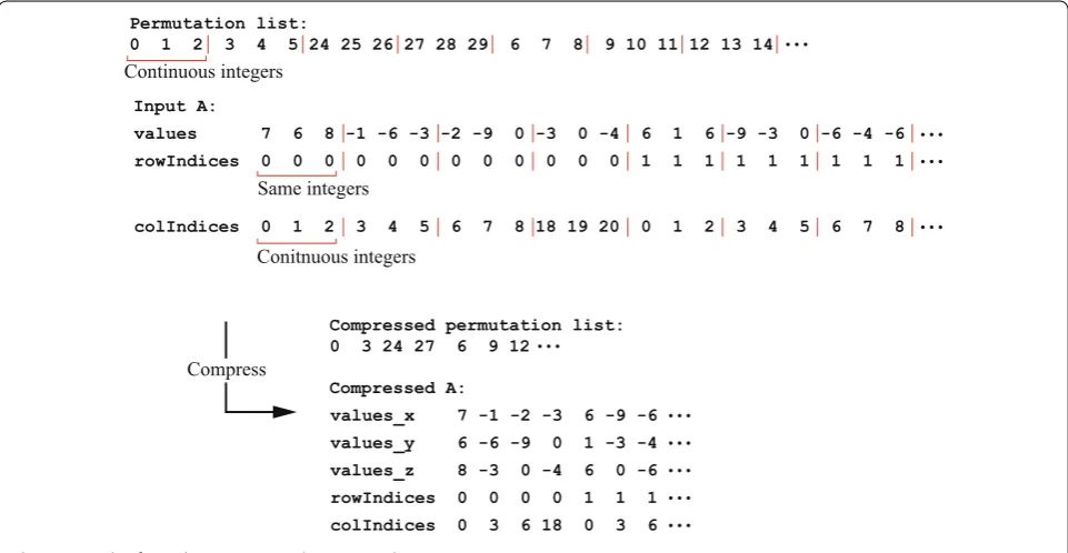
For further optimization, the permutation list and the arrays (values, rowIndices, columnIndices) of A can be

compressed by considering the series order of the arrays of A. An example of the compression is shown in Fig. 9. Because three variables of each node are relocated together, the permutation list becomes a combination of three con-secutive integers. Moreover, rowIndices and columnIndices

consist of a combination of the same three integers, i.e., (0, 0, 0), and a combination of three consecutive integers, i.e., (0, 1, 2), respectively. Hence, sorting is performed accord-ing to these three-integer blocks. In order to sort per block,

values is separated into three arrays, values_x, values_y, and values_z. Next, the permutation list, rowIndices, and

columnIndices are compressed by storing only the first ele-ment of the consecutive-integer blocks. This compression reduces the size of the arrays to a third of their original size and the computational cost of sorting decreases. After A_ff, A_fd, A_df, and A_dd are obtained, the compressed arrays are extracted in the original COO format.

Modeling of dissection

Topological‑singularity avoidance algorithm for element removal

This section describes a simple and efficient topological-singularity avoidance algorithm for element removal. The basic concept of the approach is active element removal. Although the volume decreases as elements are removed, the approach is fast and easy to implement. The flow of the algorithm is summarized as follows.

1. Fracture detection Determine the tetrahedrons to be removed on the basis of a specified fracture criterion and list them in a set Trm.

2. Singularity verification Check whether the verti-ces and edges that belong to Trm are singular after removing the tetrahedrons listed in Trm.

3. Detection of additional tetrahedrons to be removed If any vertices or edges are predicted to be singular, the

tetrahedrons that include the predicted singular ver-tices or edges are added to Trm.

4. Repeat Singularity verification and Detection of addi-tional tetrahedrons to be removed until Trm becomes empty.

The maximum principal stress is selected as the cri-terion to determine the tetrahedrons to be removed. If the absolute value of the maximum principal stress of an element exceeds a previously specified threshold, the element is listed in Trm, the set of tetrahedrons to be removed. Hence, the removal criterion is defined as

where σ_i(i=1, 2, 3) is the maximum principal stress of

a tetrahedron, which is obtained as the eigenvalue of the stress tensor Se, and σ_max is the previously specified

stress threshold. Note that we use a constant strain ele-ment; and thus, Se becomes constant on an element. In the corotational FEM, Se is calculated by considering the element rotation as Se₌DeBe

Re_xe_−xe

0

, where De and (17)

max(|σ1|,|σ2|,|σ3|) > σmax,

Be are the strain–stress matrix and displacement–strain

matrix, respectively.

In the singularity detection phase, the sets of vertices Vrm and edges Erm are constructed from the

tetrahe-drons listed in Trm. Each vertex v∈Vrm and edge e∈Erm is checked for a singularity. The algorithm of singularity detection of vertex v is summarized as follows. An exam-ple is shown in Fig. 10a.

1. Extract Tv, a set of tetrahedrons, that includes v as a vertex.

2. Select an arbitrary tetrahedron t₀v∈Tv.

3. Construct T_edgev , a set of tetrahedrons, that shares at least one edge with t₀v.

4. Select a tetrahedron t_xv∈T_edgev and search for an

edge-sharing tetrahedron as described above in steps 2 and 3. Add the new edge-sharing tetrahedron to T_edgev and repeat until no entry is found.

5. If n(Tv)�=n(T_edgev ), v is a singular vertex, where n(·)

denotes the number of tetrahedrons.

The algorithm for singular edge detection is similar to that for singular vertex detection, as it is summarized as follows. An example is shown in Fig. 10b.

1. Extract Te, a set of tetrahedrons, that include e as an

edge.

2. Select an arbitrary tetrahedron t₀e∈Te.

3. Construct T_edgee , a set of tetrahedrons, that shares at

least one edge with t₀e except edge e.

4. Select a tetrahedron t_xe∈T_edgee and search for an

edge-sharing tetrahedron as described above in steps 2 and 3. Add the new edge-sharing tetrahedron to

T_edgee and repeat until no entry is found.

5. If n(Te)�=n(T_edgee ), e is a singular edge.

The detection of additional tetrahedrons to be removed phase determines a set of additional tetrahedrons to be removed, Tadd, in order to avoid a topological singu-larity. When a singular vertex v is detected, T_edgev and

ˆ

T_edgev

=Tv∩ ¯T_edgev

are defined. In order to prevent the loss of volume as much as possible, the number of tetra-hedrons to be removed should be minimized. Therefore, the smaller set between T_edgev and Tˆ_edgev is selected as Tadd by comparing n(T_edgev ) and n(Tˆ_edgev ). For the same

rea-son, when a singular edge e is detected, the smaller set between T_edgee and Tˆ_edgee =Te∩ ¯T_edgee is selected as Tadd. After Tadd is determined, it is added to Trm as mentioned at the beginning of this section.

Examples of fracture simulations are shown in Fig. 11. In the simulation without topological-singularity avoid-ance (Fig. 11b), tetrahedrons connected with only a sin-gular vertex or edge exhibit unstable deformation. On the other hand, in the simulation with topological-singularity avoidance (Fig. 11a), the risk of instability is eliminated, and the simulation continues in any fracture situation.

Implementation

The calculation of the maximum principal stress on each element is computed in parallel by the GPU. To calcu-late the eigenvalues of the stress tensor, the Jacobi eigen-value algorithm is adopted. The singularity avoidance algorithm is implemented on a six-core CPU because it requires numerous conditional branchings and compli-cated data structures for the mesh topology. However, it is not a time-consuming procedure and is rapidly com-puted, even on a CPU.

Results

Performance evaluation of GPU implementations

We compare three implementations of matrix/vector assembly and matrix rearrangement procedures: (1) a CPU with no parallelization, (2) a six-core CPU with multithread parallelization, and (3) a GPU implementa-tion. Cube-shaped models discretized by various num-bers of tetrahedrons were used for the comparison. The surface nodes of the two opposite sides of the cube are

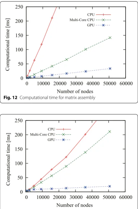
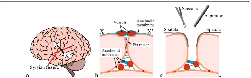
constrained. The execution times of the three differ-ent implemdiffer-entations of the matrix/vector assembly and matrix rearrangement procedures are plotted in Figs. 12 and 13, respectively.

Blunt dissection simulation

Blunt dissection is an operation for separating tissues without cutting. It is generally performed along fissures by breaking connective tissues. In neurosurgery, sur-geons perform cutting operations using scissors or blunt dissection depending on the context of the surgery.

An FE model of a cube with a fissure (4807 nodes and 19,600 tetrahedrons) was used in the simulation. It was assumed that the fissure was filled with connective tis-sues, the Young’s modulus and Poisson’s ratio of which

were 100 and 0.4 Pa, respectively. The Young’s modulus and Poisson’s ratio of the main body were assumed to be 1000 and 0.4 Pa, respectively. The fracture threshold stresses were set to the same values as their Young’s mod-uli. Note that these mechanical parameters are deter-mined to distinguish the relative stiffness of the materials and not validated by experiments. Initially, the tips of two spatulas were inserted into the fissure, and then they were opened to dissect the connective tissues at a velocity of 5.0 mm/s. In order to compare different tions, this simulation was executed by each implementa-tion with a constant time step of 20 ms.

The simulation was conducted without oscillation or divergence. Figure 14a, b show the snapshots and its principal stress visualizations during the simula-tion. Figures 15 and 16 show the calculation time and the number of removed elements at each time step. An additional movie file shows the following simulations in greater detail (see Additional file 1).

Brain retraction simulation

Brain retraction is an operation performed by push-ing soft tissues to create a workpush-ing space. One of the important brain fissures, which are frequently performed retractions, is the the Sylvian fissure. The Sylvian fissure is filled with the arachnoid mater, which needs to be dis-sected by surgeons. This section shows the result of a brain retraction simulation conducted in real-time by user input using a Sensable Phantom Omni haptic device. The reaction force to the user-controlled instruments was fed back through the haptic device. The simulation was conducted under the assumption that the arachnoid mater was dissected beforehand. The task objective given to the user is to retract the brain tissues and expose the brain tumor existing at the bottom of the Sylvian fissure.

(a)

(b)

Fig. 10 Example of topological singularity detection. a Singular vertex detection. b Singular edge detection

A brain hemisphere mesh model (8647 nodes, 32,639 ele-ments) was used in this simulation. This model was con-structed by scanning an anatomical model of the human brain, Brain Model C20 (3B Scientific GmbH), and modi-fying it using 3D modeling software. The bottom nodes of the hemisphere mesh model were fixed; hence, the dis-placements of the bottom nodes were always set to zero.

Figure 17 shows the overview of the simulation. An operator moves a pointer displayed on the monitor by controlling a haptic device. Using the pointer, the oper-ator can pick up and control the spatulas in the virtual space. Collision detection is performed between each spatula and the brain model. The reaction force applied to the spatula from the virtual brain is fed back by the haptic device. As seen in Fig. 17, the Sylvian fissure was opened by two spatulas and the tumor was exposed. Figure 18 shows the calculation time of the time steps. The calculation times for assembling a matrix, rearrang-ing a matrix, and solvrearrang-ing a linear system of equations are plotted. In this simulation, a stress analysis and the frac-ture procedure were not performed. Figure 19 shows the

time history of the raw and filtered reference forces by a first-order low-pass filter (cut-off frequency 1.0 Hz). An additional movie file shows the following simulations in greater detail (see Additional file 1).

Discussions

Figures 12 and 13 show that the GPU implementations had the highest speed among the three implementations in both evaluations. In the comparison of the matrix/ vector assembly, for the model with 15,625 nodes and 69,120 elements, the GPU implementation (10.7  ms) was 19.7 times faster than the single-CPU implemen-tation (210.9  ms) and 3.9 times faster than the six-core CPU implementation (41.9  ms). In the comparison of the matrix rearrangement, for the same model, the GPU implementation (11.0 ms) was 7.1 times faster than the single-CPU implementation (78.4  ms) and 5.1 times faster than the six-core CPU implementation (56.3 ms).

The results of the blunt dissection simulation show that the combination of our GPU implementation and the fracture algorithm worked as expected. As seen in Fig. 14b, the connective tissue was easily deformed and removed owing to the stress concentration because it was specified to be softer than the main body. In Fig. 15, the calculation time jitter is shown. One of the causes is the difference in the convergence times of the conjugate gra-dient method. Another cause is the change in the bound-ary condition. When the boundbound-ary condition changed, the matrix rearrangement procedure is executed and takes additional calculation time. The average calcula-tion times of the three implementacalcula-tions, a CPU with no parallelization, a six-core CPU with multithreaded paral-lelization, and a GPU implementation, were 103, 41, and 17 ms, respectively. The speed-up of the GPU versus the CPU was 6.1. Only the GPU realized smooth animation with a refresh rate greater than 30 Hz. As seen in Fig. 16, the fracture started at step 25, and the peak number of removed elements was 33 at step 60. It is shown that the number of removed elements did not affect the calcula-tion time. This result shows that this approach is prefer-able for surgery simulation because the simulation can be continued at the same refresh rate throughout.

On the other hand, the results of the brain retraction simulation show that our implementation could not achieve the target calculation speed. The range of calcu-lation time for a time step was 40–80  ms. This refresh rate is not sufficient for visually acceptable animations and reaction-force rendering. The reference force was discontinuous, and the force display could oscillate if we did not apply the low-pass filter. Although the low-pass filter reduced the discontinuous force feedback, this is not a fundamental solution for displaying realistic reac-tion forces. From these results, further accelerareac-tion is

Fig. 12 Computational time for matrix assembly

needed to achieve stable and visually acceptable simu-lation. Moreover, the development of a method for dis-playing smooth and stable forces is a topic for future study.

Conclusion

In this paper, a real-time simulation scheme for soft-tissue deformation and fracture for brain retraction is proposed. GPU implementations for matrix/vec-tor assembly and a matrix rearrangement procedure for accelerating a corotational FEM including bound-ary-condition-based collision response are proposed.

A simple mesh modification method considering the avoidance of topological singularities is developed and combined with the proposed GPU-accelerated FEM framework. Finally, blunt dissection and brain retraction simulations are performed using the proposed imple-mentation. Both simulations can be conducted in real time. Although the proposed method could not achieve a visually acceptable update rate for the brain retraction simulation using our target brain hemisphere model, it performs faster than the CPU implementations.

In this study, viscoelasticity and material nonlineari-ties were not considered. In order to obtain more realistic

Fig. 14 Results of the blunt dissection simulation. a Snapshots. b Stress visualization. The colors of the tetrahedrons represent the regularized absolute values of the maximum principal stress max(|σ1|,|σ2|,|σ3|)/σmax, where σ_i(i=1, 2, 3) and σmax are the principal stresses and the fracture

threshold stress, respectively

material behavior, we plan to integrate material proper-ties more precisely in our future implementation.

Authors’ contributions

AK led and directed the project. AK and TT showed the need for a fast and stable calculation method of deformation and fracture of soft tissues for neurosurgery. KS proposed the algorithms implemented them on a GPU, and drafted the manuscript. TT, AF, and AK participated in the discussion on the optimization of the algorithms. Furthermore, TT implemented the base Additional file

Additional file 1. Blunt dissection simulation and brain retraction simula-tion using the proposed method.

simulation framework, and AF implemented the collision detection procedure. All authors read and approved the final manuscript.

Author details

1 _{Graduate School of Information Science and Technology, Hokkaido} Univer-sity, Kita 14 Nishi 9, Kita-ku, Sapporo, Japan. 2 _{Graduate School of Engineering,} Tohoku University, 2-1-1 Katahira, Aoba-ku, Sendai, Japan. 3 _{Graduate School} of Science and Engineering, National Defense Academy, 1-10-20 Hashirimizu, Yokosuka, Japan.

Acknowledgements

This work was supported by JSPS through the Funding Program for Next Generation World-Leading Researchers (LR003), the Grant-in-Aid for Scientific Research (A) (15H01707), the Grant-in-Aid for Challenging Exploratory Research (24650288), and the Grant-in-Aid for JSPS Fellows (15J01452).

Fig. 17 Brain retraction simulation

Fig. 18 Computational time of the brain retraction simulation

Competing interests

The authors declare that they have no competing interests.

Appendix 1: Rotation of a deformed tetrahedron

A rotation matrix of a tetrahedron element is obtained by SVD of the deformation gradient tensor F [27]. This

formulation is stable even if the elements are inverted (see Fig. 3b). In the case of the first-order tetrahedral ele-ment, F transforms an edge vector of the initial shape dmj into an edge vector of the deformed shape dsj as

dsj =Fdmj(j=1, 2, 3). From this equation, F is

cal-culated as F=D_sD−_m1, where D_s=[ds1ds2ds3] and D_m=[dm1dm2dm3]. F can be represented as

where U and V are orthogonal matrices, and is a diago-nal matrix. The rotation matrix is calculated as

where Cdiag

1, 1, det(UVT) [28].

To obtain the rotation matrices of the tetrahedral ele-ments, SVD of a large number of 3×3 matrices described

in Eq.  (18) must be performed. However, most existing parallel implementations of SVD are specialized for large matrices [29]. For SVD of a large number of small matrices, Bedkowski et al. introduced an algorithm for three-dimen-sional reconstruction using mobile robots [30]. In the pre-sent work, the algorithm introduced by Bedkowski et al. is modified. The modified algorithm is summarized as follows:

1. Diagonalize FTF by the Jacobi eigenvalue algorithm

as FTF₌VTSV, where V is an orthogonal matrix,

and S is a diagonal matrix whose elements are the eigenvalues of FTF.

2. Construct a matrix whose diagonal elements are the singular values of FTF. The singular values are

obtained by calculating the square root of each diag-onal element of S.

3. Calculate U₌FV−1.

4. U and V are used in Eq. (19).

In this algorithm, the eigenvalue approach is different from that of Bedkowski et al. They calculated the eigen-values by obtaining the roots of a cubic polynomial. On the other hand, we adopted the Jacobi eigenvalue algo-rithm to simplify the implementation.

Appendix 2: Formulation of a dynamic FEM

The equation of motion for a deformable object is written as

where M and C are a mass matrix and a damping matrix, respectively. M is a diagonal matrix determined by

(18)

F₌UVT_,

(19) R₌UCVT_,

(20)

M_x¨+C_x˙+(K_x+f0)=fext,

gathering the equivalent masses of all nodes from the node-share tetrahedrons: mi=TimTi/4, where mi is the equivalent mass of node i, Ti is a tetrahedron that shares node i, and mTi is the mass of Ti. In general, C is

determined on the basis of the material constitutive law. However, for simplicity, Rayleigh damping is adopted in this study:

where α and β are scalar values representing the damping effect, which are selected heuristically for stabilizing the simulation.

Eq. (20) can be written in the same form as the linear FEM form as

by defining a vector f =f_ext−f₀. When we substitute v for x˙, the time derivatives of the variables are defined as

In order to avoid numerical instability in the dynamic simulation, we adopt implicit time integration because it has unconditionally stable characteristics. Implicit time integration is formulated as

By substituting Eqs. (21) and (25) into Eq. (26), vi+1 can be obtained by solving the following equation:

As discussed in “Collision response of soft tissues”, the contact nodes move together with the rigid body; hence, x_d and v_d are known, whereas f_d is unknown. The forces applied to the unconstrained nodes are zero, i.e., f_f =0. Therefore, Eq. (27) can be rewritten as

where

(21) C=αM+βK_,

(22)

Mx¨+Cx˙+K_x=f

(23)

˙

x=v,

(24)

Mv˙= −C_v−K_x+f.

(25) xi+1=xi+tvi+1,

(26)

M_vi+1=M_vi+t−C_vi+1−K_xi+1+fi+1

.

(27)

(1₊α�t₎M₊

β�t₊�t2

K

vi+1

=M_vi+�t₋K_xi+fi+1

.

(28)

(1_+α�t₎M¯ _+β�t_+�t2K¯_v¯i+1

= ¯Mv¯i+�t

− ¯Kx¯i+ ¯fi+1

,

¯

M₌

M_f 0

0 M_d

, K¯ ₌

K_ff K_fd K_df K_dd

,

¯ v=

vfvd

, x¯ =

xf xd

, f¯=

f_f f_d

Eq. (28) is rewritten as

Received: 23 May 2015 Accepted: 13 December 2015

References

1. Delorme S, Laroche D, DiRaddo R, Del Maestro RF (2012) Neurotouch: a physics-based virtual simulator for cranial microneurosurgery training. Neurosurgery 71:32–42

2. Banerjee PP, Luciano CJ, Lemole GM, Charbel FT, Oh MY (2007) Accuracy of ventriculostomy catheter placement using a head- and hand-tracked high-resolution virtual reality simulator with haptic feedback. J Neurosurg 107:515–521

3. Yasargil MG (1995) Microneurosurgery. Thieme

4. Zhong J, Dujovny M, Perlin AR, Perez-Arjona E, Park HK, Diaz FG (2003) Brain retraction injury. Neurol Res 25:831–838

5. Koyama T, Okudera H, Kobayashi S (1999) Computer-generated surgical simulation of morphological changes in microstructures: concepts of “virtual retractor”. J Neurosurg 90(4):780–785

6. Hansen KV, Brix L, Pedersen CF, Haase JP, Larsen OV (2004) Modelling of inter-action between a spatula and a human brain. Med Image Anal 8(1):23–33 7. Hasegawa Y, Adachi K, Azuma Y, Fujita A, Kohmura E, Kanki H (2010) A

study on cerebellar retraction simulation for developing neurosurgical training system. J Jpn Soc Comput Aided Surg 12(4):533–543 8. Spicer MA, van Velsen M, Caffrey JP, Apuzzo MLJ (2004) Virtual reality

neurosurgery: a simulator blueprint. Neurosurgery 54:783–798 9. Sahoo D, Deck C, Willinger R (2014) Development and validation of an

advanced anisotropic visco-hyperelastic human brain FE model. J Mech Behav Biomed Mater 33(1):24–42

10. Konno A, Nakayama M, Chen XS, Fukuhara A, Sase K, Tsujita T, Abiko S (2013) Development of a brain surgery simulator. In: Proceedings of the International Symposium on Interdisciplinary Research and Education on Medical Device Developments, pp 29–32

11. Fukuhara A, Tsujita T, Sase K, Konno A, Jiang X, Abiko S, Uchiyama M (2014) Proposition and evaluation of a collision detection method for real time surgery simulation of opening a brain fissure. ROBOMECH J 1(1):6 12. Forest C, Delingette H, Ayache N (2005) Removing tetrahedra from

mani-fold tetrahedralisation: application to real-time surgical simulation. Med Image Anal 9(2):113–122

13. Nakayama M, Abiko S, Jiang X, Konno A, Uchiyama M (2011) Stable soft-tissue fracture simulation for surgery simulator. J Robot Mechatron 23(4):589–597

(29)

A_ff A_fd A_df A_dd

vi_f+1 vi_d+1

=

bi_f+1 bi_d+1

.

14. Courtecuisse H, Jung H, Allard J, Duriez C, Lee DY, Cotin S (2010) Gpu-based real-time soft tissue deformation with cutting and haptic feedback. Prog Biophys Mol Biol 103:159–168

15. Courtecuisse H, Allard J, Kerfriden P, Bordas SPA, Cotin S, Duriez C (2014) Real-time simulation of contact and cutting of heterogeneous soft-tissues. Med Image Anal 18(2):394–410

16. Galoppo N, Tekin S, Otaduy MA, Gross M, Lin MC (2007) Interactive haptic rendering of high-resolution deformable objects. In: Proceedings of the 2nd International Conference on Virtual Reality, pp 215–233

17. Cotin S, Delingette H, Ayache N (1999) Real-time elastic deformations of soft tissues for surgery simulation. IEEE Trans Visual Comput Graph 5(1):62–73

18. Hirota K, Kaneko T (2001) Haptic representation of elastic objects. Pres-ence Teleoper Virtual Environ 10(5):525–536

19. O’Brien JF, Bargteil AW, Hodgins JK (2002) Graphical modeling and anima-tion of ductile fracture. ACM Trans Graph 21(3):291–294

20. Wojtan C, Thürey N, Gross M, Turk G (2009) Deforming meshes that split and merge. ACM Trans Graph 28(3):76:1–76:10

21. Hegemann J, Jiang C, Schroeder C, Teran JM (2013) A level set method for ductile fracture. In: Proceedings of the 12th ACM SIGGRAPH/Eurographics Symposium on Computer Animation, pp 193–201

22. Jeřábková L, Kuhlen T (2009) Stable cutting of deformable objects in virtual environments using xfem. IEEE Comput Graph Appl 29(2):61–71 23. Mor AB, Kanade T (2000) Modifying soft tissue models: progressive cut-ting with minimal new element creation. In: Proceedings of the Third International Conference on Medical Image Computing and Computer-Assisted Intervention, pp 598–607

24. Delingette H, Cotin S, Ayache N (1999) A hybrid elastic model allowing real-time cutting, deformations and force-feedback for surgery training and simulation. Proc Comput Animat 1999:70–81

25. Müller M, Dorsey J, McMillan L, Jagnow R, Cutler B (2002) Stable real-time deformations. In: Proceedings of the 2002 ACM SIGGRAPH/Eurographics Symposium on Computer Animation, pp 49–55

26. Cecka C, Lew A, Darve E (2012) Application of assembly of finite element methods on graphics processors for real-time elastodynamics. In: Hwu WmW (ed) GPU Computing Gems Jade Edition, Boston, pp 187–205 27. Irving G, Teran J, Fedkiw R (2004) Invertible finite elements for robust

simulation of large deformation. In: Proceedings of the 2004 ACM SIG-GRAPH/Eurographics Symposium on Computer Animation, pp 131–140 28. Myronenko A, Song X (2009) On the closed-form solution of the rotation

matrix arising in computer vision problems. Tech Rep arXiv:09041613v1 [csCV]

29. Lahabar S, Narayanan P (2009) Singular value decomposition on gpu using cuda. In: Proceedings of 23rd IEEE International Parallel and Distrib-uted Processing Symposium, pp 1–10

30. Bedkowski J, Maslowski A (2011) GPGPU computation in mobile robot applications. Int J Electr Eng Inform 4(1):15–26