R E S E A R C H
Open Access
SIP-FS: a novel feature selection for data
representation
Yiyou Guo
1, Jinsheng Ji
1, Hong Huo
1, Tao Fang
1*and Deren Li
2Abstract
Multiple features are widely used to characterize real-world datasets. It is desirable to select leading features with stability and interpretability from a set of distinct features for a comprehensive data description. However, most of existing feature selection methods focus on the predictability (e.g., prediction accuracy) of selected results yet neglect stability. To obtain compact data representation, a novel feature selection method is proposed to improve stability, and interpretability without sacrificing predictability (SIP-FS). Instead of mutual information, generalized correlation is adopted in minimal redundancy maximal relevance to measure the relation between different feature types. Several feature types (each contains a certain number of features) can then be selected and evaluated quantitatively to determine what types contribute to a specific class, thereby enhancing the so-called interpretability of features. Moreover, stability is introduced in the criterion of SIP-FS to obtain consistent results of ranking. We conduct experiments on three publicly available datasets using one-versus-all strategy to select class-specific features. The experiments illustrate that SIP-FS achieves significant performance improvements in terms of stability and interpretability with desirable prediction accuracy and indicates advantages over several state-of-the-art approaches.
Keywords: Data representation, Interpretability, Predictability, Stability
1 Introduction
Nowadays, massive amounts of image data are available in our daily life, including web images and remote sensing images. Numerous features have been proposed to char-acterize an image, such as global features (color, GIST, shape, and texture) and local features (shape context, and histograms of oriented gradients). For texture feature, the total number of texture features is up to 30 types, such as local binary pattern (LBP) [1] and Gabor textures [2]. For color feature, there also exist several types, such as color histogram and color correlogram. Generally, images are always described by multiple features which are com-plementary to each other, thus selecting effective feature subset from a set of distinct features is a great challenge for data representation [3].
To handle this challenge, feature selection [4–8] and subspace learning [9,10] have been developed to obtain suitable feature representations. Feature selection is commonly used as a preprocessing step for classification,
*Correspondence:[email protected]
1Department of Automation, Shanghai Jiao Tong University, Dongchuan Road,
Shanghai, China
Full list of author information is available at the end of the article
so most feature selection algorithms are only designed for better predictability, such as high prediction accu-racy. Although many feature selections have taken both feature relevance and redundancy into account simultane-ously for predictability [11], they neglect stability [12]. If a feature selection method has poor stability, the selected feature subsets change significantly due to the variation of training data. Therefore, using only predictability to eval-uate feature selection methods may result in inconsistent results of ranking for data representation.
On the other hand, each feature type describes image from a single cue and has its own specific property-and domain-specific meaning. Different from a scalar feature, feature types, which can be scalars, vectors, or matrices, are highly diverse in dimension and expression. However, existing methods simply ensemble the selec-tion of each feature type [13] or concatenate all features types into a single vector [14]. These methods ignore the relation between different feature types. Moreover, they often select a common feature subset for all classes, while the feature subset might not be optimal for each class. According to ref. [14], one-versus-all strategy is
employed to select class-specific features. Feature selec-tion selects a subset from original features rather than obtain a low-dimensional subspace, thereby maintaining the physical meaning, which is beneficial for understand-ing of data [4]. Therefore, how to select a set of feature types and evaluate the contribution of these types for a specific class is critical for enhancing their interpretability of features.
To address the above-mentioned issues, a novel fea-ture selection method is proposed to improve stabil-ity and interpretabilstabil-ity without sacrificing predictabilstabil-ity, which is the so-called SIP-FS. The main contributions of this paper are as follows. First, generalized correlation rather than mutual information is employed in minimal redundancy maximal relevance to determine what feature types contribute to a specific class, thereby enhancing the interpretability of features. Second, stability constraint is adopted in SIP-FS to select consistent results of ranking in the case of data variation.
The remainder of this paper is organized as follows. Section 2 presents the related work of feature selec-tion including predictability, interpretability, and stability. Section3illustrates the proposed methodology and other feature selection methods using different criteria based on predictability, stability and interpretability. SIP-FS is presented in Section 4. Section 5 discusses the effects of parameters and performance comparisons of different methods. Finally, Section6concludes this paper
2 Related work of feature selection 2.1 Predictability
As an important technique for handling high-dimensional data, feature selection plays an important role in pat-tern recognition and machine learning. It can be divided into four categories: filter, wrapper, embedded, and hybrid methods [4]. In this study, we focus on the filter meth-ods based on different evaluation measures, such as dis-tance criterion (Relief and its variants ReliefF, IRelief [15]), separability criterion (Fisher Score [16]), correlation coef-ficient [17], consistency [18], and mutual information [11]. More details can refer to ref. [19]. In general, one-versus-all strategy is becoming increasingly used in fea-ture selection methods to select class-specific feafea-tures for a certain class rather than a common feature subset for all classes [14].
2.2 Interpretability
Most existing feature selection methods focus on pre-dictability (e.g., prediction accuracy) without consid-ering the correlation between different feature types, weakening the interpretability of selected results. How-ever, different feature types exhibit various information, including statistical characteristics and domain-specific meanings. Given a set of distinct feature types, it
remains unclear what feature types contribute to a specific class.
Haur et al. analyze the influence of feature selection methods on functional interpretability of the signatures [20]. Li et al. utilize association rule mining algorithms to improve the interpretability of the selected result without degrading prediction accuracy [21]. However, these fea-ture selections are with less consideration of the correla-tion between two feature types. For different feature types, learning a shared subspace for all classes is a popular strategy to reduce the dimensionality. Although subspace-based methods are suitable for high-dimensional data, it learns a linear or non-linear embedding transformation rather than selects relevant and significant features from original feature types.
Thus, feature selection is becoming increasingly applied to obtain compact data representation. For example, Wang et al. [22] and Somol et al. [23] proposed to select the most discriminative feature types based on the rela-tionships between different feature types, both methods are sparse feature selections rather than filter methods.
2.3 Stability
Feature selections can obtain inconsistent results with similar prediction accuracies in the case of data varia-tion. However, a good feature selection method should be robust to data variation. Therefore, it is necessary to develop a stability measure for the results of differ-ent feature selections. To evaluate stability, numerous stability measures have been proposed. For exam-ple, Somol et al. [24] proposed a series of stability measurement, such as feature-focused versus subset-focused measures, registering versus selection-exclusion-registering measures, and subset-size-biased versus subset-size-unbiased measures. At present, a wide variety of stability measures based on physical proper-ties are defined for the comparison of feature subsets, including Hamming distance [25], Tanimoto distance [26], Average Tanimoto index [27], Ochiai coefficient [28], and other stability measures for subsets with different sizes [24]. For example, Spearman’s correlation [26] is used to measure the stability of two weighting vectors, where the top ranked features are set higher weights.
selection is the most popular topic compared with the oth-ers. An ensemble feature selection method consists of two steps: (1) creating a set of component feature selectors and (2) aggregating the results of component feature selectors into an ensemble output.
However, ensemble feature selection methods com-bine the selected results according to prediction accu-racy, which may result in imbalance between stability and predictability. By contrast, the proposed SIP-FS adopts stability measure as an additional constrain in selection criterion to balance predictability and stability. To the best of our knowledge, both stability and interpretabil-ity are seldom explored simultaneously in existing feature selection methods.
3 Methodology
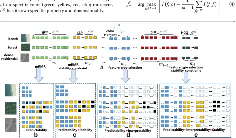
This section presents feature selections and their cor-responding results using different criteria based on predictability, stability, and interpretability, as shown in Fig. 1. Suppose a feature set F with m -dimensional features fl is extracted using l different types for each image, denoted by F = f1,f2,. . .fm
. If the length of a given feature type G(i) is mi dimensions, denotes by G(i) = f(i)
1 ,f
(i)
2 ,. . .,f
(i) mi
,li=1mi = m, then
F can be denoted as FG = G(1),G(2),. . .,G(l) =
f1(1),f2(1),. . .,fm(1l),. . .f
(2)
1 ,f( 2)
2 ,. . .f( 2)
ml ,. . .f
(l)
1 ,f(
l)
2 ,. . .f(
l)
ml
.
As shown in Fig.1a,G(i) represents thei-th feature type with a specific color (green, yellow, red, etc); moreover, G(i)has its own specific property and dimensionality.
For predictability, numerous filter models have been developed in feature selection. For example, Min-Redundancy and Max-Relevance (mRMR) [11], as a pop-ular filter model, adopts the following criterion:
fopt=arg max(D−R) (1)
where fopt denotes the optimal selected feature, D and
R represent feature-class relevance and feature-feature redundancy, respectively. In particular,DandRare com-puted by:
maxD(F,c),D= 1
|F|
fi∈F
I(fi;c) (2)
maxR(F),R= 1
|F|2
fi,fj∈F
Ifi;fj (3)
where|F|represents the dimensionality of the feature set, Ifi;c represents mutual information between individual featurefiin feature setF , and classc,I
fi;fj represents mutual information between two individual featuresfiand
fj in feature setF. From Eqs. (2) and (3), D and R in (1) are computed with the mean value of all feature-class rele-vance and feature-feature redundancy in the feature setF, respectively. In practice, the selection of the feature set can be achieved by near-optimal incremental search methods:
¯
fm=arg max fi∈F−F
⎡
⎣Ifi,c − 1 m−1
fj∈F Ifi,fj
⎤ ⎦ (4)
a
b
c
d
e
Fig. 1Feature selection criteria based on predictability, stability, and interpretability.aldifferent types of feature, corresponding toldifferent colors.
whereFrepresentsm- 1-dimensional feature subset that has been already selected from F. Equation (4) aims to selecting them-th from the candidate feature subsetF−F and implements trade-off between high class relevance and low feature redundancy. As shown in Fig.1b, the fea-tures selected from the same feature type are scattering in terms of ranking, which affects the quantitative evaluation of multiple features, resulting in the lack of interpretabil-ity. In addition, the selected results may greatly change due to data fluctuation.
In addition to predictability, stability is another impor-tant measure in feature selection. Various stability evalu-ation indexes are only used to evaluate feature selection method rather than improve the stability of the method itself [24]. To the best of our knowledge, stability is seldom considered in feature selection criteria. Therefore, stabil-ity constraint is employed in this study to obtain robust selection results:
fopt=arg max(D−R+k×S) (5)
whereSrepresents existing stability evaluation index.kis a parameter, which balances prediction factor(D−R)and stability factorS. Then, the stability evaluation index can be computed by:
S(f,F)= 1 i−1
i−1
j=1
SFf,Fj (6)
SFf,Fj = |
Ff ∩Fj|
|Ff ∪Fj|
(7)
whereFf is the union between the selected features and the optimal featuref to be selected in the current selec-tion,Fj(j=1, 2,. . .,i−1)represents the selected feature subset, and|Ff∩Fj|and|Ff∪Fj|represent the intersection and union between feature setsFf andFj , respectively. Unlike Eq. (1), both predictability and stability are used in the the feature selection criterion of Eq. (5). As shown as in Fig.1c, stability constraint helps obtain consistent results of ranking.
Similar to predictability and stability, interpretability is essential for feature selection [20]. However, mutual infor-mation fails to measure the correlation between different types of features, as multivariate density estimation is hard to accurately estimate. Both Eqs. (1) and (5) fail to select interpretive results. Instead of mutual information, gener-alized correlation coefficient (GCC) is adopted to measure DandRfrom Eqs. (1) to (5) for preserving predictability. Givenv−1 types of featureF¯vG−1= ¯G(1)∩ ¯G(2)∩. . .G¯(v−1) selected from the entire feature set ofltypesFvG−1=G(1)∩ G(2)∩. . .G(v−1), whereG¯(x)denotes thexth selected fea-ture type(x=1, 2. . .,v−1), selecting thevth typeG¯(V) from setFG−FvG−1is based on the following condition:
¯
G(v−1)=arg max
G(j)∈FG−FGv−1 ⎡ ⎢ ⎢ ⎣ρ
G(j),c
− 1
v−1
¯ G(i)∈ ¯FGv−1
ρG(j),G¯(i)
+k×S ⎤ ⎥ ⎥ ⎦
(8)
where ρ represents generalized correlation coefficient between different feature types,G¯(i)thei-th selected fea-ture type, andG(j)denotes a certain feature type from the candidate feature set,FG−FvG−1. Generalized correlation coefficient is degraded to Pearson’s correlation coefficient when the dimensionality ofG¯(i)andG(j)is 1.
In the case of only using GCC in Eq. (8) whenk = 0, the corresponding feature selection takes predictability and interpretability into account, as shown in Fig.1d. The selected features of the same feature type are close to each other while the corresponding ranking may greatly change due to data fluctuation. Ifk = 0 in Eq. (8), it means that the feature selection simultaneously takes predictability, stability, and interpretability into account, which is the so-called SIP-FS method in this paper, as shown in Fig. 1e. From an interpretative point of view, features selected by SIP-FS method are meaningful class-specific features [35] with the use of one-versus-all strategy.
4 SIP-FS algorithm
SIP-FS aims to select a reasonable and compact feature subset for data representation efficiently; thereby, the selected result should be meaningful and insensitive to data fluctuation as well as performing well in prediction accuracy.
SIP-FS is implemented by repeated iteration until sta-ble and selects the feature subset obtained (uses the selected/obtained feature subset) at the last iteration as the final result. For thei-th iteration,k=λ1∗iand the sta-bilitySiis computed by the mean of all stabilities between
FiandFj(j=1, 2,. . .i−1), whereFiandFjrepresent the
i-th and thej-th selected feature subset, respectively.
si= 1 i−1
i−1
j=1
SFi,Fj (9)
where SFf,Fj = ||FFff∪∩FFjj||. The iteration stops until the following condition is satisfied:
DF¯vG+1,c−RF¯vG+1−DF¯vG,c−RF¯vG→0 (11)
The first part could obtain the ranking of feature type; however, in each selected feature type, there may exist redundancy. Therefore, in the second part, the redun-dancy of each feature type is further removed by selecting a subset. Given thatm−1 features are selected from the v-th feature type, the selection of them-th featuref¯m(v)is described as follows.
¯
fm(v)=arg max ⎡ ⎢ ⎣ρG(v)m,c
− 1 v−1
¯ G(i)∈ ¯FGv−1
ρG(v)m,G¯(i)
+k×S
⎤ ⎥ ⎦
(12)
whereG(mv)= ¯G(mv)−1∪fm(v)= ¯f1(v)∪ ¯f2(v)∪...f¯m(v−)1∪fm(v−)1,fm(v) denotes a certain feature in the candidate feature set. For thev-th feature typeG(v), a subset is obtained until other features can not provide additional information, as in the following equation.
DFˆselG ∪ ˆGvm+1,c−RFˆselG ∪ ˆGvm+1
−D
ˆ
FselG ∪ ˆGvm
,c
−R
ˆ
FselG ∪ ˆGvm→0 (13)
whereFˆselG = ˆG(1)∪ ˆG(2)∪...∪ ˆG(v−1),Gˆ(v)
(m+1)= ˆG
(v)
(m)∪¯f
(v) m+1
5 Results and discussions
In this section, extensive experiments are conducted to illustrate the effectiveness of SIP-FS in terms of predictability, stability, and interpretability. Four fea-ture selection methods, mRMR, ReliefF, En-mRMR, and En-Relief, are used for performance comparisons on three publicly available datasets (two web image datasets named MIML [36] and NUS-WIDE-LITE [37], a remote sensing image dataset named USGS21 [38]). mRMR, ReliefF are commonly used filter methods,
Algorithm 1: SIP-FS via feature type selection and stability constraint
Input: Training sampleM, each sample consists ofl types of feature,FG=G(1),G(2), ...,G(l),λ1, λ2
Output:FˆG=Gˆ(1),Gˆ(2), ...,Gˆ(t) 1 i=1;
2 whileEquation 10 is not satisfieddo 3 generating subsample according toλ2; 4 whileEquation 11 is not satisfieddo 5 selectingttypes of feature using Eq. 8; 6 end
7 obtaining thei-th ranking result of feature type
¯
FselG = ¯G(1)∪ ¯G(2)∪. . .∪ ¯G(t);
8 form=1to tdo
9 whileEquation 13 is not satisfieddo
10 selecting feature setGˆ(m)from the m-th
feature typeG¯(m)using Eq. 12;
11 end
12 end
13 obtaining thei-th selected result
ˆ
FG=
ˆ
G(1),Gˆ(2),. . .,Gˆ(t)
;
14 i=i+1; 15 end
while En-mRMR, and En-Relief are two ensemble meth-ods. One versus all strategy is adopted to select class-specific features for SIP-FS as well as other comparison methods.
For the three datasets, different types of feature are used followed by normalization individually. Libsvm [39] is used for training and classification. The images in each dataset are divided into two equal parts, in which one for training and the other for testing. Experiments are randomly repeated 10 times to report the average results.
Fig. 3NUS-WIDE-LITE
Fig. 4USGS21
Table 1Stability comparisons on MIML
Algorithms mRMR ReliefF En-mRMR En-ReliefF SIP-FS
Desert 0.165 0.113 0.179 0.230 0.410
Mountains 0.153 0.139 0.194 0.284 0.399
Sea 0.217 0.144 0.236 0.267 0.353
Sunset 0.224 0.187 0.202 0.245 0.344
Trees 0.161 0.199 0.152 0.184 0.447
Average 0.184 0.156 0.193 0.242 0.391
The top performance in each row is highlightened in boldface
5.1 Datasets
MIML consists of five classes, which are desert, mountain, sea, sunset, and trees. The number of five classes is 340, 268, 341, 261, and 378, respectively. Figure2shows sam-ple images of this dataset. Eight types of feature (a total of 638 dimensions), color histogram, color moments, color coherence, textures, texture coarseness, tamura-texture directionality, edge orientation histogram, and SBN colors are used in experiments. The dimension of these features is 256, 6, 128, 15, 10, 8, 80, and 135, respectively.
NUS-WIDE-LITE contains images from Flickr.com col-lected by the National University of Singapore. In experi-ments, the images with zero label or more than one labels are removed, resulting in a single label dataset which con-tains nine classes: birds, boats, flowers, rocks, sun, tower, toy, tree, and vehicle, as shown in Fig. 3. Five types of feature (a total of 634 dimensions), color histogram, block-wise color moments, color correlogram, edge direction histogram, and wavelet texture are used for experimental evaluation. The dimension of these features is 64, 225, 144, 73, and 128, respectively.
USGS21 contains 21 classes: agricultural, airplane, base-ball diamond, beach, buildings, chaparral, dense resi-dential, forest, freeway, golf course, harbor, intersection, medium density residential, mobile home park, overpass, parking lot, river, runway, sparse residential, storage tanks,
Table 2Stability comparisons on NUS-WIDE-LITE
Algorithms mRMR ReliefF En-mRMR En-ReliefF SIP-FS
Birds 0.119 0.065 0.147 0.132 0.410
Boats 0.113 0.080 0.152 0.133 0.333
Flowers 0.211 0.096 0.213 0.188 0.594
Rocks 0.172 0.090 0.124 0.109 0.491
Sun 0.259 0.165 0.264 0.251 0.501
Tower 0.158 0.066 0.166 0.152 0.449
Toy 0.260 0.113 0.276 0.232 0.457
Trees 0.134 0.061 0.138 0.131 0.302
Vehicle 0.172 0.107 0.150 0.193 0.402
Average 0.178 0.094 0.181 0.169 0.441
The top performance in each row is highlightened in boldface
and tennis courts, as shown in Fig.4. Each class consists of 100 256 × 256-pixels images with the spatial reso-lution of one foot. Five types of feature (a total of 809 dimensions), color moment, HOG, Gabor, LBP, and Gist, extracted by [40] are used for evaluation. The dimension of these features is 81, 37, 120, 59, and 512, respectively.
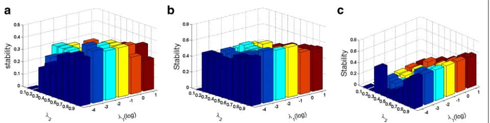
5.2 Effects ofλ1andλ2on stability
In the proposed method, two parameters,λ1andλ2, have influence on the performance of stability.λ1determines the k value, which balances predictability and stability, whileλ2determines the proportion of subsample genera-tion in iterative feature selecgenera-tion. Suitable combinagenera-tion of λ1andλ2is beneficial for obtaining consistent results.
The parameter tuning is conducted for each class indi-vidually. Figure 5 shows the influence of λ1 andλ2 on stability for three different classes, whereλ1is in the range of 0.0001, 0.001, 0.01, 0.1, 1, 10, andλ2 is in the range of 0.1, 0.2, 0.3, 0.4, 0.5, 0.6, 0.7, 0.8, and 0.9, respectively. In general, high stability can be obtained using moderate λ1 value (e.g., 0.001, 0.01, and 0.1 ) and largeλ2(0.8 or 0.9), compared with other parameter combinations. The smallerλ1 value corresponds to better stability, yet the computational complexity is significantly increased. Small
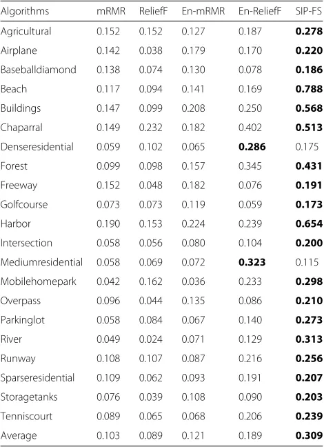
Table 3Stability comparisons on USGS21
Algorithms mRMR ReliefF En-mRMR En-ReliefF SIP-FS
Agricultural 0.152 0.152 0.127 0.187 0.278
Airplane 0.142 0.038 0.179 0.170 0.220
Baseballdiamond 0.138 0.074 0.130 0.078 0.186
Beach 0.117 0.094 0.141 0.169 0.788
Buildings 0.147 0.099 0.208 0.250 0.568
Chaparral 0.149 0.232 0.182 0.402 0.513
Denseresidential 0.059 0.102 0.065 0.286 0.175
Forest 0.099 0.098 0.157 0.345 0.431
Freeway 0.152 0.048 0.182 0.076 0.191
Golfcourse 0.073 0.073 0.119 0.059 0.173
Harbor 0.190 0.153 0.224 0.239 0.654
Intersection 0.058 0.056 0.080 0.104 0.200
Mediumresidential 0.058 0.069 0.072 0.323 0.115 Mobilehomepark 0.042 0.162 0.036 0.233 0.298
Overpass 0.096 0.044 0.135 0.086 0.210
Parkinglot 0.058 0.084 0.067 0.140 0.273
River 0.049 0.024 0.071 0.129 0.313
Runway 0.108 0.107 0.087 0.216 0.256
Sparseresidential 0.109 0.062 0.093 0.191 0.207
Storagetanks 0.076 0.039 0.108 0.090 0.203
Tenniscourt 0.089 0.065 0.068 0.206 0.239
Average 0.103 0.089 0.121 0.189 0.309
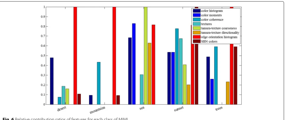
Fig. 6Relative contribution ratios of features for each class of MIML
λ2may result in high fluctuation of subsamples, leading to inconsistent selected results.
5.3 Stability analysis
Tables1, 2, and3show the stability comparisons of five methods on the three datasets. The stabilities of each class and the entire dataset (average) are given in these tables. The stability value ranges from 0 to 1, whereas, “0” and “1” represent the ranking of the selected results are com-pletely inconsistent and consistent in randomly repeated feature selections, respectively.
For Tables 1, 2, and 3, compared with other methods, SIP-FS significantly achieves stability improvement for each class (except for “dense residential” and “medium residential” shown in Table3) as well as the entire dataset, indicating that SIP-FS helps select much more stable features.
In general, mRMR combined with ensemble strategy does not indicate significant improvement in terms of stability. Though ensemble strategy indicates slightly sta-bility advantage for ReliefF, En-ReliefF performs worse than SIP-FS. Overall, SIP-FS performs best on the three datasets in terms of stability.
5.4 Interpretability analysis
Given a certain class, the prediction accuracy varies with feature types. How to select feature types and measure their effectiveness for a specific class are essential for interpretability analysis. In particular, one-versus-all strat-egy are combined with SIP-FS to select feature types (each contains a certain number of features) for a spe-cific class. The effectiveness of these feature types for each class are measured by the relative contribution
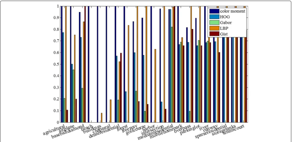
Fig. 8Relative contribution ratios of features for each class of USGS21
ratio, which are normalized by the respective maximum contribution [14].
Figures6,7, and8 show the selected feature types for each class with the respective relative contribution ratio. For example, the selected feature types for “mountain” in MIML are shape and color features, as shown in Fig.6. According to the relative contribution ratios, the selected feature types are edge orientation histogram, color coher-ence, color histogram, and SBN color. The most dis-criminative feature type is shape and the other three are color features (color coherence, color histogram, and SBN colors). However, some texture features (textures, tamura-texture coarseness, and tamura-tamura-texture) and redundant color feature (color moments) are removed. As shown in Fig. 7, color correlogram, edge direction (oriented) histogram, and wavelet texture provide complementary information for describing each class in NUS-WIDE-LITE dataset. In addition, block-wise color moments pro-vide less information for most of classes in this dataset,
Table 4Predictability comparisons on MIML
Algorithms mRMR ReliefF En-mRMR En-ReliefF SIP-FS
Desert 0.735 0.704 0.729 0.727 0.743
Mountains 0.873 0.869 0.834 0.862 0.837 Sea 0.812 0.811 0.786 0.799 0.794
Sunset 0.868 0.829 0.826 0.745 0.859
Trees 0.875 0.839 0.856 0.857 0.854
Average 0.833 0.810 0.806 0.798 0.817
The top performance in each row is highlightened in boldface
while color moments are useless because of the infor-mation redundant. In USGS21 dataset, take the big class road (including freeway, overpass, and runway) and water (including bench and river) as two examples, as shown in Fig.8. LBP is the most discriminative feature type for “road” while color moment is the most discriminative fea-ture type for “water”. Furthermore, as a subclass of water, a river need additional complementary information pro-vided by the other four feature types (LBP, Gabor, HOG and Gist) besides color moment. In general, SIP-FS pro-vides a more interpretive data representation than other comparison methods.
In short, the proposed SIP-FS method provides a more interpretable means for data representation than that of the existing feature selections. More useful information
Table 5Predictability comparisons on NUS-WIDE-LITE
Algorithms mRMR ReliefF En-mRMR En-ReliefF SIP-FS
Birds 0.733 0.686 0.717 0.625 0.725
Boats 0.694 0.653 0.673 0.628 0.702
Flowers 0.834 0.804 0.834 0.808 0.824
Rocks 0.732 0.666 0.735 0.688 0.754
Sun 0.820 0.827 0.807 0.801 0.825
Tower 0.760 0.652 0.749 0.652 0.739
Toy 0.726 0.710 0.733 0.698 0.714
Trees 0.701 0.660 0.688 0.654 0.699
Vehicle 0.761 0.745 0.754 0.687 0.773
Average 0.751 0.711 0.743 0.693 0.751
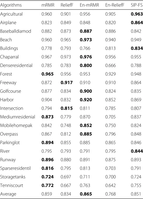
Table 6Predictability comparisons on USGS21
Algorithms mRMR ReliefF En-mRMR En-ReliefF SIP-FS
Agricultural 0.960 0.901 0.956 0.905 0.963
Airplane 0.823 0.849 0.848 0.820 0.864
Baseballdiamod 0.882 0.873 0.887 0.886 0.842
Beach 0.960 0.965 0.973 0.940 0.949
Buildings 0.778 0.793 0.766 0.813 0.834
Chaparral 0.967 0.973 0.976 0.956 0.955 Denseresidential 0.785 0.783 0.800 0.666 0.788
Forest 0.965 0.956 0.953 0.929 0.948
Freeway 0.872 0.917 0.910 0.910 0.864
Golfcourse 0.877 0.834 0.900 0.824 0.835
Harbor 0.904 0.832 0.920 0.852 0.869
Intersection 0.794 0.815 0.811 0.785 0.807 Mediumresidenial 0.873 0.779 0.870 0.705 0.837 Mobilehomepak 0.842 0.748 0.852 0.750 0.824
Overpass 0.867 0.812 0.885 0.796 0.848
Parkinglot 0.894 0.855 0.885 0.865 0.846
River 0.795 0.793 0.791 0.795 0.844
Runway 0.896 0.880 0.891 0.875 0.893
Sparseresidentil 0.816 0.795 0.813 0.703 0.791 Storagetanks 0.724 0.697 0.711 0.700 0.724 Tenniscourt 0.772 0.667 0.763 0.642 0.755
Average 0.859 0.834 0.865 0.768 0.851
The top performance in each row is highlightened in boldface
will become available, deepening the understanding of data.
5.5 Predictability analysis
Tables 4, 5 and6 show the prediction accuracy of each class on the three datasets to evaluate the predictability, respectively. The predictability value ranges from 0 to 1, whereas, “0” and “1” represent completely misclassifica-tion and completely correct classificamisclassifica-tion, respectively.
From Table4, the predictability of mRMR four classes (e.g., mountains, sea, sunset, and trees) of MIML per-forms better than that of other methods. Although SIP-FS performs worse than mRMR in terms of average perfor-mance, it shows advantages than the other three methods. From Table5, mRMR and SIP-FS perform best among all methods in terms of average performance. The compar-ison of mRMR and SIP-FS indicates that both methods have their own accuracy advantages on some classes. For example, the prediction accuracies of SIP-FS on boats, rocks, sun, and vehicle indicate advantages over that of mRMR. From Table6, the average predictability perfor-mances of mRMR, En-mRMR and SIP-FS indicate sig-nificantly advantages over that of the others (ReliefF and En-ReliefF). It is worth noting that although En-ReliefF obtains the highest stability on “dense residential” and “medium residential” (as shown in Table 3), it has the lowest prediction accuracy (as shown in Table6).
In general, SIP-FS and mRMR perform best among all comparison methods on the three datasets, demonstrat-ing that it can maintain good predictability.
To further investigate the effect of the number of selected features on predictability performance, Fig. 9 shows the prediction accuracy of five feature selection methods on three different classes. In general, the predic-tion accuracy of the five methods tends to increase with the number of selected features increases. Desirable pre-diction results can be obtained by selecting the leading features, such as 20 (trees), 30 (flowers), and 20 (building) features, corresponding to Fig.9a–c.
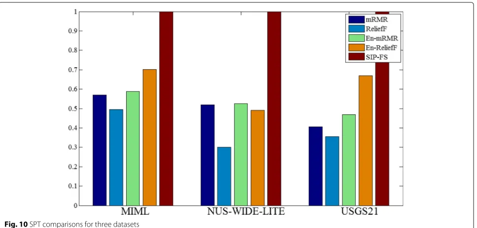
5.6 Trade-off between stability and predictability In the section, stability-predictability tradeoff (SPT) is used to provide a formal and automatic way of jointly eval-uating the trade-off between stability and predictability, as in ref. [29]. The definition of SPT is as follows.
SPT= 2×stability×predictability
stability+predictability (14) where stability (Tables 1, 2 and 3) and predictability (Tables4,5and6) denote the average performance. SPT
Fig. 10SPT comparisons for three datasets
ranges from 0 to 1, the higher the SPT, the better the per-formance. The SPTs for the three datasets are shown in Fig.10. Several conclusions can be drawn from Fig.10: (1) Compared with other methods, SIP-FS can obtain better tradeoff between stability and predictability. (2) mRMR and ReliefF combined with ensemble strategy indicates higher SPT than that without ensemble strategy.
6 Conclusions
In this study, a novel feature selection method called SIP-FS is proposed to explore the stability and interpretability simultaneously while preserving predictability. Given a set of distinct feature types, the relation between different feature types is measured by minimal redundancy max-imal relevance based on generalized correlation. Several feature types can then be selected and used to determine what types contribute to a specific class by quantita-tive evaluation. Furthermore, consistent results of ranking can be achieved through incorporating stability into the criterion of SIP-FS. The experiments on three datasets, MIML, NUS-WIDE-LITE, and USGS21, demonstrate that the performances of stability and interpretability are significantly improved without sacrificing predictability, compared with other filter and their respective ensemble-based methods. In future work, we intend to further investigate the selection of multi-modal information using SIP-FS.
Acknowledgements Not applicable.
Funding
This work was supported by the National Key Basic Research and
Development Program of China under Grant 2012CB719903, the Science Fund for Creative Research Groups of the National Natural Science Foundation of
China under Grant 61221003, the National Natural Science Foundation of China under Grant 41071256, 41571402, and the National Science Foundation of China Youth Program under Grant 41101386.
Availability of data and materials Not applicable.
Authors’ contributions
YG and JJ have implemented the algorithms and performed most of the experiments. HH, TF and DL modified the manuscript. All authors read and approved the final manuscript.
Competing interests
The authors declare that they have no competing interests.
Publisher’s Note
Springer Nature remains neutral with regard to jurisdictional claims in published maps and institutional affiliations.
Author details
1Department of Automation, Shanghai Jiao Tong University, Dongchuan
Road, Shanghai, China.2State Key Laboratory of Information Engineering in
Surveying, Mapping and Remote Sensing, Wuhan University, Luoyu Road, 430079 Wuhan, China.
Received: 28 November 2017 Accepted: 31 January 2018
References
1. T Ojala, M Pietikainen, D Harwood, inProceedings of the 12th International Conference on Pattern Recognition. Performance evaluation of texture measures with classification based on kullback discrimination of distributions (IEEE, New York, 2002), pp. 582–5851
2. TS Lee, Image representation using 2d gabor wavelets. IEEE Trans. Pattern Anal. Mach. Intell.18(10), 959–71 (1996)
3. X Jiang, J Lai, Sparse and dense hybrid representation via dictionary decomposition for face recognition. IEEE Trans. Pattern Anal. Mach. Intell. 37(5), 1067–79 (2015)
4. H Liu, L Yu, Toward integrating feature selection algorithms for classification and clustering. IEEE Trans. Knowl. Data Eng.17(4), 491–502 (2005)
6. PN Belhumeur, JP Hespanha, DJ Kriegman, Eigenfaces vs. fisherfaces: Recognition using class specific linear projection. IEEE Trans. Pattern Anal. Mach. Intell.19(7), 711–720 (2002)
7. F Zamani, M Jamzad, A feature fusion based localized multiple kernel learning system for real world image classification. EURASIP J. Image Video Process.2017(1), 78 (2017)
8. F Poorahangaryan, H Ghassemian, A multiscale modified minimum spanning forest method for spatial-spectral hyperspectral images classification. EURASIP J. Image Video Process.2017(1), 71 (2017) 9. X He, P Niyogi, in17th Annual Conference on Neural Information Processing
Systems (NIPS). Locality preserving projections (MIT PRESS, Cambridge, 2003), pp. 186–197
10. Y Wang, C Han, C Hsieh, K Fan, Vehicle color classification using manifold learning methods from urban surveillance videos. EURASIP J. Image Video Process.2014, 48 (2014)
11. H Peng, F Long, CHQ Ding, Feature selection based on mutual information: criteria of max-dependency, max-relevance, and min-redundancy. IEEE Trans. Pattern Anal. Mach. Intell.27(8), 1226–38 (2005)
12. Y Li, J Si, G Zhou, S Huang, S Chen, FREL: A Stable Feature Selection Algorithm. IEEE Trans. Neural Netw. Learn. Syst.26(7), 1388–1402 (2017) 13. T Le, S Kim, On measuring confidence levels using multiple views of
feature set for useful unlabeled data selection. Neurocomputing.173, 1589–601 (2016)
14. X Chen, T Fang, H Huo, D Li, Measuring the effectiveness of various features for thematic information extraction from very high resolution remote sensing imagery. IEEE Trans. Geosci. Remote Sens.53(9), 4837–51 (2015)
15. Y Sun, Iterative RELIEF for feature weighting: algorithms, theories, and applications. IEEE Trans. Pattern Anal. Mach. Intell.29(6), 1035–51 (2007) 16. CM Bishop,Pattern recognition and machine learning, 5th Edition.
Information science and statistics. (Springer, New Haven, 2007) 17. H Wei, SA Billings, Feature subset selection and ranking for data
dimensionality reduction. IEEE Trans. Pattern Anal. Mach. Intell.29(1), 162–66 (2007)
18. M Dash, H Liu, Consistency-based search in feature selection. Artif. Intell. 151(1-2), 155–176 (2003)
19. I Guyon, A Elisseeff, An introduction to variable and feature selection. J. Mach. Learn. Res.3, 1157–82 (2003)
20. A-C Haury, P Gestraud, J-P Vert, The influence of feature selection methods on accuracy, stability and interpretability of molecular signatures. PLoS ONE.6(12), e28210 (2011)
21. J Li, H Liu, S-K Ng, L Wong, Discovery of significant rules for classifying cancer diagnosis data. Bioinformatics (Oxford, England).19, 93–102 (2003) 22. W Hu, W Li, X Zhang, SJ Maybank, Single and multiple object tracking
using a multi-feature joint sparse representation. IEEE Trans. Pattern Anal. Mach. Intell.37(4), 816–33 (2015)
23. H Wang, F Nie, H Huang, inProceedings of the 30th International Conference on Machine Learning. Multi-view clustering and feature learning via structured sparsity, vol. 28 (JMLR.org, Atlanta, 2013), pp. 1389–1397 24. P Somol, J Novovicová, Evaluating stability and comparing output of
feature selectors that optimize feature subset cardinality. IEEE Trans. Pattern Anal. Mach. Intell.32(11), 1921–39 (2010)
25. PC K. Dunne, F Azuaje, Solutions to instability problems with sequential wrapper-based approaches to feature selection. TCD-CS-2002-28. J. Mach. Learn. Res, 1–22 (2002)
26. A Kalousis, J Prados, M Hilario, Stability of feature selection algorithms: a study on high-dimensional spaces. Knowl. Inf. Syst.12(1), 95–116 (2007) 27. S Loscalzo, L Yu, CHQ Ding, inProceedings of the 15th ACM SIGKDD
International Conference on Knowledge Discovery and Data Mining. Consensus group stable feature selection (ACM, New York, 2009), pp. 567–576
28. M Zucknick, S Richardson, EA Stronach, Comparing the characteristics of gene expression profiles derived by univariate and multivariate classification methods. Stat. Appl. Genet. Mol. Biol.7(1), 95–116 (2008) 29. Y Saeys, T Abeel, YV de Peer, inProceedings of European Conference on Machine Learning and Knowledge Discovery in Databases. Robust feature selection using ensemble feature selection techniques (Springer, Berlin, 2008), pp. 313–25
30. Y Li, S Gao, S Chen, inProceedings of the Twenty-Sixth AAAI Conference on Artificial Intelligence. Ensemble feature weighting based on local learning and diversity (AAAI, Menlo Park, 2012)
31. A Woznica, P Nguyen, A Kalousis, inThe 18th ACM SIGKDD International Conference on Knowledge Discovery and Data Mining. Model mining for robust feature selection (ACM, New York, 2012), pp. 913–921
32. Y Han, L Yu, inICDM 2010, in The 10th IEEE International Conference on Data Mining. A variance reduction framework for stable feature selection (IEEE, Washington, 2010), pp. 206–215
33. L Yu, Y Han, ME Berens, Stable gene selection from microarray data via sample weighting. IEEE/ACM Trans. Comput. Biology Bioinform.9(1), 262–72 (2012)
34. L Yu, CHQ Ding, S Loscalzo, inProceedings of the 14th ACM SIGKDD International Conference on Knowledge Discovery and Data Mining. Stable feature selection via dense feature groups (ACM, New York, 2008), pp. 803–811
35. X Chen, G Zhou, Y Chen, G Shao, Y Gu, Supervised multiview feature selection exploring homogeneity and heterogeneity with l12-norm and automatic view generation. IEEE Trans. Geosci. Remote Sens.55(4), 2074–88 (2017)
36. Z Zhou, M Zhang, inThe Twentieth Annual Conference on Neural Information Processing Systems. Multi-instance multi-label learning with application to scene classification (MIT Press, Cambridge, 2006), pp. 1609–1616
37. T Chua, J Tang, R Hong, H Li, Z Luo, Y Zheng, inProceedings of the 8th ACM International Conference on Image and Video Retrieval. NUS-WIDE: a real-world web image database from national university of singapore (ACM, New York, 2009)
38. Y Yang, SD Newsam, inProceedings of the 18th ACM SIGSPATIAL International Symposium on Advances in Geographic Information Systems. Bag-of-visual-words and spatial extensions for land-use classification (ACM, New York, 2010), pp. 270–279
39. C Chang, C Lin, LIBSVM: A library for support vector machines. ACM TIST. 2(3), 27–12727 (2011)