Modelling the concentration dependence of doping in optical materials.

This content has been downloaded from IOPscience. Please scroll down to see the full text.

Download details:

IP Address: 160.5.62.96

This content was downloaded on 17/12/2015 at 09:17

Please note that terms and conditions apply.

Modelling the concentration dependence of doping in optical materials

View the table of contents for this issue, or go to the journal homepage for more 2015 IOP Conf. Ser.: Mater. Sci. Eng. 80 012010

(http://iopscience.iop.org/1757-899X/80/1/012010)

Modelling the concentration dependence of doping in optical

materials

R A Jackson1_{, M E G Valerio}2

1. School of Physical and Geographical Sciences, Keele University, Keele, Staffordshire ST5 5BG, UK

2. Department of Physics, Federal University of Sergipe, 49.100-000 São Cristóvão, Brazil

E-mail: [email protected]

Abstract. As well as understanding the location of dopants in optical materials, it is also important to understand how much dopant can be added to a given material. A method for calculating the maximum concentration of dopants has been developed, and applied to dopants in mixed metal fluorides for optical and nuclear clock applications. Applications to rare earth doping in YLiF4, and Th doping in LiCaAlF6/LiSrAlF6 are described, and compared with

available experimental data.

1.Introduction

This paper is part of an ongoing modelling study of dopants in optical materials. Previous papers have addressed the question of where dopants are located in the host lattice (see e.g. [1]) and their effect on morphology [2], and an initial study of concentration dependence of dopants has been published [3].

The motivation for this study is to develop a method by which the maximum concentration of a given dopant in a host lattice can be predicted. This is useful information for device development and can potentially save time in crystal growth experiments.

The paper starts with a description of the method to be used, using rare earth doping in YLiF4 as an example, and it is then applied to the doping of LiCaAlF6/LiSrAlF6 and CaF2 with 229_{Th ions, which is} relevant to the development of nuclear clocks using these materials discussed previously [4, 5].

2. Methodology and Results

2.1 The doping process for rare earth ions in YLiF4

1

To whom any correspondence should be addressed.

Doping YLiF4 with rare earth (M3+) ions can be represented as follows (where doping at the Y site is assumed), and x is the mole fraction of dopant:

(1-x) YF3 + x MF3 + LiF → Y1-xMxLiF4

The energy of this reaction corresponds to the solution energy of the doping process, Esol:

Esol = E (Y1-xMxLiF4) - [(1-x) Elatt (YF3) + x Elatt (MF3) + Elatt (LiF)]

The terms in square brackets are calculated lattice energies, Elatt, and the only issue is in calculating the first term in the equation. This has been done using the equation below, which effectively splits the defective lattice energy into a perfect lattice component Ep (1) and a defect formation energy term EDML :

ED(x) = x EDML + Ep (1)

The final solution energy expression then becomes:

Esol = E (x EDML _{+ Elatt (YLiF4)) - [(1-x) Elatt (YF3) + x Elatt (MF3) + Elatt (LiF)]}

Here the term EDML is the substitution energy of an M3+ cation at the Y3+ site.

Using this expression, maximum dopant concentrations in mol % have been calculated for rare earth ions in YLiF4, as given in table 1. These correspond to the value of ‘x’ when Esol = 0.

Table 1. Calculated maximum dopant concentrations for rare earth ions in YLIF4 [6]

Ion Max. mol % Ion Max. mol %

La 0.69 Tb 1.41

Ce 0.76 Dy 1.28

Pr 0.85 Ho 1.40

Nd 0.93 Er 1.52

Sm 1.23 Tm 1.33

Eu 1.15 Yb 1.51

Gd 1.22 Lu 1.49

2.2 Th4+ _{doping in LiCaAlF} 6

In a previous paper [4] the doping of LiCaAlF6 with Th4+ has been discussed in the context of developing a ‘nuclear clock’ material which exploits the unusually low first nuclear excited state energy of the 229_{Th isotope. It is necessary to embed the Th in a transparent crystal, and the} calculations predict that Th4+ _{will substitute at the Ca}2+ _{site with charge compensation by the} formation of two F- _{interstitials. The doping process is therefore assumed to follow this reaction:}

x ThF4 + (1-x) CaF2 + LiF + AlF3 → LiThxCa1-xAlF6+2x

Using the approach described in 2.1, this leads to a solution energy expression as follows:

Esol = E (LiThxCa1-xAlF6+2x) – [x Elatt (ThF4) + (1-x) Elatt (CaF2) + Elatt (LiF) + Elatt (AlF3)]

12th Europhysical Conference on Defects in Insulating Materials (EURODIM 2014) IOP Publishing IOP Conf. Series: Materials Science and Engineering80(2015) 012010 doi:10.1088/1757-899X/80/1/012010

Which leads to:

Esol = E (x ED ML

+ Elatt (LiCaAlF6)) - [x Elatt (ThF4) + (1-x) Elatt (CaF2) + Elatt (LiF) + Elatt (AlF3)]

Now the term ED ML

is the energy of substitution of the Th4+ ion at the Ca2+ site, plus the energy of formation of two F- interstitials.

Setting Esol = 0 a value of x =0. 06 or 6 mol% is obtained for the maximum dopant concentration of Th4+ ions in LiCaAlF6. Experiments are in progress to test these conclusions.

2.3 Th4+ doping in CaF2

Th4+ doping in CaF2 was considered in [5], where it was again found that the predicted location of the dopant Th4+ would be at the Ca2+ site, with charge compensation by F- interstitials. The doping scheme is assumed to be:

x ThF4 + (1-x) CaF2  Ca1-xThxF2+2x

The corresponding expression for the solution energy is:

Esol = E (Ca1-xThxF2+2x) – [x Elatt (ThF4) + (1-x) Elatt (CaF2)]

This can be written as:

Esol = E (x ED ML

+ Elatt (CaF2)) - [x Elatt (ThF4) + (1-x) Elatt (CaF2)]

For binary systems like CaF2 a minimum value of ‘x’ is not calculated, but it is possible to calculate Esol as a function of x. Preliminary experimental measurements [7] suggest dopant concentrations of between 0.4-0.7 mol%, corresponding to solution energies in the range 2.3 – 3.5 eV. These values are of the same order of magnitude as solution energies calculated for many doping processes in optical materials. However, more detailed measurements are in progress, and a detailed comparison will be reported in a later publication.

3. Conclusions

This paper has presented a method for predicting the maximum concentration of dopants in optical materials, and has been applied to two representative systems. It is expected that the method will be further refined once more experimental data is available, but in its present form reliable predictions have been made.

4. References

[1] Maddock E M, Jackson R A and Valerio M E G 2010 J. Phys.: Conference Series249 012040

[2] Littleford T E, Jackson R A and Read M S D 2013 Phys. Stat. Sol. C10 (2) 156

[3] Rezende M V S, Valerio M E G and Jackson R A 2011 Optical Materials34 109

[4] Jackson R A, Amaral J B, Valerio M E G, DeMille DP and Hudson E R 2009 J. Phys.: Cond.

Matt. 21 325403

[5] Dessovic P, Mohn P, Jackson R A, Winkler G, Schreitl M, Kazakov G and Schumm T 2014J.

Phys.: Cond. Matt. 26 105402

[6] LittlefordT E 2014 PhD thesis, University of Keele, UK

[7] Schumm T private communication

Acknowledgements

MEGV is grateful to CNPq (Conselho Nacional de Desenvolvimento Científico e Tecnológico) for research support.

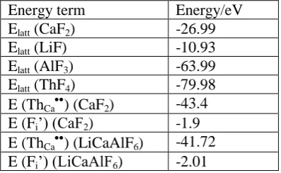
Appendix

Table of lattice energies and defect formation energies used in sections 2.2 and 2.3

Energy term Energy/eV

Elatt (CaF2) -26.99

Elatt (LiF) -10.93

Elatt (AlF3) -63.99 Elatt (ThF4) -79.98 E (ThCa) (CaF2) -43.4 E (Fi’) (CaF2) -1.9 E (ThCa) (LiCaAlF6) -41.72 E (Fi’) (LiCaAlF6) -2.01

12th Europhysical Conference on Defects in Insulating Materials (EURODIM 2014) IOP Publishing IOP Conf. Series: Materials Science and Engineering80(2015) 012010 doi:10.1088/1757-899X/80/1/012010