R E V I E W
Open Access
Generating discrete analogues of
continuous probability distributions-A
survey of methods and constructions
Subrata Chakraborty
Correspondence: [email protected] Department of Statistics, Dibrugarh University, Dibrugrah 786004, Assam, India
Abstract
In this paper a comprehensive survey of the different methods of generating discrete probability distributions as analogues of continuous probability distributions is presented along with their applications in construction of new discrete distributions. The methods are classified based on different criterion of discretization.
Keywords:Discrete analogue; Reliability function; Hazard rate function; Competing risk; Exponentiated distribution; Maximum entropy; Discrete pearson; T-X method
1. Introduction
Sometimes in real life it is difficult or inconvenient to get samples from a continuous distribution. Almost always the observed values are actually discrete because they are measured to only a finite number of decimal places and cannot really constitute all points in a continuum. Even if the measurements are taken on a continuous scale the observations may be recorded in a way making discrete model more appropriate.
In some other situation because of precision of measuring instrument or to save space, the continuous variables are measured by the frequencies of non-overlapping class inter-val, whose union constitutes the whole range of random variable, and multinomial law is used to model the situation.
In categorical data analysis with econometric approach existence of a continuous un-observed or latent variable underlying an un-observed categorical variable is presumed. Categorical variable is the observed as different discrete values when the unobserved continuous variable crosses a threshold value. Therefore, the inference is based on ob-served discrete values which are only indicative of the intervals to which unobob-served continuous variable belongs but not its true values. Hence this is a case where one makes use of a discretization of the underlying continuous variable.
In survival analysis the survival function may be a function of count random variable that is a discrete version of underlying continuous random variable. For example the length of stay in an observation ward is counted by number of days or survival time of leukemia patients counted by number of weeks. From these examples it is clear that the continuous life time may not necessarily always be measured on a continuous scale but may often be counted as discrete random variables.
More over often the continuous failure time data generated from a complex sys-tem poses more derivational problem than that of a discrete version of the under-lying continuous one. Despite these discrete life time distributions played only a marginal role in reliability analysis. Therefore, there is a need to focus on more realistic discrete life time distributions (Rezaei Roknabadi et al. 2009). That is discretization of a continuous lifetime model is an interesting and intuitively ap-pealing approach to derive a discrete lifetime model corresponding to the continu-ous one (Lai 2013).
From the above discussion it can be inferred that many a times in real world the ori-ginal variables may be continuous in nature but discrete by observation and hence it is reasonable and convenient to model the situation by an appropriate discrete distribu-tion generated from the underlying continuous models preserving one or more import-ant traits of the continuous distribution.
Deriving discrete analogues (Discretization) of continuous distribution has drawn at-tention of researchers. In recent decades a large number of research papers dealing with discrete distribution derived by discretizing a continuous one have appeared in a scattered manner in existing statistical literatures.
There are several ways to derive discrete distribution from continuous ones. In the current published literature we could find only two papers that dealt with surveys of discrete analogues of continuous distributions though in a limited manner. These are Bracquemond and Gaudoin (2003) who devoted a section on discrete life time dis-tributions derived from continuous one in their survey on discrete life time distri-butions and Lai (2013) who presented construction of discrete lifetime distributions from continuous one in his paper concerning issues of construction of discrete life time distribution
With above background the main motivation of this article is to present a com-prehensive method-wise survey of the different techniques of discretization of con-tinuous distributions, with examples of their applications in construction of discrete analogues.
In the section 2 of this article discretization of continuous distributions are discussed method wise including composite methods, which comprise two stages using two dif-ferent methods in separate subsections. In section 3 a discussion on the discretization highlighting its need, limitations and also a final conclusion is presented. Throughout the paper continuous random variable to be discretized is denoted by X while its discrete analogue by Y and with respect to discrete life time characteristics Kemp’s (2004) convention is followed.
2. Discrete analogues
A continuous random variable may be characterized either by its probability density func-tion (pdf), moment generating funcfunc-tion (mgf ), moments, hazard rate funcfunc-tion etc. Basic-ally cconstruction of a discrete analogue from a continuous distribution is based on the principle of preserving one or more characteristic property of the continuous one.
The various methods by which discrete analogue Yof a continuous random variable
I. Difference equation analogues of Pearsonian differential equation.
II. Probability mass function (pmf ) ofYretains the form of the pdf ofXand support ofYis determined from full range ofX.
III. Pmf ofYretains the form of the pdf ofXand support ofYis determined from a subset of the range ofX.
IV. Survival function (sf ) ofYretains the form of the survival function ofXand support ofYis determined from full range ofX.
V. Cumulative distribution function (cdf ) ofYretains the form of the cdf ofXand support ofYis determined from a subset of the range ofX.
VI. Hazard (failure) rate function ofYretains the form of the hazard (failure) rate function ofX.
VII. Moments ofYandXup to a certain order coincides.
VIII. Any interval domain, any theoretically possible mean–variance pair forY IX. Two stage composite methods
2.1 Discrete analogue of pearsonian system
Pearson (1895) starting with the difference equation
pk−pk−1 pk ¼
k−a b0þb1kþb2k2
ð1Þ
defined the celebrated Pearsonian system of continuous distributions with pdf satisfy-ing the differential equation
1
f df dx¼
aþx c0þc1xþc2x2
Though Pearson himself did not pursue the development of a discrete analogue of his continuous system, the difference Eq. in (1) was used by Carver (1919, 1923). But he too did not attempt a thorough examination of the discrete distributions arising from Eq. (1).
Katz (1945, 1946, 1948, 1965) developed a discrete analogue of the Pearsonian system of continuous distributions by using the relationship
pkþ1¼
aþbk
1þk pk; k¼0; 1; 2; …
Where pk=P(Y=k). The main motivation of Katz was to discriminate between
bino-mial, Poisson and negative binomial distributions. Some notable related developments following Katz are as follows:
Ord (1967a,b,c,1968) discussed discrete analogue of the Pearson continuous system by using the following difference equation:
pk−pk−1
pk ¼
a−k aþb0
ð Þ þðb1−1Þkþb2k k−ð 1Þ
pk¼αm=Y
m
j¼1
jþkþa
ð Þ2þ
b2
;k∈Z
Where 0≤a≤1, 0 <b<∞, m is a non negative integer, and αm is a normalizing
con-stant. (see Johnsonet al.2005for detail).
Gurland and Tripathi (1975) and Tripathi and Gurland (1977), studied the extended Katz family that satisfies the probability recurrence relation
pkþ1¼
aþbk
cþk pk; k¼0; 1; 2; …
Sundt and Jewell (1981) investigated a family of distributions satisfying probability recurrence relation
pkþ1¼
aþbþak
1þk pk; k¼0; 1; 2; … (See also Willmot,1988)
2.2 Methodology-II
In this method the pmf of the discrete random variable Yis derived as an analogue of the continuous random variableXwith pdff(x),− ∞<x<∞as
P Yð ¼kÞ ¼f kð Þ=X
∞
j¼−∞
f jð Þ; k¼0;1;2;⋯ ð2Þ
The distribution generated using this technique may not always have a compact form due to the normalizing constant.
2.2.1 Good distribution
The first trace of this type of construction is seen in Good distribution (Good 1953) having pmf
P Yð ¼kÞ ¼qkka=X
∞
j¼1
qjja; k¼1; 2;⋯; α∈R ð3Þ
When a>−1, this distribution can be derived as a discrete analogue of gamma distri-bution by considering
f xð Þ ¼θβ1Γβxβ−1e−x=θin Eq. (2) and replacinge−1/θ=qandβ−1 =a.
This distribution was applied to model the population frequencies of species and the estimation of population parameters.
This distribution was extensively studied by Kulasekara and Tonkyn (1992) and Doray and Luong (1997).
The distribution in Eq. (3) is a special case of Hurwtiz-Lerch Zeta Distribution (Zornig and Altmann 1995; Doray and Luong 1997; Gupta et al. 2008). For Hurwtiz-Lerch Zeta functions see Gradshteyn and Ryzhik (2000). (see also section 11.2.20 of Johnson et al. 2005).
Another related distribution is the discrete Pareto distribution, also known as the Riemann zeta distribution (see page 527, Johnsonet al. 2005).
2.2.2 General Dirichlet distribution
Using general Dirichlet series, Siromoney (1964) studied the general Dirichlet Series distribution with pmf
P Yð ¼kÞ ¼ake−λkθ
X∞
j¼1
aje−λjθ; k¼1; 2;⋯;
Various distributions were seen as particular cases as follows:
Forλk= log(k), the distribution reduces toDirichlet series distributionwith pmf
P Yð ¼kÞ ¼akk−θ
X∞
j¼1
ajj−θ; k¼1; 2;⋯
Forak=aandλk= log(k), the distribution reduces toZeta distributionwith pmf
P Yð ¼kÞ ¼k−θ=ζ θð Þ; k¼1; 2; … where ζ θð Þ ¼X
∞
j¼1
j−θ is the Riemann Zeta
function.
Puttingλk=k, e−θ=α, givespower seriesdistribution with pmf
P Yð ¼kÞ ¼akαkX
∞
j¼0
ajαj; k¼0;1; 2;⋯
Forak=ka, e−θ=qandλk=−kreduces toGood distribution
Forak=k, λk=−k2andθ= 1/2discrete Pearsondistribution mentioned in Byers and Shenton (1994) having pmf
P Yð ¼kÞ∝ke−k2=2;k¼1; 2;⋯
Thediscrete Pearson IIIdistribution of Haight (1957) is a special
case withak= (k+ν)aandλk=k(page 532, Johnsonet al.2005) with pmf
P Yð ¼kÞ ¼e−kθ=½ðkþνÞaX
∞
j¼0
e−jθ=ðjþνÞa
; k¼0;1; 2;⋯
Siromoney (1964) applied this distribution to model frequency distribution of the length of wet spells during the period 1932-62 in a place called Tambaram in southern India.
2.2.3 Discrete normal distribution
The discrete normal distribution was derived as a discrete analogue of the normal
distribution (Kemp 1997) by considering f xð Þ ¼σp1ffiffiffiffi2πexp −ðx−μÞ2 2σ2
h i
; in Eq. (2) and
sub-stituting,eð1−2μÞ=2σ2
¼λande−1=σ2
¼q:The resulting pmf is given by
P Yð ¼kÞ ¼λkqk k−ð 1Þ=2X
∞
j¼−∞
λjqj j−ð 1Þ=2; k¼0;1;2;⋯ ð4Þ
This distribution is characterized by maximum entropy for specified mean and vari-ance, and integer support on (−∞, +∞). It can be derived as the distribution of the dif-ference of two related Heine distribution (Benkherouf and Bather 1988; see also section 4.12.6 of Johnsonet al.2005 and references therein)
Weighted distribution of discrete normal with parameter (λ,q) with weight function of the formπxis again discrete normal (πλ,q).
Forλ=q1/2andq=e−2βthe pmf in Eq. (4) reduces to that of Das Gupta (1993) ver-sion ofdiscrete normaldistribution.
P Yð ¼kÞ ¼qk=2e−βk k−ð 1ÞX
∞
j¼−∞
qj=2e−βj j−ð 1Þ; k¼0;1;2;⋯
The distribution is log concave and unimodal like normal distribution.
Harris et al. (2001)applied this distribution in dynamic analysis of rural retail estab-lishment count data.
2.2.4 Discrete exponential distribution
Sato et al. (1999) proposed discrete exponential distribution having similar looking structure starting with the continuous exponential distribution having pdf
f xð Þ ¼λe−λx; x>0;α>0;λ>0:
The pmf of their discrete exponential distribution was
P Yð ¼kÞ ¼1−e−λe−λk; k¼0; 1; 2;⋯: ð5Þ
This is the geometric distribution with pmf
P(Y=k) = (1−p)pk,k= 0, 1, 2,⋯, wherep=e−λ.
Sato et al. (1999)applied this distribution to model defect count distribution in semi-conductor deposition equipment and defect count distribution per chips.
It can be easily checked that the pmf in Eq. (5) can be derived as a discrete analogue of exponential distribution by considering f(x) =λe−λx,x> 0, in Eq. (2).
2.2.5 Discrete Gamma distribution
Sato et al. (1999) also briefly discussed the convolution of their discrete exponential distribution to present a discrete Gamma distribution having pmf
P Yð ¼kÞ ¼
Y m−1
i¼1
kþi
ð Þ
m−1
ð Þ! 1−e−λ
m
e−λk;k¼0; 1; 2;⋯:
P Yð ¼kÞ ¼ mþk−1 k
pkð1−pÞm; k¼0; 1; 2;⋯ when p¼e−λ:
Sato et al. (1999)applied this distribution to model defect count distribution in semi-conductor deposition equipment and defect count distribution per chips.
2.2.6 Discrete log normal distribution
Considering f xð Þ ¼ 1
xσpffiffiffiffi2π exp −
lnx−μ ð Þ2
2σ2
h i
in Eq. (2), Bi et al.(2001) proposed a discrete
distribution with pmf
P Yð ¼kÞ ¼e−ðlnk2σ−2μÞ=kX
∞
j¼1
e−ðlnj2σ−2μÞ; k¼1; 2;⋯ ð6Þ
and called it discrete Gaussian exponential (DGX) distribution. It is easy to see that Eq. (6) can be derived as a discrete analogue of log normal distribution.
This distribution reduces to a discrete generalised Zipf distribution in limit asμ→− ∞ (see Biet al.2001) with pmf
P Yð ¼kÞ∝1 kexp −
lnk−μ
ð Þ
σ2
∝k−ð1−μ=σ2Þ
This distribution was applied to model four extremely skewed count data sets namely Text data from the English Bible, Sales data from a large retailer chain, Telecommuni-cations data customer data from an AT&T service of monthly usage volumes, and Click stream data and browsing behavior of internet users.
2.2.7 Discrete half normal distribution
Kemp (2006) presented a discrete half normal distribution as a maximum entropy dis-tribution for given mean and variance with support 0, 1, 2⋯. The pmf is given by
P Yð ¼kÞ ¼θkqk k−ð 1Þ=2X
∞
j¼0
θjqj j−ð 1Þ=2; k¼0; 1; 2;⋯:
This can be seen as discretization of continuous half normal in the same way as in section 2.2.3. It can arises as a limiting q-hyper-Poisson-I (Kemp 2002) distribution and also as a mixture ofHeinedistributions (Benkherouf and Bather 1988).
Khorashiadizadeh et al. (2012) referred this distribution asdiscrete truncated normal. For an approximation result on this distribution see Byers and Shenton (1994).
2.2.8 Discrete Laplace (double exponential)
Inusah and Kozubowski (2006) proposed a discrete analogue of Laplace (Double expo-nential) distribution having pmf
P Yð ¼kÞ ¼ 1−p
1þpp
k
j j; k¼0;1;2;⋯; 0<p<1; ð7Þ
This distribution can be derived as a discrete analogue of Laplace distribution by considering
f xð Þ ¼ 1
2σ expð−j jx=σÞ;in Eq. (2) and substituting,e−1/σ=p.
Inusah and Kozubowski (2006) applied this distribution in modelling different currency exchange rate data. Meyer et al. (2013) applied it for estimating Y-STR haplotype frequencies.
2.2.9 Discrete Skew Laplace
Considering skew Laplace distribution with pdf
f xð Þ ¼1
σ
m
1þm2
expð−xm=σÞ;x≥0 expð−x=mσÞ;x<0
as the base distribution, a discrete analogue was first proposed by Kozubowski and Inusah (2006). It’s pmf is given by
P Yð ¼kÞ ¼ð1−pÞð1−qÞ
1−p q
pk ; k¼0; 1;2; 3; …
qj jk ; k¼0;−1;−2;−3; …
ð8Þ
Wheree−1/σ=pande−1/kσ=q,pє(0, 1) andqє(0, 1).
Forp=qEq. (8) reduces to Eq. (7). Arises as the difference of two independently but not identically distributed geometric random variables.
This distribution was also applied for modeling currency exchange rates.
Another discrete distribution that generalizes the discrete skew Laplace distribution was proposed by Lekshmi and Sebastian (2014). This newGeneralized Discrete Laplace dis-tribution can be derived as the difference of two independently distributed negative
binomial(NB) random variables with same dispersion parameter.
2.2.10 Discrete generalized exponential distribution
The generalized exponential distribution of Gupta and Kundu (1999) has pdf
f xð Þ ¼αλ1−e−λxα−1e−λx; x>0;α>0;λ>0:
A discrete analogue of this distribution was proposed by Nekoukhou et al. (2012) with pmf
P Yð ¼kÞ ¼C pk−11−pkα−1=X ∞
j¼0 α−1
j
−1
ð Þj
1−p1þj; k¼1;2;3;⋯
WhereC¼X ∞
j¼0 α−1
j
−1
ð Þj pj
1−p1þj; e−λ¼p
Nekoukhou et al. (2012)applied this distribution to model rank frequencies of graph-emes in a Slavic language called‘Slovene’.
Among the various distribution described in section 2.2 above, discrete normal in section 2.2.3, discrete half normal in section 2.2.7 and discrete Laplace distribution in section 2.2.8 can also be classified as generated to preserve the maximum entropy
2.3 Methodology-III
This is a modification of the method-II (Barbiero 2010). Here the discrete analogue is derived to have a finite support.
Suppose X is a continuous random variable with pdf fX(x),− ∞<x<∞. Y is the discrete analogue with the support consisting of kpoints to be derived from the range ofX. Letg= (1−k)/2,kodd positive integer andyi=g−1 +i,i= 1, 2,⋯,k.
For an example consider the case of discretizing X. Let ci¼Φð Þyi ; yi¼F−X1ð Þci ;
whereΦ(yi) is the cdf ofN(0, 1) andFX() is the cdf of theX. Then the pmf ofYwith support {y1,y2,⋯,yk} is given by
P Yð ¼yiÞ ¼fXð Þyi X
k
i¼1
fXð Þ;yi i¼1; 2;⋯;k
Barbiero (2010) gave examples of discrete gamma with 5 points and Weibull with 9 points support.
This method generates discrete analogue of continuous distribution with limited sup-port like beta distribution. Here if Xis symmetrical thenYretains expected value ofX
and pmf ofYretains the structure of the pdf ofX.
For this method to be implemented the continuous cdf must be invertible, the sup-port of the resulting discrete distribution may not be set of integers.
Barbiero (2010) has applied this method to estimate the reliability of systems for which stress and strength are defined as complex functions, and whose reliability is not derivable through analytic techniques.
2.3.1 Discrete power function distribution
The pdf of the continuous finite range power-function distribution having pdf
f xð Þ ¼p xp−1=θp; 0<x<θ;p>0;θ>0
was introduced by Mukherjee and Islam (1983). Lai and Wang (1995) discretized the above distribution to derive a finite range discrete distribution with pmf
P Yð ¼kÞ ¼kα=c Nð ;αÞ;k¼0;1;⋯;N;α>0; α∈R
Where c nð ;jÞ ¼X n
k¼0
kα¼Bjþ1ðnþ1Þ−Bjþ1
jþ1 ; Bmð Þx is the i
th
Bernoulli Polynomial defined
asBmð Þ ¼x X m
k¼0
Bkð Þx xm−k:
This distribution can model bathtub-shaped hazard rate as well as upside-down bathtub-shaped mean residual life. They studied various other reliability properties and applied this model to fit a mortality data.
2.4 Methodology-IV
Following Kemp’s (2004) convention here we consider the definition of the discrete sf defined asSY(k) =P(Y≥k) and accordingly the cdfFY(k) =P(Y≤k) is related to the sf as
SY(k) = 1−FY(k−1).
P Yð ¼kÞ ¼P k≤Xð <kþ1Þ
¼FXðkþ1Þ−FXð Þ ¼k SXð Þ−k SXðkþ1Þ; k¼0;1; 2;… ð9Þ
[Since for continuous random variableX,P(X=x) = 0 andFX(k) = 1−SX(k)]
The method can be viewed deriving a discrete concentration (Roy 2003) of the ran-dom variableXand also as a process of time discretization (Bracquemond and Gaudoin 2003) in the context of X representing life. It is possibly the easiest method of construction.
The resulting pmf will be in a compact form if the continuous sf is in compact form. This method preserves the sf that isSY(k) =SX(k).
One limitation of this technique is the concentration on the left limit of the equal in-tervals in which the support of the continuous random variable is partitioned.
Alternatively, by considering Y=⌈X⌉smallest integer greater than or equal toX one can get a discrete version ofXwith following pmf that will preserve the cdf.
P Yð ¼kÞ ¼P Xð ¼kÞ ¼P kð −1<X≤kÞ
¼P Xð ≤kÞ−P Xð ≤k−1Þ ¼FXð Þ−k FXðk−1Þ; k¼0;1; 2;…
(see Lai 2012; Bracquemond and Gaudoin 2003). It may be noted here that =⌈X⌉=⌊X⌋+ 1.
2.4.1 Discrete exponential distribution
If the underlying distribution is exponential with sf
SXð Þ ¼x P X≥xð Þ ¼ expð−θxÞ;
then the pmf of its discrete version is given by
P Yð ¼kÞ ¼ expð−θkÞ−expð−θðkþ1ÞÞ ¼qk−qkþ1¼ð1−qÞqk;k¼0;1;2;…
where q= exp(−θ). This is the geometric distribution (Bracquemond and Gaudoin
2003).
2.4.2 Discrete Weibull distribution
Weibull distribution is widely accepted failure model but in practice, the failure data are often measured in discrete time such as cycles, blows, shocks, or revolutions. Discrete Weibull was proposed to find a discrete distribution corresponding to the Weibull.
IfX~ Weibull distribution with pdf and sf
fXð Þ ¼x β
λ
x
λ β−1
expn−ðx=λÞβo and SXð Þ ¼x exp −ðx=λÞβ
n o
Considering the sf of the Weibull in the Eq. (9), and substitutingq= exp[(−1/λ)β], Naka-gawa and Osaki (1975) first proposed discrete Weibull distribution with pmf
P Yð ¼kÞ ¼qkβ−qðkþ1Þβ;k¼0;1;2;⋯;β>0; 0<q<1 ð10Þ
Khan et al.(1989) and Kulasekara (1994) considered estimation of this distribution. Englehardht and Li (2011) applied this distribution in modeling microbial counts. See also Bakouchet al.(2012) and Khorashiadizadeh et al. (2012) for applications.
2.4.3 Discrete geometric Weibull distribution
Often we see systems possessing two phase life. First the stable phase having a constant failure rate until the change point timeτfollowed by next step which is the wear out phase with a larger increasing failure rate. Zacks (1984) considered the failure distribution in the wear out phase as Weibull to obtain the sf of the exponential Weibull distribution as
SXð Þ ¼x exp −λx− λðx−τÞþ
β
h i
; where Xþ¼ max 0ð ;XÞ:
The corresponding discrete version referred to as the discrete geometric Weibull was proposed by Bracquemond and Gaudoin (2003) with pmf
P Yð ¼kÞ ¼ exp −λðk−1Þ−λðk−τ−1Þþβ−exp −λk−λðk−τÞþβ h
h
2.4.4 Discrete normal distribution
Roy (2003) considered discrete normal distribution with pmf
P Yð ¼kÞ ¼Φððkþ1−μÞ=σÞ−Φððk−μÞ=σÞ; k¼0;1;2;⋯;σ>0;−∞<μ<þ∞
whereΦ(.) is the cumulative distribution function (cdf ) of standard normal distribution. An application of the distributions for evaluating the reliability of complex systems was elaborated as an alternative to simulation methodsRoy (2003).
2.4.5 Discrete Rayleigh distribution
IfX~ Rayleigh distribution then its pdf and sf are respectively given by
fX(x) = (x/σ2) exp[−x2/2σ2] and sfSX(x) = exp[−x2/2σ2], x> 0. Discrete Rayleigh distribution (Roy 2004) has pmf
P Yð ¼kÞ ¼θk2−θðkþ1Þ2;k¼0;1;2;⋯; 0<θ<1:
This is a particular case of the discrete Weibull distribution of Nakagawa and Osaki (1975) stated in section 2.4.2.
Roy (2004) applied this distribution in reliability modeling and in approximating probability integrals arising out of a reliability analysis in continuous setting.
2.4.6 Discrete Maxwell distribution
IfX~ Maxwell distribution then its pdf and sf are respectively given by
fXð Þ ¼x 4ffiffiffi
π p 1
θ3=2x2e−x 2=θ
and sfSXð Þ ¼x 1−Γð3Γ=ð23;=x22Þ=θÞ; x>0:
Krishna and Pundir (2007) studied discrete Maxwell distribution having pmf
P Yð ¼kÞ ¼ 4ffiffiffi
π
p 1
θ3=2Q kð ;2;θÞ;k¼0; 1; 2;⋯; θ>0
whereQ kð ;2;θÞ ¼ ∫
kþ1
k u 2e−ðu2=θÞ
2.4.7 Discrete extended exponential distribution (Telescopic)
IfX~ extended exponential distribution then its pdf and sf are respectively given by
fXð Þ ¼x αg=θð Þx e−αg=θð Þx;and sfSXð Þ ¼x e−αgθð Þx; α;x>0:
Where gθ(x) is a strictly increasing function of x with gθ(0) = 0 and gθ(x)→∞ as x→∞(Rezaei Roknabadi 2000, 2006).
Rezaei Roknabadi et al. (2009) obtained the pmf of their telescopic distribution by discretizing the extended exponential distribution as
P Yð ¼kÞ ¼qgθð Þk−qgθðkþ1Þ;k¼0;1;2;⋯;whereq=e−α, 0 <q< 1
Rezaei Roknabadiet al. (2009) have shown that this family of distribution belongs to IFR (increasing Failure Rate) class if any one of the following is true:
i. gθð Þ ¼y gθðyþ1Þ−gθð Þy is an increasing function ofy.
ii. For every sequenceqgθðiþyÞ−qgθð Þy;i¼0;1;2;⋯is decreasing
iii. For allj1,j2,k1,k2∈{0, 1,⋯} such thatj1<j2andk1<k2
gθ(j1−k1)−gθ(j2−k2)≤gθ(j2−k1)−gθ(j1−k2). That is satisfying the Polya sequence of order two for reliability function.
iv. {gθ(y)},y= 0, 1,⋯is convex.
Further by taking Tθð Þ ¼y 12 2gθðyþ1Þ−gθð Þy −gθðyþ2Þ
it was proved by that the family is IFR (DFR) iffTθ(y) > (<) 0 and CFR iffTθ(y) = 0.
Following are some important distributions that belong to this family:
i. Discrete exponential ii. Discrete Rayleigh iii. Discrete Weibull
iv. Discrete Linear Exponential v. Discrete Gompertz
This class of distribution was reinvestigated under the name discretized general
class of continuous distributionin the chapter IV of a Masters Thesis by Al-Masoud
(2013).
They obtained the following distributions as particular cases:
i. Discrete Modified Weibull ExtensionDistribution: By takinggθ(x) = exp(x/θ)β−1.
The pmf is of the form
P Yð ¼kÞ ¼q−1 qexpðk=θÞβ−qexpððkþ1Þ=θÞβ
h i
;k¼0;1;2;⋯
from which the discretized model of Chen (2000) is derived by puttingθ= 1.
ii. Discrete Modified Weibull Type IDistribution: By takinggθ(x) = (δ/α)x+xβ. The
pmf is given by
P Yð ¼kÞ ¼qαkþkβ−qαðkþ1Þþðkþ1Þβ;k¼0;1;2;⋯
This distribution is discretized version of the Modified Weibull Type I Distribution Sarhan and Zaindin (2009) having sf SX(x) = exp[−αx−λxβ}],x> 0,λ> 0,α,β> 0 after appropriate re-parameterization. Al-Masoud (2013) derived and studied it in detail the discretized linear failure rate distribution as a special case by puttingβ= 2.
iii.Discrete Modified Weibull Type IIDistribution: By takinggθ(x) =eαxxβ. The pmf is given by
P Yð ¼kÞ ¼qkβeαk−qðkþ1Þβeαðkþ1Þ;k¼0;1;2;⋯
This is a discretized version of the Modified Weibull Type II Distribution Lai et al. (2003) having sf SX(x) = exp[−λxβeαx}],x> 0,λ> 0,α,β> 0 after appropriate re-parameterization. Reliability characteristics and parameter estimation of the above par-ticular cases are also discussed in detail by Al-Masoud (2013).
The discrete modified Weibull distribution of Nooghabi et al. (2011) having pmf
P Yð ¼kÞ ¼qkβck
−qðkþ1Þβckþ1
;k¼0;1;⋯;0<q<1;c≥0;β>0 is a particular case when α= 1. The hazard rate function is increasing as well as bathtub shaped. (see also Almalki 2014)
iv.Discrete Reduced Modified Weibull:By takinggθð Þ ¼x pxffiffiffið1þbcxÞ:Almalki (2014) derived this distribution starting with continuous modified Weibull (Almalki 2014) having respective pdf and sf
fXð Þ ¼x 1
2pffiffiffix αþβð1þ2λxÞe
λx
e−αpffiffix−βpffiffixeλx
;x>0;α;β;λ>0
and SXð Þ ¼x exp −α
ffiffiffi x p
−βpffiffiffixeλx
;x>0;α;β;λ>0
¼qpffiffixð1þbcxÞ
;x>0;α;β;λ>0
where q=e−α,b=β/αandc=eλ and 0 <q< 1,b> 0 andc≥1. The corresponding pmf is given by
P Yð ¼kÞ ¼q ffiffik p
1þbck
ð Þ−qpffiffiffiffiffiffiffikþ1ð1þbckþ1Þ
;k¼0;1;⋯ ð11Þ
For b= 0 the distribution in Eq. (11) reduces to Discrete Weibull of Nakagawa and Osaki (1975) (see section 2.4.2 of this paper). Almalki (2014) applied this distribu-tion to fit four data sets and compared the results with discrete Weibull, discrete addi-tive Weibull and discrete modified Weibull distributions (see also Almalki and Nadarajah (2014).
2.4.8 Discrete Burr distribution
Krishna and Pundir (2009) studied discrete Burr distribution by considering X~ Burr distribution with pdf and sf
The pmf of their discrete Burr distribution is given by
P Yð ¼kÞ ¼θlog 1ðþkαÞ− θlog 1fþð1þkÞαg;k¼0; 1; 2;⋯; 0<θ<1 ð12Þ
Whereθ=e−β. See also Khorashiadizadeh et al. (2012).
2.4.9 Discrete Pareto distribution
Krishna and Pundir (2009) derived the discrete Pareto distribution as a particular case of their discrete Burr distribution puttingα=1 in the pmf in Eq. (12).
An application in reliability estimation in series system and a real data example on dentistry using this distribution is also discussed.
2.4.10 Discrete inverse Weibull distribution
IfXfollows Weibull, then the distributionX−1is said to follow the inverse Weibull dis-tribution. Jazi et al.(2010) proposed discrete inverse Weibull distribution by consider-ingX~ Inverse Weibull distribution with sfSX(x) = 1−exp[−ax−β]. The pmf of inverse Weibull distribution is given by
P Yð ¼kÞ ¼ q; k¼1 qk−β−qðk−1Þ−β
; k¼2; 3;⋯; β>0; 0<q<1
Whereq=e−a. They studied its distributional and reliability properties and parameter estimation.
Application of this model in lifetimes of certain electronic devices was also considered by Jazi et al.(2010).
2.4.11 Discrete Inverse Rayleigh distribution
Inverse Rayleigh distribution is a particular case of inverse Weibull distribution when β= 2 with sf SX(x) = 1−exp[−a/x2]. Hussain and Ahmad (2014) proposed discrete inverse Rayleigh distribution with pmf
P Yð ¼kÞ ¼q1=ðxþ1Þ2−q1=x2;0<q<1; k¼0; 1; 2; … where θ¼e−a:
Hussain and Ahmad (2014)applied this distribution to model two real life count data.
2.4.12 Discrete Lindley distribution
IfX~ Lindley distribution then its pdf and sf are respectively given by
fXð Þ ¼x θ
2
1þθð1þxÞe
−xθ and S Xð Þ ¼x
e−xθð1þθþθxÞ
1þθ ; x>0:
Gómez-Déniz and Calderin-Ojeda (2011) proposed a discrete Lindley distribution having pmf
P Yð ¼kÞ ¼ λ
k
1−logλ λlogλþð1−λÞ 1−logλ xþ1
;0<λ<1; k¼0; 1; 2; …
This distribution was applied to model the collective risk model when both number of claims and size of a single claim are included in the model.
2.4.13 Discrete generalized exponential distribution
The generalized exponential distribution of Gupta and Kundu (1999) has pdf
fXð Þ ¼x αλ1−e−λxα−1e−λx and sf SXð Þ ¼x 1− 1−e−λx
α
;x>0;α>0;λ>0
Nekoukhou et al. (2011) proposed a discrete analogue of this distribution with pmf given by
P Yð ¼kÞ ¼1−pkþ1α−1−pkα ð13Þ
They applied this distribution to model a discrete data se related to accidents of 647 women working on Shells for 5 weeks.
This distribution was first mentioned in Jiang (2010) and later independently derived as exponentiated-exponential–geometric distribution using T-X method in Alzaatreh
et al.(2012), as an exponentiated geometric in Chakraborty and Gupta (2015).
2.4.14 Discrete gamma distribution
The Gamma distribution with parametersnandθhaving pdf
fXð Þ ¼x 1
θkΓnx
n−1e−x=θ and sf S Xð Þ ¼x
1 θnΓn
Z ∞
x
un−1e−u=θdu¼ 1
ΓnΓðn;x=θÞ
WhereΓðn;x=θÞ ¼ 1
θn Z∞
x
un−1e−u=θdu¼ Z∞
x=θ
un−1e−udu
Chakraborty and Chakravarty (2012) defined a discrete gamma distribution with the pmf
P Yð ¼kÞ ¼ð1=ΓnÞΓðn;k=θ;ðkþ1Þ=θÞ;k¼0; 1;⋯; n>0; θ>0
WhereΓ(n,k/θ, (k+ 1)/θ) =Γ(n,k/θ)−Γ(n, (k+ 1)/θ).
The authors studied many properties including classification of failure rate and ap-plied this distribution in empirical modelling of two discrete failure time data related to computer break down and time to death of leukemia patients.
2.4.15 Discrete Burr-III distribution
Al-Huniti and Al-Dayian (2012) discussed Discrete Burr III Distribution starting with the continuous one having the pdf and sf
fXð Þ ¼x ckx−c−1ð1þx−cÞ−d−1;x>0;c;d>0 and
SXð Þ ¼x 1−exp½−dlog 1ð þx−cÞ respectively:
The pmf of is given by
P Yð ¼kÞ ¼θlog 1fþð1þkÞ−cg−θlog 1fþk−cg;k¼0;1;⋯; where θ¼e−d:
Para and Jan (2014) reinvestigated exactly the same distribution.
2.4.16 Discrete log-logistic distribution
It is a special case of discrete Burr distribution obtained by putting θ=e−1in the pmf in Eq. (13). Khorashiadizadeh et al. (2012).
2.4.17 Discrete generalized gamma distribution
The generalized gamma distribution with parametersk,θ, andchas pdf
fXð Þ ¼x ðc=ðθcnΓkÞÞxcn−1e−ðx=θÞc; t≥0; n; θ;c>0
and sfSX(x) = (1/Γn)Γn((x/θ)c) respectively.
WhereΓnððt=θÞcÞ ¼
Z ∞
t=θ
ð Þcv
n−1e−vdv¼ðc=θcnÞ
Z ∞
t
ucn−1e−ðu=θÞndu
andΓnð Þ ¼a
Z ∞
a
vn−1e−vdvbeing the upper incomplete gamma function.
Starting with a statistical mechanical set up Chakraborty (2015a) defined a discrete generalized gamma distribution with the pmf
P Yð ¼kÞ ¼ð1=ΓnÞΓnððk=θÞc;ððkþ1Þ=θÞcÞ; k¼0;1;⋯; n>0;θ>0;c>0
WhereΓnððk=θÞc;ððkþ1Þ=θÞcÞ ¼ðc=ðθcnÞÞ Z kþ1
k
ucn−1e−ðu=θÞcdu:
A number of existing and new distributions are seen as particular cases the discrete generalized gamma distribution dγ (n, θ, c) for various values of the pa-rameters n, θ and c.
For
i. c= 1,discrete gammadistribution dγ(n,θ) (Chakraborty and Chakravarty2012). ii. n= 1,discrete Weibulldistribution (Nakagawa and Osaki1975).
iii.c= 1 andθ= 1, One parameterdiscrete gamma distribution dγ(n) with pmf
P(Y=k) = (1/Γn)Γ(n,k, (k+ 1)) (Chakraborty and Chakravarty 2012). iv.c= 1 andn= 1,geometric distributionwith pmf P(Y=k) =qk−qk+ 1= (1−q)
qk, k= 0, 1, 2,⋯, where q=e−1/θ.
v. c= 2, adiscrete hydrographdistribution with pmf
P Yð ¼kÞ ¼2=θ2nΓk tcn−1e−ðt=θÞc
:
vi.c= 2 andn←n/2,discrete generalized Rayleighdistribution
P Y½ ¼k ¼ð1=Γðn=2ÞÞΓn=2 ðk=θÞ2;ðkþ1=θÞ2
; k¼0;1;⋯; n>0; θ>0
vii.c= 2, k= 1,discrete Rayleighdistribution (Roy2004).
viii.c= 2, n= 3/2 andθ←pffiffiffiθ;discrete Maxwell-BoltzmannKrishna and Pundir (2007) distribution with pmf
P Y½ ¼k ¼2=pffiffiffiπΓ3=2 k2=θ;ðkþ1Þ2=θ
ix.c= 2 andn= 1/2,discrete half-Normaldistribution
P Yð ¼kÞ ¼Erf k θ =Þ; kþ1
θ
¼Erf a;½ b ¼2 Φ pffiffiffi2b
−Φ pffiffiffi2a
h i
;
h
b>a> 0,θ> 0, whereΦ(.) is the cdf of standard normal distribution.
x. Largen,μ= logθ+ (1/c)lognandσ¼1=cpffiffiffin;discrete lognormaldistribution with pmf
P Yð ¼kÞ ¼Φfðlogðkþ1Þ−μÞ=σg−Φfðlogð Þ−k μÞ=σg;k¼0;1;2;…
Chakraborty (2015a) has shown that this distribution is IFR if c> 1 , DFR if k≤
1, c< 1 and CFR if k= 1, c= 1 . Application of the distribution in modelling two real life count data sets was also demonstrated by the author.
2.4.18 Discrete Logistic distribution
The logistic distribution with parametersμ(−∞<μ<∞) andp(0 <p< 1) has pdf
fXð Þ ¼x expf−ðx−μÞ=βg
β½1þ expf−ðx−μÞ=βg2 and sf
SXðx;p;μÞ ¼px−μ=ð1þpx−μÞ;x∈R;0<p<1:
A random variable Yis said to have a discrete logistic distribution Chakraborty and Chakravarty (2013) with parameterp(0 <p< 1) and− ∞<μ<∞, if its pmf has the form
P Yð ¼kÞ ¼ ð1−pÞp
k−μ
1þpk−μ
ð Þð1þpk−μþ1Þ;k∈Z:
Chakraborty and Chakravarty (2013) applied this distribution to model a real life count data inZ.
Khorashiadizadeh et al. (2012) considered the monotonic behavior of log odd ratio for standard discrete logistic distribution and discrete truncated logistic distribution and their relation with IFR class. They have also considered several other discrete life-time distributions such as discrete Burr XII, Discrete log logistic (Krishna and Pundir 2009), Discrete Weibull (Nakagawa and Osaki 1975), discrete half normal Kemp et al. (2006). Discrete truncated logistic distribution was also considered in Bracquemond and Gaudoin (2003).
2.4.19 Another Discrete Skew Laplace distribution
Barbiero (2014) proposed an alternative discrete skew Laplace distribution by discretiz-ing alternative parameterized skew Laplace distribution havdiscretiz-ing respective pdf and sf
fXð Þ ¼x logplogq
logð Þp q
px;x≥0
q−x;x<0 and
SXð Þ ¼x
logq
logð Þp q p
x;x≥0
1− logq logð Þp q q
−x;x<0;0<p<1;0<q<1: 8
> > < > > :
P Yð ¼kÞ ¼ 1
logð Þp q
logp q −ðkþ1Þð1−qÞ;k¼⋯;−2;−1
logq p kð1−pÞ; k¼0;1;2;⋯
This distribution was applied to model two real life count data.
2.4.20 Discrete Gumbel distribution
The pdf and sf of the Gumbel (Type I) extreme value distribution is given by
fXð Þ ¼x σ−1e−ðx−μÞ=σexp −e−ðx−μÞ=σ
h i
x∈R;−∞<μ<∞; σ>0
andS(x) = 1−exp[−e−(x−μ)/σ] respectively.
Chakraborty and Chakravarty (2014) proposed a discrete Gumbel distribution by dis-cretizing the Gumbel distribution with pmf
P Yð ¼kÞ ¼e−αpkþ1−e−αpk;k∈Z;0<p<1;α>0
After the re-parameterizationp=e−1/σandα=p−μ.
They investigated the distributional, reliability and monotonic properties, different parameter estimation methods.
Chakraborty and Chakravarty (2014) applied this distribution to model three real life count data related to maximum flood discharges and annual maximum wind speeds from literature.
2.4.21 Discrete Additive Weibull distribution
If X1andX2are independent Weibull with sf exp−λ1xθ1
and exp½−λ2xγ2 respectively,
then the distribution of X= min{X1,X2} is referred to as the additive Weibull distribu-tion having sf
SXð Þ ¼x exp−λ1xθ−λ2xγ
;x>0;θ;γ;λ1;λ2∈ð0;∞Þ:
¼qxθ 1qx
γ
2;x¼0;1;⋯where q1¼e−λ1;q2¼e−λ2:
Bebbington et al. (2012) introduced the discrete additive Weibull distribution with four parameters. The sf and the pmf of this distribution are respectively given by
SYð Þ ¼k qk θ 1 qk
γ
2 ;x¼0;1;⋯ and
PYð Þ ¼k qk θ 1 q
kγ 2−q
kþ1
ð Þθ
1 q
kþ1
ð Þγ
2 ;k¼0;1;⋯;0<q1;q2<1;θ;γ>0
This distribution is IFR if θ≥1 and γ> 1 (θ> 1 andγ≥1), DFR if θ≤1 and
γ< 1 (θ< 1 andγ≤1) and is bathtub shaped if θ< 1 <γ(γ< 1 <θ) (see also Almalki 2014).
2.4.22 Discrete power distribution
P Yð ¼kÞ ¼
k−aþ1
ð Þn−
k−a ð Þn
b−a
ð Þðm−aÞn−1 ;k¼a;aþ1;…;m−1 b−k
ð Þn− b−k− 1
ð Þn
b−a
ð Þðb−mÞn−1 ; k¼m;mþ1;…;b−1 8
> > > < > > > :
Where a,band a≤m≤bare integers, andnis any positive real number. Some of its important distributional and reliability properties were investigated. Estimation methods of parameters were presented.
For more on general continuous triangular and two-sided power distributions see Zocchi and Kokonendji (2013) and for application of discrete triangular distribution in kernel estimation for discrete functions see Kokonendji and Zocchi (2010).
2.5 Methodology-V
If the underlying continuous random variable X has the cdfFX(x) = Pr(X≤x) then the pmf of the discrete analogueYis given by
P Yð ¼kÞ ¼FXðkþδÞ−FXðk−½1−δÞ;0<δ<1 ð14Þ
Where the parameter 0 <δ< 1 is so chosen that the first two raw moments ofX and
Y remains close (Roy and Dasgupta 2001). Except for a shift in the location by δ the pmf in Eq. (14) preserves the form of the original cdf.
For example ifXfollows a normal and some other symmetrical unimodal distribution the optimal choice ofδis 0.5 so that the pmf in Eq. (14) reduces to
P Yð ¼kÞ ¼FXðkþ0:5Þ−FXðk−½1−0:5Þ
The choice of number of point of discretization is derived from a compromise be-tween the accuracy and computational load of the results. Hence for reducing compu-tational overload number of points should be small say 3 and for increasing accuracy the number of points should be large say 9.
Applied in approximating system reliability of complex systems under stress-strength model.
Note that forδ= 0 andδ= 1 the Eq. (14) reduces to the discrete analogues ofX sim-ple defined byY=⌈X⌉andY=⌈X⌉−1 with respective pmfs
P Yð ¼kÞ ¼FXð Þ−Fk Xðk−1Þ and P Yð ¼kÞ ¼FXðkþ1Þ−FXð Þ:k
2.5.1 Discrete Ade’s distribution
Suppose that W has a gamma distribution with parameters n, and θ, has pdf
fW(w) = (θk/(Γn)) wn−1e−θw, w≥0; n, θ> 0. Then
X ¼ 0; if0≤w≤1
logw ð Þb;if w≥
1
follows Ade’s distribution with parametersn,θ,b.
The discrete Ade’s distribution of Perry and Taylor (1985) is defined as
P Yð ¼kÞ ¼ P i−Pð0≤X<0:5Þ; if k ¼0
0:5≤X <iþ0:5
ð Þ;if k¼i;i¼1;2;⋯
2.6 Methodology-VI
This method preserves the hazard rate function. If the underlying continuous random variable X has the sf SX(x) =P(X≥x) and hazard rate function λX(x) =fX(x)/SX(x) then the sf of the discrete analogueYis given by
P Yð ≥kÞ ¼ð1−λXð Þ1 Þð1−λXð Þ2 Þ⋯ð1−λXðk−1ÞÞ; k¼1;2;⋯;m
The corresponding pmf is then given by
P Yð ¼kÞ ¼ð1−λXð Þ1 Þð1−λXð Þ2 Þ⋯ð1−λXðk−1ÞÞ½1−ð1−λXð Þk Þ ¼ð1−λXð Þ1 Þð1−λXð Þ2 Þ⋯ð1−λXðk−1ÞÞλXð Þ:k
P Yð ¼kÞ ¼
λXð Þ;0 k¼0 1−λXð Þ1
ð Þð1−λXð Þ2 Þ⋯ð1−λXðk−1ÞÞλXð Þ;k k¼1;2;⋯;m
0; else
8 < :
Note that here the range ofYthat is value ofmis determined so as to satisfy the con-dition that 0≤λX(x) < 1 and multiply everyP(Y=k) by a positive normalizing constant to ensure the total probability equals to 1. Such a choice of is not going to affect the functional form of the failure rate. This approach though was highlighted by Roy and Ghosh (2009) was in fact used by Stein and Dattero way back in 1984 and preserves failure (hazard) rate function.
Bracquemond and Gaudoin (2003) though maintained that failure distribution with bounded support appears unrealistic from the point of view of applications since one cannot sure to ascertain that a system will necessarily fail in less thanmcounts.
2.6.1 Discrete Weibull
Hazard rate function ofX~ Weibull distribution is given by
λXð Þ ¼x c xβ−1; x> 0
Stein and Dattero (1984) presented a discretization of Weibull distribution with pmf
P Yð ¼kÞ ¼ckβ−1Y
k−1
j¼1
1−cjβ−1
;k¼1;2;⋯;m; β>0; 0<c≤m ð15Þ
where the parametermis determined in such a way that 0≤λX(x) < 1.
m¼ c−½1=ðβ−1Þ; if β>1 þ∞; if β≤1
where⌊X⌋= largest integer less or equal toX. For this distribution the hazard and sf rate function are respectively given by
λYð Þ ¼k c kβ−
1;
k¼1;2;⋯;m
0; k¼0or k>m
and SYð Þ ¼k Yk−1
j¼1
1−c jβ−1
;k¼1;2;⋯;m:
Note that the distribution in Eq. (15) and the discrete Weibull defined in Eq. (10) co-incides and reduces to geometric distribution when c= 1−q and β= 1. Khan et al.
A connection is shown to the famous Birthday Problem and to the lifetime of a series system of components.
2.6.2 Discrete Rayleigh
The continuous Rayleigh distribution has
SXð Þ ¼x exp −x2=2σ2
and λXð Þ ¼x x=σ2; x> 0:
So the effective support of the discrete Rayleigh will have to be determined from the condition that 0≤λX(x) < 1 which in this case implies 0≤x<σ2. Thus if we take σ2= 2, the range ofXwill be 0≤X< 2.
2.6.3 Discrete Lomax
The continuous Lomax distribution has
SXð Þ ¼x ð1þx=βÞ−αand λXð Þ ¼x α=ðβþxÞ; x> 0:
So the effective support of the discrete Lomax (Roy and Ghosh 2009) will have to be determined from the condition that 0≤λX(y) < 1 which in this case impliesy≥α−β.
For details regarding above method of construction see Roy and Ghosh (2009) who have applied the above two distributions to approximate the reliability of complex sys-tems approximating reliability under a stress strength model where exact determination of survival probability is analytically intractable.
2.6.4 Another Discrete Weibull
This method ensures that the alternative discrete hazard rate function of the discrete analogue is exactly same the hazard rate of the underlying continuous one. Alternative discrete hazard rate was defined by Roy and Gupta (1992) as λYð Þ ¼k log
SYð Þk =SYðkþ1Þ
½ :This definition overcomes some of the problems classical definition of discrete hazard rate (see also Lai 2013). Consequently, the discrete alternative cumu-lative hazard rate defined as
HYð Þ ¼k X
k
i¼1 λ
ið Þk obeys H
Yð Þ ¼k −log 1½ −FYð Þk :
It can be easily checked that
λ
Yð Þ ¼k log½SYð Þ=Sk Yðkþ1Þ ¼−log½SYðkþ1Þ=SYð Þk
¼−log 1½ −P Yð ¼kÞ=SYð Þk ¼−log 1½ −λYð Þk
HenceλYð Þ ¼k 1−exp−λYð Þk
:
In this method of discretization if the underlying continuous random variable X has hazard rate function λX(x), then the hazard rate function of the discrete analogue Yis given by λY(k) = 1−exp[−λX(k)] that is by taking λYð Þ ¼k λXð Þk : The pmf is the
ob-tained by equation
P Yð ¼kÞ ¼ð1−λYð Þ1 Þð1−λYð Þ2 Þ⋯ð1−λYðk−1ÞÞλYð Þ:k
P Yð ¼kÞ ¼ 1−e−c kβ−1
Yk−1
j¼1
e−c jβ−1
¼ 1−e−c kβ−1
e
−c
Xk−1
j¼1
jβ−1
;k¼1;2;⋯; β∈R;c∈Rþ
¼1−e−c kðþ1Þβ−1
e
−c
Xk
j¼1
jβ−1
;k¼0;1;2;⋯; β∈R;c∈Rþ
For this distribution λYð Þ ¼k 1−e−c k β−1
and λYð Þ ¼k c kβ−1;k¼1;2;⋯; β∈R; c∈Rþ:
Lai (2013) also derived a discrete inverse Weibull using this method. See also Almalki (2014); Lai (2013) and Bracquemond and Gaudoin (2003).
Barbiero et al. (2013) discussed parameter estimation by different methods for this distribution in details with applications of real data fitting showing how the type III discrete Weibull distribution can fit real data.
2.7 Methodology-VII
This is a process proposed by Luceno (1999) of approximating a continuous random variable Xhaving pdff(x),a≤x≤b by a discrete random variableYtaking valuesy1,y2, ⋯,yMNhaving pmfP(Y=yj) =pj;j= 1, 2…,MNsuch that bothXandYhave same finite
rthmoment forr= 0, 1,⋯, 2N−1 and their cdf coincides at least atM+ 1 points. Here the support of random variable Yi.e., {y1,y2,⋯,yMN} is roots of polynomial equation of
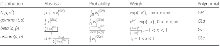
Nth degree and not necessarily be the integers. As such derived distribution is not discrete in the sense of having integer support. So this is rather a way of approximating a pdf fX(x) by a pmf {pj},j= 1, 2,…,MNwhich retain common moments and cdf value at the points of discretization. A list of approximation of some classical probability dis-tribution proposed by Luceno (1999) is given in Table 1 below:
The gamma (t,α) distribution has mean t/α and variance t/α2; the superscript Gauss-Hermite (GH), Gauss-Laguerre (GLa), Gauss-Jacobi (GJ) and Gauss-Legendre (GLe) refer to the polynomial names; the subscriptjvaries in {1, 2,…,N}.
This method may require solution of system of non-linear equations in addition to the requirement of the existence of moments of the continuous distribution.
2.8 Methodology-VIII
Hagmark (2008) presented a method for constructing nonnegative integer-valued ran-dom variables with any interval ran-domain, any theoretically possible mean–variance pair, and different shapes using basic tool of a mean preserving discretization method in which the discretization of a nonnegative initial random variableXwith cdfFX(x) is de-fined as the count variableYwith cdf
Table 1Approximation of some classical probability distribution
Distribution Abscissa Probability Weight Polynomial
N(μ,σ2) μþσxð ÞjGH 1ffiffi π
p wð ÞjGH exp(−x2),− ∞<x<∞ GH gamma(t,α) 1
αxðjGLaÞ Γ1tw
GLa
ð Þ
j xt−1
′
expð Þ−x;0<x<∞ GLa beta(α,β) ð1þxð ÞjGJÞ
2
t1−α−βwð ÞGJ j
betaðα;βÞ ð1−xÞ α−1
1þx
ð Þ1−β;−1<x<1 GJ
uniforn(a,b) aþ b−a
2 1þxðGLeÞ j
ð Þ 12w
GLe
ð Þ
FYð Þ ¼y P Yð ≤yÞ ¼ Zyþ1
y
FXð Þy dx
He has shown that under this construction
(i)E(X) =E(Y) and (ii)Var(X)≤Var(Y)≤Var(X) + min{E(X), 1/4}.
Note thatFY(y) is actually the average ofFX(.) in the interval (n,n+ 1) under assumption of uniform distribution in that interval. Hagmark (2008) asserted that every count variable is a discretization of an initial continuous random variable which is seldom unique. He gave example initial continuous distribution of which Poisson distribution is a discretized version and algorithms to generate discrete distributions using this method.
2.9 Two stage composite methods 2.9.1 Discretized Exponentiated models
In this method the discrete analogue of the continuous random variable X having cdf
FX(x) and sfSX(x) is derived as a discrete random variableYhaving pmf
P Yð ¼kÞ ¼SXð Þk α−SXðkþ1Þα;y¼0;1; 2;…;α>0
Thus basically first the continuous distribution function is exponentiated and the resulting exponentiated continuous distribution is then discretized by using the methodology-IV.
For example, by exponentiating the cdf of the continuous exponential distribution Gupta and Kundu (1999) derived generalized exponential distribution having pdf, cdf and sf
fxð Þ ¼x αλ1−e−λxα−1e−λx; x>0;α>0;λ>0:
FXð Þ ¼x 1−e−λx
α
and SXð Þ ¼x 1− 1−e−λx
α
respectively:
Writingq=e−λ, a discrete analogue of this distribution can be obtained with pmf
P Yð ¼kÞ ¼1−qkþ1α−1−qkα;k¼0;1;2;⋯ ð16Þ
Which is the distribution mentioned in Eq. (13) and again later in Eq. (20). (see Mudholkar
et al.(1995) for exponentiated Weibull).
Remark 1.One can use the exponentiation of sf and then discretize to get different
analogues. Also one can use other methodologies instead of method III to generate dif-ferent discrete analogues of the exponentiated continuous distributions.
2.9.2 Two-fold competing risk models
In this method (Jiang 2010) first two continuous random variablesX1andX2having sfs
SX1ð Þx and SX2ð Þx are combined to produce a new random variable X having sf
SXð Þ ¼x SX1ð ÞSx X2ð Þx:
Then a discrete analogueYofXis derived fromSX(x) by using methodology-IV. The resulting pmf is
P Yð ¼kÞ¼SXð Þk−SXðkþ1Þ ¼SX1ð Þk SX2ð Þk −SX1ðkþ1ÞSX2ðkþ1Þ
Where PXiðY ¼kÞ ¼SXið Þk −SXiðkþ1Þ is the discrete analogue of the continuous
random variableX1. Clearly, the random variableXis equal to minimum {X1,X2}. Discrete additive Weibull distribution discussed in the section 2.4.21 can be seen as an example of this construction.
Remark 2.
i. Obviously, one can generalize this to more than two i.e. manifold competing risk models model.
ii. Discretized exponentiated method can be seen as a particular case of this method when theX’s are identical.
2.9.3 Marshall and Olkin followed by method-III
In this method first the sf SX(x) of a continuous random variableX is generalized by adding an extra parameter αusing Marshall and Olkin (1997) scheme then discretize by using the methodology-IV. The generalized sf is then
SXðx;αÞ ¼ α
SXð Þx 1−ð1−αÞSXð Þx
ð17Þ
and the corresponding pmf of the discrete analogue by method-IV is
P Yð ¼kÞ ¼SXðk;αÞ−SXðkþ1;αÞ ¼ α
SXð Þ−Sk Xðkþ1Þ
f g
1−ð1−αÞSXð Þgk f1−ð1−αÞSXðkþ1Þg
f ð18Þ
2.9.3.1 Generalization of the geometric distribution Gómez-Déniz (2010) proposed
and studied a new generalization of the geometric distribution by using this scheme of discretization. They started with X following exponential distribution with sf SX(x) = exp(−θx) =qx, where q=e−λand used the construction in Eq. (18) generalize the geo-metric distribution with pmf
P Yð ¼kÞ ¼ αq
kð1−qÞ
1−ð1−αÞqkþ1gf1−ð1−αÞqkÞ
f g; k¼0;1;2;⋯
2.9.3.2 Discrete half normal Gómez-Dénizet al.(2014) proposed a discrete version of
the half-normal distribution by using this scheme of discretization and investigated its generalization with applications.
First takingSX(x) =ΦX(x) whereΦX(x) is the cdf ofN(0,σ) in Eq. (17) a generalization of the normal distribution is obtained with sf
SXð Þ ¼x α
1−ΦXð Þx
f g
1−ð1−αÞf1−ΦXð Þxg;−∞<x<∞
Then the sf for the corresponding distribution in R+ which can be considered as a generalization of thehalf-normaldistribution is given by
SXð Þx
SXð Þ0
¼ ð1þαÞf1−SXð Þxg 1−ð1−αÞf1−SXð Þx g;
Now employing the methodology-IV the pmf of discrete generalized half normal dis-tribution is obtained as
P Yð ¼kÞ ¼ ð1þαÞfΦXðkþ1Þ−ΦXð Þk g
1−ð1−αÞð1−ΦXð Þk Þgf1−ð1−αÞð1−ΦXðkþ1ÞÞg
f
In particular for α= 1, we get the discrete half normal distribution Chakraborty (2015a) with pmf
P Yð ¼kÞ ¼2½ΦXðkþ1Þ−ΦXð Þk
2.9.4 T-X method
Suppose FX(x), hX(x) and HX(x) =−log(1−FX(x)) be respectively the cdf, the hazard rate function and cumulative hazard rate function of any random variable X. fT(t) and
FT(t) be the pdf and cdf of another continuous random variableT defined on (0, ∞). The cdf of the random variableYhavingT-Xfamily of distributions defined by Alzaatreh
et al.(2012) is then given by
FYð Þ ¼y Z −log 1ð−FXð ÞyÞ
0
fTð Þdtt ¼FTf−log 1ð −FXð Þy Þg;
whenXis a continuous random variable the corresponding pdf of theT-Xfamily can be obtained as
fYð Þ ¼y fXð Þy
1−FXð Þy
fTð−log 1ð −FXð Þy ÞÞ ¼hXð Þy fTðHXð Þy Þ:
If X is a discrete random variable, the T-Xfamily is a family of discrete distribution transformed from thenon-negativecontinuous random variableT. The pmf of theT-X
family of discrete distribution can be found as
P Yð ¼kÞ ¼FYð Þ−Fk Yðk−1Þ
¼FTf−log 1ð −FXð Þk Þg−FTf−log 1ð −FXðk−1ÞÞg;k¼0; 1; 2; … ð 19Þ
As such we can see that this method is essentially employing discretization method on theT-Xpdf to generate new discrete distribution.
IfXis a geometric random variable with cdfFX(x) = 1−px+ 1,x= 0, 1, 2,…, thenT-X
family in Eq. (19) is referred to as theT-geometricfamily with pmf
¼FTf−log pkþ1
−FTf−log pk
¼FTf−ðkþ1Þlogpg−FTf−klogpg;k¼0; 1; 2; …
ð20Þ
In particular if X is a geometric random variable with parameter p=e−1= 0.3679, then pmf of theT-geometricfamily reduces toP(Y=k) =FT(k+ 1)−FT(k),k= 0, 1, 2,… (see section 2.5).
Alzaatrehet al.(2012) proved many properties of this family including the unimodal-ity of the T -geometricfamily given that the non-negative continuous random variable
Tis unimodal with a unique mode.
FTð Þ ¼t 1−e−λt
α
;t>0; α>0; λ>0
thenT-geometricfamily in Eq. (20) leads to theexponentiated exponential–geometric distribution (EEGD) with pmf
P Yð ¼kÞ ¼ 1−pλðkþ1Þ
α
−1−pλkα; k¼0; 1; 2; …: ð21Þ
On replacingpλbyθ, we will have
P Yð ¼kÞ ¼1−θkþ1α−1−θkα; 0<θ<1; k¼0; 1; 2; …:
Note that, if α= 1, i.e. the random variableT has exponential distribution, and then the EEGD reduces to the geometric distribution. Also observe the similarity of Eq. (21) with Eqs. in (13) and (16).
2.9.5 Generalization of the T-X method
LetfT(t) be the pdf of a continuous random variableT defined on [a,b] andW(.) be a absolutely continuous and monotonically non-decreasing function with W(0)→a and
W(1)→b. Then the cdf of the generalized T-X family of distributions defined by Alzaatrehet al.(2013) is given by
fYð Þ ¼y
Z W F yð ð ÞÞ
0
fTð Þdtt ¼FT½W Fð Xð Þy Þ;
If Xis a non-negative discrete random variable, then the pmf of this generalizedT-X
family of discrete distribution can be found as
P Yð ¼kÞ ¼FTfW Fð Xð Þk Þg−FTfW Fð Xðk−1ÞÞg;k¼0; 1; 2; … ð22Þ
Obviously Eq. (22) reduces to Eq. (19) whenW(x) =−log(1−x).
Akinsete et al. (2014) consideredTas the Kumaraswamy (1980) distribution with cdf
FT(t) = 1−(1−tα)β, 0 <t< 1,α> 0, β> 0, Xas the geometric random variable with cdf
FX(x) = 1−px+ 1,x= 0, 1, 2,…andW(x) =xin Eq. (21) to propose the Kumaraswamy-geometricdistribution with pmf
P Yð ¼kÞ ¼h1−1−pkαiβ−h1−1−pkþ1αiβ; k¼0; 1; 2; …: ð23Þ
Note that for β= 1, Eq. (23) reduces to Eq. (21). Akinseteet al. (2014) also proved that this distribution can also be derived by considering log-Kumararswamy distribu-tion instead of Kuamarswamy distribudistribu-tion and takingW(x) =−log(1−x).
2.9.6 Method of discretization after transmutation
Chakraborty (2015b) recently introduced the idea of discretization of transmuted continu-ous distributions. A random variable Z is said to be constructed by the quadratic rank transmutation map method of Shaw and Buckley (2007) by transmuting another random variableXwith cdfFX() if the cumulative distribution function (cdf ) ofZis given by
So given a cdf FX(x) of a continuous random variableX, it is first transmuted toFZ(z) by adding an extra parameterαusing Shaw and Buckley (2007) scheme then discretized by using the methodology-IV. The corresponding pmf of the new discrete distribution is then given by
P Yð ¼kÞ ¼ð1þαÞ½FXðkþ1Þ−FXð Þk −α ðFXðkþ1ÞÞ2−ðFXð Þk Þ2
For example consideringFX(x) = 1−βe−βx, the pdf and cdf of the transmuted exponential distribution derived using the quadratic rank transmutation by Shaw and Buckley (2007) are respectively given by
fZð Þ ¼z βe−βzð1−αÞ þ2αβe−2βz;z>0;β>0;−1<α<1
FZ(z) = (1 +α)(1−e−βz)−α(1−e−βz)2,z> 0,β> 0,−1 <α< 1 (Shaw and Buckley, 2007). Now using the methodology-IV the pmf of the discrete analogueYof transmuted ex-ponential, is obtained as
P Yð ¼kÞ ¼FZðkþ1Þ−FZð Þk
¼ð1−αÞqkð1−qÞ þαq2kð1−q2Þ;k¼0;1;2;⋯;0<q<1;−1<α<1
withe−β=q. This is the transmuted geometric distribution proposed recently by Chak-raborty (2015b) and studied in detail by ChakChak-raborty and Bhati (2015).
3. Discussion and conclusions
3.1. Benefits of discretization of continuous probability distribution
When only an approximating discrete random variable is observable, estimation proce-dures employing the hypothetical continuous random variables are sometime biased and hence a discrete distribution is more appropriate for an observed data (Holland 1975).
Discretization of continuous distribution may be looked upon as a filtering process which may help in reducing of noise present in the data. Especially data sets having a high amount of background noise can gain from this process.
Discretization may bring in computational easiness.
3.2 Limitation of discretization of continuous probability distribution
When a continuous probability density function is discretized to a probability mass function there will always be some loss of information. As such one should try to strike a balance between the need for discretization and resulting loss of information or ac-curacy. Also attention should be paid to select the best one among the available tech-niques of discretization. Some of the criteria for selection mentioned in Bracquemond and Gaudoin (2003) are simple and flexible expressions, physical basis for the distribu-tion, interpretation of model parameter, and efficiency of estimators.
3.3 Concluding remarks
vibrant research topic. Future research in this area may be to search for different constructions that might ensure preservation of multiple characteristics of the con-tinuous distribution in its discretized version, developing inferential procedures for these discrete analogues etc. among others. We have not discussed detail properties of the methods and discretized distributions presented in this survey as those can accessed from the respective original references.
Competing interests
The author declares that he has no competing interests. Authors’contributions
The author contribution is sole. Acknowledgement
Author would like to acknowledge the remarks and suggestions made by various research scholars and scientists in theInternational Conference on Statistical Data Mining for Bioinformatics, Health, Agriculture and Environment, at Rajshahi University, Bangladeshduring December 22−24, 2012 where an earlier version of this paper was first presented as an Invited talk.
Author would also like to acknowledge the anonymous referee and editor for their comments and suggestions on the first draft of this paper which lead to substantial improvements in presentation.
Received: 4 February 2015 Accepted: 1 July 2015
References
Akinsete, A, Famoye, F, Lee, C: The Kumaraswamy-Geometric distribution. J. Stat. Distributions. Appl.1, 17 (2014) Alhazzani, NS: Modeling discrete life data in reliability and its applications. Master thesis. King Saud University, Riyadh (2012) Al-Huniti, AA, AL-Dayian, GR: Discrete Burr type III distribution. Am. J. Math. Stat.2(5), 145–152 (2012). doi:10.5923/
j.ajms.20120205.07
Almalki, SJ: Statistical analysis of lifetime data using new modified Weibull distributions, a thesis submitted to the University of Manchester for the degree of Doctor of Philosophy in the Faculty of Engineering and Physical Sciences. (2014)
Almalki, SJ, Nadarajah, S: A new discrete modified Weibull distribution. IEEE. Trans. Reliability.63(1), 66–180 (2014). doi:10.1109/TR.2014.2299691
Al-Masoud, TA: A discrete general class of continuous distributions. Master of Science (Statistics) thesis. Faculty of Science, King Abdul Aziz University, Jeddah-Saudi Arabia (2013)
Alzaatreh, A, Lee, C, Famoye, F: On the discrete analogue of continuous distributions. Stat. Methodol9, 589–603 (2012) Alzaatreh, A, Lee, C, Famoye, F: A new method for generating families of continuous distributions. Metron71, 63–79 (2013) Bakouch, HS, Jazi, MA, Nadarajah, S: A new discrete distribution. Statistics,iFirst,1-41 (2012). doi/10.1080/
02331888.2012.716677
Barbiero, A: A discretizing method for reliability computation in complex stress-strength models. World. Acad. Sci. Eng. Technol.47, 75–81 (2010)
Barbiero, A: An Alternative discrete skew Laplace distribution. Stat. Methodol16, 47–67 (2014)
Barbiero, A: Parameter estimation for type III discrete Weibull distribution: a comparative study. J. Probab. Stat., Volume 2013, Article ID 946562, http://dx.doi.org/10.1155/2013/946562
Bebbington, M, Lai, CD, Wellington, M, Zitikis, R: The discrete additive Weibull distribution: a bathtub shaped hazard for discontinuous failure data. Reliability Engineering and System Safety (2012)
Benkherouf, L, Bather, JA: Oil exploration: sequential decisions in the face of uncertainty. J. Appl. Probability.25, 529–543 (1988)
Bi, Z, Faloutsos, C, Korn, F: The“DGX”distribution for mining massive skewed data. 7th Conf. on Knowledge discovery and data Mining, San Francisco (2001)
Bracquemond, C, Gaudoin, O: A survey on discrete life time distributions. Int. J. Reliabil. Qual. Saf. Eng.10, 69–98 (2003) Byers, Jr, RH, Shenton, LR: Surprising approximations to the half-normal. Journal of Statistical Computation and
Simulation49(3), 215–216 (1994)
Carver, HC: On the graduation of frequency distributions. Proc. Casual. Actuarial. Soc. Am.6, 52–72 (1919) Carver, HC: Frequency curves. Handbook of Mathematical Statistics. Rietz, HL (editor), Cambridge MA: Riverside, 92-119 (1923) Chakraborty, S: A new discrete distribution related to generalized gamma distribution and its properties. Commun. Stat.
Theory. Methods.44(8), 1691–1705 (2015). doi:10.1080/03610926.2013.781635
Chakraborty, S, Chakravarty, D: Discrete gamma distributions: properties and parameter estimation. Commun. Stat. Theory. Methods.41(18), 3301–3324 (2012)
Chakraborty, S, Chakravarty, D: A discrete Gumbel distribution. arXiv:1410.7568 [math.ST], 28 Oct 2014 Chakraborty, S, Chakravarty, D: A discrete two sided power distribution. arXiv:1501.06299[math.ST], 26 Jan 2015 Chakraborty, S, Chakravarty, D: A new symmetric discrete probability distribution with integer support on (-∞,∞).
Published on line 12thAugust 2013, Communications in Statistics-Theory and Methods (2013)
Chakraborty, S, Gupta, RD: Exponentiated geometric distribution: another generalization of geometric distribution. Commun. Stat. Theory. Methods.44(6), 1143–1157 (2015). doi:10.1080/03610926.2012.763090