http://www.sciencepublishinggroup.com/j/ajnna doi: 10.11648/j.ajnna.20180401.13
ISSN: 2469-7400 (Print); ISSN: 2469-7419 (Online)
An Effective Combination of Pre-Processing Technique and
Deep Learning Algorithm for Hammering Sound Inspection
Balage Don Hiroshan Lakmal, Daisuke Oka, Yoichi Shiraishi, Kazuhiro Motegi
Department of Science and Engineering, Graduate School of Science and Technology, Gunma University, Gunma, Japan
Email address:
To cite this article:
Balage Don Hiroshan Lakmal, Daisuke Oka, Yoichi Shiraishi, Kazuhiro Motegi. An Effective Combination of Pre-Processing Technique and Deep Learning Algorithm for Hammering Sound Inspection. American Journal of Neural Networks and Applications.
Vol. 4, No. 1, 2018, pp. 15-23. doi: 10.11648/j.ajnna.20180401.13
Received: July 3, 2018; Accepted: August 6, 2018; Published: September DD, 2018
Abstract:
This paper deals with the identification problem of defective products of door strikers installed in automobiles based on their hammering sounds. The difference of the hammering sounds between defective and acceptable products is very small and each sound signal has a unique pattern. The capabilities of conventional human sensory tests are not enough to identify such differences between these two classes. Hence it is suggested to apply deep learning algorithms (DLA) as per the versatility and feature extraction power. Usually, some kinds of pre-processing are adopted before the application of DLA in order to increase the accuracy of inspection as well as to reduce the training and the application time of DLA. In this paper, the combinations of five kinds of pre-processing techniques and three types of DLAs are applied to the actual hammering sounds inspection of door strikers. Especially in two types of DLAs, the sound data have been evaluated as images. The evaluation results show that the combination of the wavelet analysis and the Convolutional Neural Network (CNN) only attained the 100% accuracy of inspection with great response time. The wavelet analysis and the CNN are independently attain the high performances comparing with others and it is likely that they are useful in this kind of hammering sound inspections.Keywords:
Pre-Processing, Deep Learning Algorithms, Non-Destructive Testing, Door Striker, Convolutional Neural Network, Wavelet Analysis1. Introduction
Currently, many industrial quality control inspections are based on non-destructive inspection methods and conventional approaches are carried on to identify the testing pattern by human, co-called a human sensory test. In many cases, sound waves have been considered as a media for Quality Analysis (QA) or Quality Control (QC) activities because of their various features or properties such as frequency, wavelength, amplitudes, wave speeds, intensities, timbres and directions can be considered for any kind of analysis.
In this research, hammering sounds are considered as input media. The hammering sound inspection is strongly dependent on human experts’ experiences. Additionally the processing time is also a crucial factor to keep the production rate efficient. Moreover, the inspection process may be getting worse with the presence of environmental noise or the
non-hammering sounds. Because of the industrial applications, if even a single defected piece passes through the inspection process, such an inspection system would not be practical.
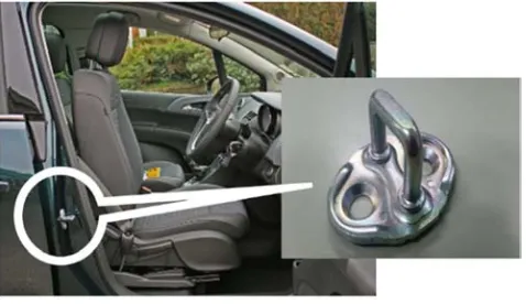
Figure 1. Automobile door striker.
The configuration of this paper is as follows. In Chapter 2, some current approaches in the hammering sound inspection are shown. Chapter 3 is assigned to the description of proposed approach. Here, the combinations of pre-processing and DLA`s are suggested. The experimental results are reported in Chapter 4 and the best combination of PPT and DLA is shown. Finally, this paper is concluded in Chapter 5.
2. Current Approaches
The same research [1] is performed by using Support Vector Machine (SVM) and the supervised learning approach uses to solve the door striker inspection problem. The advantage of this approach is its speed in both of the learning and the judgement processes. In this research, the hammering sound has firstly transformed to the spectrum distribution by using Fast Fourier Transform (FFT) and then, the spectrum distribution is an input to the SVM. This approach attained the good quality in some experiments, actually, 95.2%, however, the practical level performance has not yet been attained because both of 100% detection rate and 100% accuracy rate are indispensable in the product inspection. Actually, the typical defected sample can be properly excluded, however, such defected samples as difficult to detect are not recognized in this approach.
The hammering sound inspection is generally much more difficult than the appearance inspection because the hammering sound is very sensitive to the recording environments and noises. Up to now, as two types of hammering sound inspection methods, off-line and on-line, several papers are published. The off-line hammering sound inspection means that the collected data will be checked without any limit of time. For example, the hammering sounds are all recorded at field sites and then, those data are analyzed and checked in the laboratory or office. They are mainly applied to various kinds of artifacts [2, 3, 4, 5, 6]. However, the accuracy of inspection is not necessarily sufficient even if human experiences are utilized. Moreover, as for the on-line hammering sound inspection, only an automatic crack detector for eggs [7] is commercially available, however, its accuracy is still 95%.
In regardless of hammering sound, EEG signal classification researches also have shown much better results [8, 9, 10]. But such a medical applications, time is not a crucial
factor compared to a production line.
3. Proposed Approach
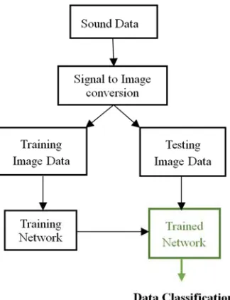
In this application, a combination of DLA and Pre-Processing Technique (PPT) which shows optimum performance is proposed for the signal data classification after analyzing different combinations as shown in Figure 2.
In this research flow, the recorded sound data are put into the classification process. The classification process consists of all combinations of five PPTs and three DLAs. The details of these PPTs and DLAs are described in the followings and the best combination is determined against the actual hammering sounds of door strikers.
Figure 1. Research flow chart.
3.1. Hammering Sound Inspection System
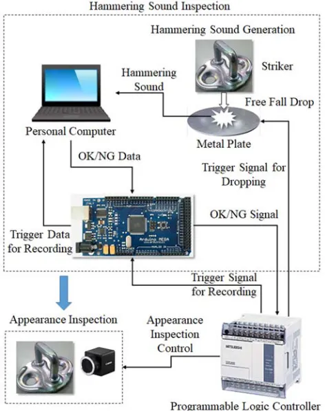
The sound inspection system dealt with in this research is shown in Figure 3. This system consists of hammering sound inspection and the appearance inspection which are controlled by the Programmable Logic Controller (PLC).
Figure 3. Hammering sound inspection system.
3.2. Data Pre-Processing
The output of DLA always not only depends on its design and performance but also very dependent on the quality and suitability of input sound signals. Hence, the input sound signals having negative factors such as noise, missing values, inconsistent and superfluous data highly influence the feature extraction and classification. With this scenario, the input signal data is subjected to various PPTs to increase the output accuracy despite of having high power of different feature extracting methods for the data classification. Following PPTs have generated a good detailed discrete signals.
3.2.1. Short Term Energy Analysis (STEA)
The total energy of a signal can be expressed as in (1).
∑ . (1)
Here, n is the shift / ratio in number of samples at which we are interested in knowing the short term energy. W represent the windowing function of finite duration and S is the discrete signal.
3.2.2. Wavelet Analysis (WA)
The WA uses filters of different cutoff frequencies to analyze the signal at different scales. As shown in Figure 4 (a), the signal X [n] is passed through a high pass filter H to analyze the high frequencies by removing low frequencies and low pass filter G to analyze the low frequencies by removing high frequencies. The output of G is called wavelet approximation coefficient and the output of H is called the
wavelet detailed coefficient. The process is continued to decompose the signal to a pre-defined certain level. This operation is called decomposition.
After the decomposition is completed as per the predefined level, then the signal reconstruction process is continued as shown in Figure 4 (b). Basically, the reconstruction is the reverse process of decomposition. The approximation coefficient and detailed coefficients at every level passed through the low pass and high pass filters G'and H' then added. This process is continued through the same number of levels as in the decomposition process to obtain the original signal approximation X'[n]. The H, H', G and G' were defined as per the selected wavelet. In this research Sym 4 wavelet was used for the above analysis. [11].
(a) Wavelet decomposition
(b) Wavelet reconstruction
Figure 4. Level 3 wavelet analysis.
3.2.3. Cross- Correlation (CC)
This is a standard method of estimating the degree to which two series are correlated. Consider two series X (i) and Y (i) where i = 0, 1, 2,..., N-1. The cross correlation r at delay k can be defined as (2) [12].
∑
∑ ∑ (2)
Here, ∑! ! & " ∑ "! !
3.2.4. Fast Fourier Transform (FFT)
X (s) ∑ # $ %(' ) !⍵' (3) 3.2.5. Discrete Walsh-Hadamard Transform (DWHT)
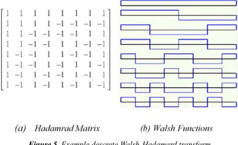
Walsh–Hadamard transforms are also known as Walsh or Walsh-Fourier transforms. This is an orthogonal transformation that decomposes a signal into a set of orthogonal, rectangular waveforms called Walsh functions as shown in Figure 5. In here, each row of the Hadamard matrix (Figure 5 (a)) represents a unique Walsh function (figure 5 (b)) and hence the number of Walsh functions are equal to the number of rows in Hadamard Matrix [14].
Figure 5. Example descrete Walsh-Hadamard transform.
Forward Walsh-Hadamard Transform yn of signal xt with length n can be expressed as (4). Here, WALn,i is the Walsh function with length N.
* (∑(! ) #!+,- ,! (4)
3.3. Overview of DLA
DLA can be defined as a Neural Network architecture facilitating deep learning, retrieval and analysis of data that are deeply buried in input information and otherwise not easily retrievable. Their ability to dig deeply in the input data is often superior and/or faster to other non-neural network computational methods due to their efficient integration of mathematical, logical and computational methods. The network consists of nodes or units connected by links. Each link has a numeric weight associated with it. The weights are the primary means of long-term storage in neural networks and the learning usually takes place by updating the weights.
The error function E shown in (5) is calculated as per the gradient descent method with mean square error starting from random weights. Here, O is predicted output and T is correct output.
E = ||0 – 2|| (5)
The gradient of the error function E can be expressed as in (6).
3 E=5756 (6)
Then the updated weight ! 87 from the previous weight
!9:; can be defined as in (7).
! 87= !9:;
ή
∙3 (7)Here ή represent the learning rate of the iteration [15, 16, 17].
The backpropagation is normally used for network learning which consists of three main operations such that forward pass, backward pass and weight update. Then the new weight value is used to generate new output. These processes are continued until the error function reaches the global minimum.
It is important to understand the difference between the supervised learning and the unsupervised learning network behavior. In the supervised learning, input and output pairs (Target) have to be fed in to the network. In contrast, unsupervised learning the same input is treated as a target. As per the output of each network, the error function can be defined. In this research, there are three types of network which are subjected for the classification.
3.3.1. Feed Forward Network (FFN)
An FFN consists of input layer, {x1, x2, x3, …, xn}, single hidden layer, {f1, f2, f3, …, f30} and output layer Y as shown in Figure 6. The performance of the network varies with the number of neurons in hidden layer. Here, 30 number of neurons ae included in the hidden layer for the classification. This network is trained under the supervised learning method. Hence the target and input pair has to be fed in to the network during the training.
Figure 6. Two layered FFN.
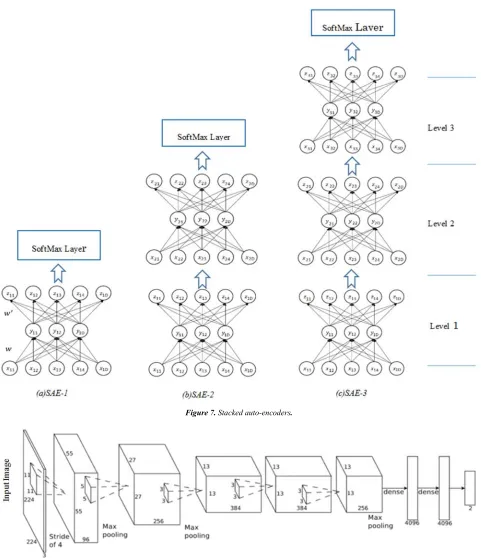
3.3.2. Stacked Auto Encoder (SAE)
Auto-encoders are simple learning circuits which used to regenerate the signal with the least possible amount of deformation. The Deep Neural Networks (DNN) are implemented in three ways by stacking single, 2 and 3 auto-encoders such as SAE-1, SAE-2 and SAE-3, respectively shown in Figure 7. Following equation can be expressed with ƒ and g, where, f is the function from the input layer to the hidden layer and g is the function from the hidden layer to the output layer. Hence, the output of each layer can be expressed as (8).
=
g(Y)
g∙ƒ
X
, (8)
where, Y ƒ X.
function ! defined in (9).
! @ ∑ ∆! g ∙ ƒ #!, , #!, (9) Here, ∆ is the dissimilarity between the output vector and the input vector [18].
3.3.3. Convolutional Neural Network (CNN)
The CNN consists of complex structure as shown in Figure
8. In this research, the pre-trained network model designed by Alex, Ilya and Geoffrey in University of Toronto [19], is used for the classification. Basically CNN is used for image classification by extracting its features. The image passes through different kind of layers, each having specific operation with input the signal image.
Figure 7. Stacked auto-encoders.
The network consists of 25 layers. The convolutional layer, the pooling layer and the Rectified Linear Unit (RELU) layers are fully connected repeatedly. The convolutional layer generates the key operation such that the input image is convoluted with learnable kernels (K) and generates a new feature map (FM) for specific kernel as per (10). The projection of kernel into input image is called the Receptive Field (RF) [20].
FM=∑L )9:K I∑H97IJ ) CD # E, * F G #, * (10)
3.4. Input Data Structure
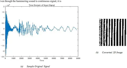
Even though the hammering sound is continuous signal, it is
copied into the system and then signal becomes a discrete form such that the x axis represents a small time interval and the y axis represents the amplitude of the sound. Therefore, the signal can be represented as a 1D matrix array. This data form is not changing while PPTs are applied.
For FFN, the data can be fed in to the network as its original 1D matrix form. However, for CNN and SAE, the data need to be converted into the 2D images before fed into the network. The 1D matrix array is then converted into the 2D matrix by specifying correct dimension to fit each element of the 2D matrix as shown in Figure 9. Then the combinations of five PPTs and three DLA are suggested as shown in Figure 10.
Figure 9. 2D image conversion of hammering sound. The size of original signal was adjusted to generate square 2D image as shown in (b).
Figure 10. Suggested combinations of PPTs and DLAs.
Each element of the above matrix determines the intensity of the corresponding pixel. Especially in a gray scale image, each element of the matrix is fixed between the specific integer numbers, 0 and 255. Specifically 0 represents the minimal intensity as a black pixel and the integer 255 represents a maximum intensity as a white pixel. The value of element in the matrix higher than 255 gives a white pixel and
lower than 0 gives a black pixel. Then, after the conversion of original hammering sound wave signal into 2D image as shown in Figure 9 (b), the grayscale image with the element values between 0 and 255 are generated.
Figure 11. Image training flow chart.
4. Experimental Results
Three types of datasets used in the experiments are as per Table 1. They are actually obtained in the hammering sound inspection system shown in Figure 3 based on the same way as that in the factory.
Table 1. Datasets used in experiments.
Datasets Acceptable Samples Defective Samples Total
Dataset 1 269 145 414
Dataset 2 500 500 1000
Dataset 3 3000 1950 4950
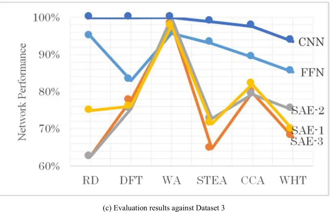
Three datasets with five kinds of PPTs along with raw dataset are applied to three DLAs which generated totally fifty four (3x6x3) of system outputs to identify best combination showing the highest system accuracy. The applications are performed by using MATLAB R2016b with Neural Network Toolbox, Parallel Computing Toolbox™ with CUDA®-enabled NVIDIA® GPU with compute capability 5.
(a) Evaluation results against Dataset 1
(c) Evaluation results against Dataset 3
Figure 12. Comparisons of accuracies of combinations of PPTs and DLAs.
By analyzing accuracy curves shown in Figure 12, CNN shows the best results with 64.2% minimum performance and only this network gives 100% maximum accuracy for all datasets with WA conversion. Meanwhile DS-3 shows maximum results having 97.56% minimum and 100% maximum. With all of these factors, CNN shows promising results than other DLAs. By considering all the results gained so far, following facts can be highlighted.
The accuracy always changed with key factors such as the network architecture, the learning rate, number of hidden layers, training algorithm, number of iterations etc., and can be defined as per the user. However, every DLA is used to be trained several times until showing better accuracy and this is a common practice.
For the DNN training, large training dataset should be needed to increase the performance which may cause to delay the process to some extent. Overfitting is a key aspects to be happened in the DLA training that leads to decrease the accuracy of testing samples while showing great accuracy in training samples.
The main drawback is that the internal operation of DNN cannot be determined. Once the network trained and if the given output is beyond the expected level, then the reason is really difficult to predict what leads to the lack of confidence of the network output. This is one of our future research themes.
Overall, it is shown that each dataset transformed with WA generates best results with CNN based on the observations showing 100% data classification accuracy.
5. Conclusion
This paper deals with the problem what combinations of pre-processes and deep learning algorithms give the best performances by using the actual hammering sound inspection problem. Five kinds of such pre-processes as Short Term Energy Analysis, Wavelet Analysis,
Cross-Correlation, Fast Fourier Transform and Discrete Walsh-Hadamard Transform are adopted. As deep learning algorithms, Feed Forward Network, Stacked Auto Encoder, and Convolutional Neural Network are used. The experimental results show that only the combination of Wavelet Analysis and Convolutional Neural Network attains 100% accuracy against three datasets consisting of actual hammering sounds. Moreover, it is concluded that Convolutional Neural Network attains the highest accuracy among deep learning algorithms and also Wavelet Analysis is the best among pre-processes. As future work, the detailed processes inside of deep learning algorithms should be analyzed, the incremental learning should be researched and the hammering sound inspection system implementing the obtained best combination is should be in practical use as soon as possible. Moreover, it is expected that other DLA application areas of the combinations dealt with in this paper would be investigated.
References
[1] Daisuke Oka, Don Hiroshan Lakmal Balage, Kazuhiro Motegi, Yasuhiro Kobayashi, and Yoichi Shiraishi, “A Combination of Support Vector Machine and Heuristics in On-line Non-Destructive Inspection System,” International Conference on Machine Learning and Machine Intellignece (MLMI), Hanoi, Vietnam, September, 2018 (In press).
[2] Tetsuharu Akiyama, Satoshi Kiyomiya, Yuta Yamashita and Naoyuki Iki, “An Analytical Consideration of Hammering Sound Method as Nondestructive Inspection Method," Proceedings of the Japan Concrete Institute, Vol. 26, No. 1, pp. 1815-1820, 2004.
[4] Keiichi Itohira, Hiromi Yamamoto, Keiichiro Yamamoto, Yasuhiko Wakibe, Mikio Iwamoto, Kenichi Yoshinaga and Takaki Egashira, " Hammering Inspection of the Soldering Part,” Research Report of Fukuoka Industrial Technology Center, No. 24, pp. 20-21, 2014.
[5] Atsushi Yamashita, Takahiro Hara and Toru Kaneko, “Hammering Test with Image and Sound Signal Processing,” Transactions of the JSME C, Vol. 72, No. 715, pp. 772-779, 2006.
[6] Shuji Takahashi, Masaya Miyajima, Atsushi Horiguchi, Kyoji Nakajo, Kazuhiro Motegi and Takashi Suda, “A Non-Destructive Defect Estimation of Metal Pole by using Hammering Sounds based on Machine Learning,” NAIS Journal, Vol. 10, pp. 9-15, September 2016.
[7] Grader: CANOPUS, NABEL Co., Ltd., Retrieved from https://www.nabel.co.jp/english/product/canopus.html. [8] B. Richhariya, M. Tanveer, “EEG signal classification using
universum support vector machine,” Expert Systems with Applications, Elsevier Journal, Volume 106, pp. 169-182, 2018.
[9] Sandeep Kumar Satapathya, Satchidananda Dehurib, Alok Kumar Jagadevc, “EEG signal classification using PSO trained RBF neural network for epilepsy identification,” Elsevier Journal, Informatics in Medicine Unlocked, pp. 1-11, 2017. [10] Manjeevan Seera, Chee Peng Lim, Kay Sin Tan, Wei Shiung
Liew, “Classification of transcranial Doppler signals using individual and ensemble recurrent neural networks,” Elsevier Journal, Neurocomputing pp. 337–344, 2017.
[11] Babatunde S. Emmanuel, “Discrete wavelet mathematical transformation method for non-stationary heart sounds signal analysis,” ARPN Journal of Engineering and applied science, vol. 7, pp. 1022-1026, August 2012.
[12] Paul Bourke, “Cross correlation,” (August 1996), Retrieved from http://paulbourke.net/miscellaneous/correlate/.
[13] “The discrete fourier transform,” pp82-pp85, Retrieved from http://www.robots.ox.ac.uk/~sjrob/Teaching/SP/l7.pdf. [14] Jennifer Seberry, Mieko Yamada, “Hadamard matrices,
sequences and block designs, Contemporary design theory – A Collection of Surveys,”D. J. Stinson and J. Dinitz, Eds., John Wiley and Sons, pp. 431-433, 1992.
[15] R. Rojas, “Neural networks,” Springer-Verlag, Berlin, Chapter 4/Chapter 7, pp. 77-83/, pp. 151-171, 1996.
[16] Danie Graupe, “Deep learning neural networks- Design and case studies,” World scientific publishing Co. Ltd., Chapter 5, pp. 41-53, 2016.
[17] Stuart Russell, Peter Norvig, “Artificial intelligence – A modern approach,”3rd ed., Prentice hall series in artificial intelligence, Chapter 19, pp. 563-597, 1995.
[18] Pierre Baldi, “Autoencoders, Unsupervised Learning, and Deep Architectures,” JMLR: Workshop and conference proceedings, pp. 27-37, 2012.
[19] Alex K., Ilya S., Geoffrey E., “ImageNet Classification with Deep Convolutional Neural Networks”, Communications of the ACM, Vol. 60, No. 6, pp 84-90, 2017.
[20] “Backpropagation In Convolutional Neural Networks,”
Retrieved from