www.adv-stat-clim-meteorol-oceanogr.net/2/17/2016/ doi:10.5194/ascmo-2-17-2016
© Author(s) 2016. CC Attribution 3.0 License.
Building a traceable climate model hierarchy with
multi-level emulators
Giang T. Tran1, Kevin I. C. Oliver1, András Sóbester2, David J. J. Toal2, Philip B. Holden3, Robert Marsh1, Peter Challenor1,4, and Neil R. Edwards3
1Ocean and Earth Science, National Oceanography Centre Southampton, University of Southampton, Southampton, UK
2Faculty of Engineering and the Environment, University of Southampton, Southampton, UK 3Environment, Earth and Ecosystems, Open University, Milton Keynes, UK
4College of Engineering, Mathematics and Physical Sciences, University of Exeter, Exeter, UK
Correspondence to: Giang T. Tran ([email protected])
Received: 1 September 2014 – Revised: 2 March 2016 – Accepted: 25 March 2016 – Published: 18 April 2016
Abstract. To study climate change on multi-millennial timescales or to explore a model’s parameter space,
efficient models with simplified and parameterised processes are required. However, the reduction in explicitly modelled processes can lead to underestimation of some atmospheric responses that are essential to the under-standing of the climate system. While more complex general circulations are available and capable of simulating a more realistic climate, they are too computationally intensive for these purposes. In this work, we propose a multi-level Gaussian emulation technique to efficiently estimate the outputs of steady-state simulations of an expensive atmospheric model in response to changes in boundary forcing. The link between a computationally expensive atmospheric model, PLASIM (Planet Simulator), and a cheaper model, EMBM (energy–moisture bal-ance model), is established through the common boundary condition specified by an ocean model, allowing for information to be propagated from one to the other. This technique allows PLASIM emulators to be built at a low cost. The method is first demonstrated by emulating a scalar summary quantity, the global mean surface air temperature. It is then employed to emulate the dimensionally reduced 2-D surface air temperature field. Even though the two atmospheric models chosen are structurally unrelated, Gaussian process emulators of PLASIM atmospheric variables are successfully constructed using EMBM as a fast approximation. With the extra infor-mation gained from the cheap model, the multi-level emulator of PLASIM’s 2-D surface air temperature field is built using only one-third the amount of expensive data required by the normal single-level technique. The con-structed emulator is shown to capture 93.2 % of the variance across the validation ensemble, with the averaged RMSE of 1.33◦C. Using the method proposed, quantities from PLASIM can be constructed and used to study the effects introduced by PLASIM’s atmosphere.
1 Introduction
Complex computer simulations are used in climate research to improve our understanding of the climate system. They are often used to project future changes in global tempera-ture, corresponding to different emission scenarios. Our con-fidence in these projections is highly dependent on how re-liable the simulations are. For example, the study of palaeo-climate offers an insight into the Earth’s past palaeo-climate system and also provides valuable out-of-sample data to validate our
achieved by a combination of lower spatial and/or temporal resolution and the use of simplified parameterisations. How-ever, depending on the nature of the questions asked, these lower fidelity models might be insufficient.
To address this issue, an emulator is often employed to provide a statistical estimation of the expensive model’s re-sponse without the need to perform a new simulation. Even then, this approach becomes impractical when the models of interest are very computationally intensive. In order to build a reliable emulator, a certain number of simulations is needed to provide the basis upon which the emulator is built. This number can be large, especially when multiple model pa-rameters are varied or when the model’s climate response exhibits non-linear behaviours. For a computationally expen-sive GCM, a sufficient number of simulations are often not affordable. This paper describes an efficient emulation pro-cess that utilises the connection between models of different complexities. The idea is to establish a traceable hierarchy, using an emulator for the simple model to construct an emu-lator of the more complex one (Kennedy and O’Hagan, 2000; Cumming and Goldstein, 2008).
While the high-fidelity (complex) model is computation-ally expensive, the low-fidelity (simple) model is cheaper to evaluate and can be sampled more finely across the in-put space, providing extra information where expensive data are sparse. The models forming this hierarchy can be struc-turally related or strucstruc-turally unrelated. Models are referred to as structurally related when they are from the same family of code but have different resolutions. These models might have other differences resulting from the change in mesh res-olution. Examples of such models are the HadCM3 (Hadley Centre Coupled Model version 3) (Pope et al., 2000) and FA-MOUS (Fast Met Office/U.K. Universities Simulator) (Jones et al., 2005) of the MET Office. Multi-level emulation has been employed before to link such models (Forrester et al., 2007; Cumming and Goldstein, 2008; Williamson et al., 2012). Here, our focus is on structurally unrelated atmo-spheric models, which solve different sets of equations. Since both the cheap and expensive codes model the same physical system, it is reasonable to expect qualitative similarities be-tween the two. This argument is supported by studies show-ing no systematic difference in model behaviour between EMICs and AOGCMs (Stouffer et al., 2006; Plattner et al., 2008; Zickfeld et al., 2013).
The following work illustrates the use of a method that combines multi-level emulation with a dimensional reduc-tion technique through an example study using GENIE-1, from the Grid ENabled Integrated Earth system mod-elling framework (GENIE), and PLASIM (Planet Simula-tor). GENIE-1 and PLASIM are chosen in this case since they are both suitable for Earth system modelling for long timescales, but are structurally different. PLASIM’s atmo-sphere is also substantially more complex and thus, compu-tationally more expensive than GENIE-1’s energy–moisture balance model, EMBM, of the atmosphere. EMBM
incorpo-rates the vertically integrated energy–moisture balance tions while PLASIM is based on the moist primitive equa-tions representing the conservation of momentum, mass and energy. EMBM, therefore, is not capable of producing air temperature and pressure at different altitude or an interac-tive cloud and wind field. The hierarchy formed by these two models is exploited using the multi-level technique, allowing us to construct an emulator of PLASIM atmospheric vari-ables at a reduced cost. Specifically, Gaussian process emu-lators are used to obtain the statistical relationship between the response of the EMBM atmosphere and the PLASIM at-mosphere to changes in their boundary conditions (sea sur-face temperature, long-wave and shortwave radiative forc-ing). This ability of this relationship to predict behaviour of PLASIM atmosphere, in the absence of feedbacks on other climate system components, is then assessed. The dimen-sional reduction technique is employed to extend the emu-lation method for prediction of high-dimensional outputs in addition to scalar summary quantities.
Once constructed, the emulators provide estimates of sim-ulation results, at untried combinations of the inputs, as finely as needed, at a low cost. This enables statistical methods such as history matching (Holden et al., 2010; Edwards et al., 2011) and sensitivity/uncertainty analysis (Rougier et al., 2009). Information from the cheap code can also be used to inform future designs of experiments using the expensive code. Apart from above, the emulators of 2-D surface fields similar to the one constructed here can potentially be used to provide the fields needed for coupling with other climate models or components of climate models.
2 Model configurations
In this study, we utilise the atmospheric component of GENIE-1 (version 2.7.8) (Lenton et al., 2006), an EMIC, as the cheap model. GENIE-1 was originally known as C-GOLDSTEIN in Edwards and Marsh (2005) and has since been modified for incorporation into the GENIE framework (Lenton et al., 2006). It is most recently described in Marsh et al. (2011). GENIE-1 is designed with scalable spatial reso-lution and high efficiency, suitable for long integrations (103 to 106 years) to study past climate and large ensembles to explore the uncertain input parameter space (Holden et al., 2010).
ef-fect of orography is applied to surface processes in ENTS by applying a constant lapse rate (Holden et al., 2010). Orogra-phy, therefore has an effect on the land surface temperature and so indirectly influences the atmosphere. The atmospheric processes such as heat and moisture transport do not interact with the orography.
The parameterisation of atmospheric transport of heat and moisture in EMBM is done by diffusion. Moisture can also be advected by a prescribed monthly climatological wind field. This wind field is fixed and is the same for all simula-tions in EMBM. The effect of cloud cover on incoming short-wave radiation is captured through a prescribed albedo field, diagnosed from reanalysis data (Lenton et al., 2006). The ef-fect of cloud cover on outgoing long-wave radiation is pa-rameterised as perturbations to the unmodified “clear-skies” outgoing long-wave radiation. Precipitation is assumed to oc-cur whenever the relative humidity is above a certain ad-justable threshold.
The atmosphere of PLASIM–ENTS (Holden et al., 2014), driven by boundary conditions specified by GOLDSTEIN ocean and sea ice, is chosen as the expensive model. PLASIM (Fraedrich et al., 2005) consists of an atmospheric GCM of intermediate complexity, which can interact with reduced sub-models of ocean, sea ice and land (Fraedrich et al., 2005). Hereafter, we refer to the atmospheric com-ponent of PLASIM–ENTS as simply PLASIM. PLASIM solves the primitive equations for vorticity, divergence, tem-perature and the logarithm of surface pressure. It includes a hydrological cycle, interactive clouds, and a simple radi-ation scheme. Coupling between the PLASIM atmosphere and an ocean model other than its own has been used before to study the effects of mountains and ice sheets on ocean cir-culation (Schmittner et al., 2011). An emulator of PLASIM– ENTS has been employed in a range of integrated assessment modelling couplings with various technico-economic models (Labriet et al., 2015; Mercure et al., 2014).
PLASIM is run at T21 resolution, which corresponds to a triangular truncation applied at wave number 21. It is almost an exact match of GENIE-1’s 64×32 mesh except for neg-ligible differences at the highest latitudes. While EMBM has only one layer, the atmosphere of PLASIM is represented by 10 vertical layers in terrain following σ-coordinates. Most importantly, EMBM uses prescribed wind fields, which means that feedbacks due to changing atmospheric circula-tion patterns are not captured, while PLASIM’s interactive wind field can change according to the different specified boundary conditions, leading to more diverse climate states. While the cloud albedo in EMBM is prescribed, the cloud albedo in PLASIM is a function of height and area of cover-age.
For our study, surface output fields of GENIE-1, namely, sea surface temperature (SST), fractional sea-ice coverage (SIC) and sea-ice thickness (SIH) are used to drive PLASIM. This means that the atmospheric circulation can change ac-cording to the underlying sea surface temperature and sea-ice
condition but cannot influence the ocean or sea-ice physi-cal state. This constrains PLASIM responses to a certain ex-tent. The atmospheric responses of EMBM and PLASIM to the same set of physically plausible boundary conditions are compared and emulated. The surface air temperature (SAT) from EMBM atmosphere is treated as a fast approximation of PLASIM SAT when multi-level emulation is applied.
3 Ensemble design
3.1 Model parameters
To explore emulator performance in situations where the cli-mate states are very different from modern conditions, an en-semble is designed to fill a large input space; 12 model pa-rameters and one dummy variable are varied, either linearly or logarithmically, over the ranges indicated in Table 1. In this experiment, we are primarily interested in the effects in-troduced by the dynamical atmosphere of PLASIM and so the parameters were chosen according to their influence on SAT. Parameters with important contributions to SST and the strength of the AMOC, and hence indirectly influencing SAT, are also included. This judgment is based on previous studies using large GENIE-1 ensembles (Lenton et al., 2006; Holden et al., 2010).
The first parameter (ICF) represents the boundary con-dition of the glacier coverage as well as the corresponding orography at different a snapshot in time extending from the present (0 kyr before present) to the Last Glacial Maximum (LGM) (21 kyr before present) with steps of 1 kyr. Each value of ICF corresponds to a spatial distribution of land ice at a certain period according to the Peltier reconstruction ICE-5G (Peltier, 2004). Both ice area and ice volume are non-linear functions of ICF. Together with ICF, the atmospheric CO2 concentration (RFC) is varied from 150 ppm to 1400 ppm to include the glacial–interglacial variations, pre-industrial and modern climate as well as future responses to rising green-house gas emissions. The upper limit is chosen to include the CO2-equivalent concentration for all greenhouse gases by 2100 according to the high emission pathway RCP8.5 (Riahi et al., 2011; Meinshausen et al., 2011). The equivalents of these two parameters are also varied accordingly in PLASIM. Other PLASIM parameters are kept at default values, which are listed in Haberkorn et al. (2009).
Table 1.Ten of the chosen parameters, with the exception of ICF and RFC, are taken from an ensemble design used in Holden et al. (2010). The ranges were initially based on those used in the same study. However, adjustments are needed since the model is run at 64×32 horizontal resolution here compared to the previously used 36×36 mesh. The ranges shown below are obtained after an initial exploratory ensemble. The distribution specifies whether their values (Lin) or the log of their values to base 10 (Log) are used to generate the sampling plan in Sect. 3.2.
Code Parameter Min Max Dist.
1 ICF Ice sheet and orography configuration 0 21 Lin
2 OHD Ocean isopycnal diffusivity (m2s−1) 300 4000 Log
3 OVD Ocean diapycnal diffusivity (m2s−1) 5×10⁻⁶ 2×10⁻⁴ Log
4 ODC Ocean friction coefficient (days−1) 0.5 3 Lin
5 WSF Wind scale coefficient 1 3 Lin
6 AHD Atmospheric heat diffusivity (m2s−1) 4×10⁶ 7.0×10⁶ Log
7 AMD Atmospheric moisture diffusivity (m2s−1) 5×10⁴ 6×10⁶ Log
8 APM Atlantic–Pacific freshwater flux (Sv) 0.032 0.640 Lin
9 RMX Relative humidity threshold for precipitation 0.6 0.9 Lin
10 OL0 Clear-sky OLR reduction (Wm−2) 0 10 Lin
11 OL1 OLR feedback (Wm−2K−1) −0.5 0.5 Lin
12 RFC CO2forcing (ppm) 150 1400 Lin
13 FFX Dummy variable 0 1 Lin
and moisture diffusivity parameters (AHD and AMD, re-spectively) (Edwards and Marsh, 2005). OL0 and OL1 mod-ify the outgoing long-wave radiation and are included to al-low for uncertainty due to cloud coverage and its dependence on a change in the global average SAT (Thompson and War-ren, 1982; Matthews and Caldeira, 2007). RMX is the thresh-old value of relative humidity for precipitation, capturing the uncertainty in water vapour feedbacks (Lenton et al., 2006). Except for APM, these atmospheric parameters directly con-trol the behaviour of EMBM, but only affect PLASIM indi-rectly through their influence on the ocean boundary condi-tions.
In addition to these 12 model parameters, a dummy pa-rameter is included for statistical validation purposes, which will be discussed in more detail in Sect. 4.1.
3.2 Statistical design
First, all input parameters are normalised to[0,1]from their original ranges in Table 1. An approximate maximin Latin hypercube (MLH) (Morris and Mitchell, 1995) sampling plan is then generated, producing 660 combinations of the 13 chosen parameters to form a GENIE-1 perturbed physics ensemble. The maximin criterion, also known as the Morris– Mitchell criterion, is applied since a randomly generated Latin hypercube does not ensure good space-filling proper-ties, which are desirable to evenly explore the input space. A MLH sample is a Latin hypercube sample that maximises the minimal separation, mini6=j=d(xi, xj), between pairs of
design points, xi andxj. Here, the separation is simply the
Euclidean distance between the points.
Each member simulation of this ensemble is run for 5000 years to reach a steady state; 600 simulations were
completed successfully, producing a large range of climate responses, which are summarised in Table 2. The 60 failures are located at the end of one or more parameter ranges, where numerical instability occurs. Failure is most commonly due to low values of AHD and AMD. Although the design space can be narrowed down to reduce the failure rate, this would also restrict the range of the resulting climate states. Since we wish to build emulators, which can predict a broad range of climate responses without having to extrapolate beyond the designed range, this ensemble design is appropriate.
A second MLH design is generated in the same parameter space, producing 214 successful simulations, for validation purposes. The emulator predictions at these points are com-pared against the simulated values to assess the performance of the emulators.
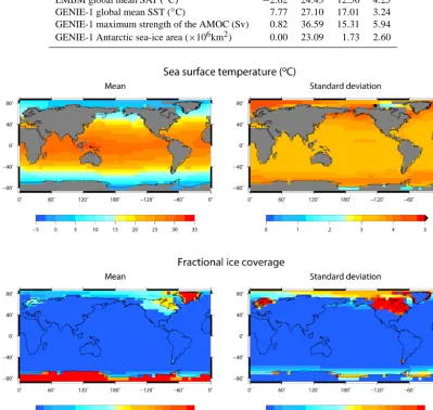
For each successful GENIE-1 simulation, surface output fields are extracted and used to force PLASIM for another 35 years. Each sampling plan, therefore, produces two equiv-alent ensembles of EMBM and PLASIM outputs. The fields used to initiate PLASIM simulations are SST, SIC and SIH as mentioned in Sect. 2. The 600-member ensemble mean and standard deviation of GOLDSTEIN SST and ice area are shown in Fig. 1. The ice coverage plotted is a combination of the fractional sea-ice cover from GOLDSTEIN sea ice (SIC) and the glacier mask described by ICF. The change in eleva-tion corresponding to each glacier mask is applied for both GENIE-1 and PLASIM.
varia-Table 2.A summary of the simulated climate states from the 600-member ensembles of GENIE-1 with EMBM and PLASIM.
Min Max Mean SD
PLASIM global mean SAT (◦C) −6.05 23.33 11.25 4.63
EMBM global mean SAT (◦C) −2.62 24.43 12.56 4.25
GENIE-1 global mean SST (◦C) 7.77 27.10 17.01 3.24
GENIE-1 maximum strength of the AMOC (Sv) 0.82 36.59 15.31 5.94 GENIE-1 Antarctic sea-ice area (×106km2) 0.00 23.09 1.73 2.60
Figure 1.The mean and standard deviation of SST and fractional ice coverage across the 600-member ensemble. The SST and sea-ice
coverage are prognostic output of GENIE-1 while the land ice coverage is regridded from Peltier ICE-5G. These fields, among others, are applied as surface boundary conditions to drive PLASIM atmosphere.
tions of the variable of interest within the specified parame-ter space. If this variable behaves non-linearly and exhibits a bifurcation, more simulations would be required to cap-ture such behaviour accurately. Second, the required number of simulations of cheap and expensive models are unknown. Different combinations of subsets with varying sizes are used and compared in the following section. It is ideal to generate a new design separately for each case but this is highly ineffi-cient and will result in an large incoherent ensemble with low reusability. Therefore, it is preferable to start with a large de-sign from which different subsets can be chosen. These sub-sets are all subjected to the same maximin criteria mentioned above. The algorithm used is covered in Sect. 4.2. While this
ensemble will be more reusable, a subset from it will most likely have a worse space-filling property than an indepen-dent MLH design of the same size. This is minimised by starting from a very large ensemble like the one employed here.
4 Statistical emulation
4.1 Gaussian process emulator
generally much cheaper to evaluate and, once validated, can be used in place of the full model to predict the observa-tion at untried choices of inputs. Our interest focuses on the Gaussian process (GP) emulator, also known as krig-ing (Rasmussen and Williams, 2006; Forrester et al., 2007), and a multi-level extension to this method, referred to as co-kriging (Kennedy and O’Hagan, 2000; Forrester et al., 2007; Cumming and Goldstein, 2008). The advantage of using the GP emulator is that the curve fits through the known points (training points from model runs at predefined sets of pa-rameters) and an estimated uncertainty is obtained for each emulated point.
To emulate a single summary quantity of the simulation outputs, for example, the global mean SAT, the assumptions made are as follows:
– The model output is a smooth function of its inputs.
– The model can be represented as a GP.
– Each emulator is concerned with a single deterministic scalar output.
The climate model,f(·), is a function of a set of param-eters, x=(x1,· · ·, xk), wherek is the number of perturbed
model parameters, which is 13 in this case. This number is commonly referred to as the number of dimensions of the emulator. The function f(·) is distributed as a GP with a mean function m(·) and a covariance function V(·,·). The mean function is given by
m(x)=hT(x)β, (1)
where h(x) is a vector of known regression functions. In the case of traditional kriging,hT(x)=1, makingβthe un-known overall mean. A variation of kriging, called universal kriging, uses a linear mean function:
hT(x)=(1,x), (2)
wherehT(x) is a (q×1) vector withq=k+1. Then
m(x)=β1+β2x1+ · · · +βk+1xk. (3)
The coefficients[β2, βk+1]now describe the expected trend of the simulator in response to each input.
The covariance function is given by
V(x,x0)=σ29(x,x0), (4)
whereσ2is the variance of the GP and9(., .) is the assumed correlation function:
9(x,x0)=exp "
−
k X
j=1 10θj
xj−x
0
j pj
#
. (5)
The function 9 describes the correlation between pairs of points, which is assumed to be stationary and continuous,
that is, it only depends on the distance between the pair of inputs, (x−x0). This exponential power form of covariance
structure is a popular choice due to its flexibility. Its assump-tion of staassump-tionarity might fail, for example, when there is a bifurcation in the system.
The value of9 depends on the correlation parametersp andθ, referred to as hyperparameters. θ is the correlation length parameter, defining how quickly the correlation be-tween the simulator outputs at two input points declines as the distance between them increases.θ indicates the activ-ity of the function in the corresponding dimension.p is a “smoothness” parameter of the correlation function. For sim-plicity and to reduce computational cost,pis assumed to be the same for all dimensions.
The specified GP is used as a prior for Bayesian infer-ence and is parameterised in terms of the hyperparameters β, σ2, θ and p. By analytically marginalising β and σ2, the marginal likelihood of the observed outputs atntraining points,y= [y1=f(x1),· · ·, yn=f(xn)], givenθandpcan
then be computed. A more detailed description of the deriva-tions and formuladeriva-tions can be found in Mardia and Marshall (1984). The estimatedθj in kriging and βj+1 in universal kriging indicate the relative activity in thejth corresponding dimension. Very low values of these hyperparameters imply inactive inputs. The dummy parameter, FFX, is included to verify that the emulator is doing a good job at identifying inactive inputs.
Prior beliefs about the model behaviour are combined with observations from training points to produce a posterior dis-tribution for the model. Having obtained estimates forθ and p, the posterior distribution found can be used to make pre-dictions about the model’s outputs at unsampled inputs. Full description of the derivation of the posterior distribution as well as distributional assumptions made forf(·),β andσ2 are available in Kennedy and O’Hagan (2001).
The exponential power form of covariance structure used here is a common choice due to its flexibility. Its assumption on stationary might fail, for example, when there is a bifur-cation in the system. The covariance specified, however, pro-vides a weak prior and as more training points are used, it contributes less to the final emulator.
4.2 Multi-level emulator
Co-kriging is an extension to the previously described tech-nique, which is applicable when a fast approximation of the primary simulator is available. In order for this method to work, the primary simulator and its approximation need to fulfil an additional assumption:
– The different levels of code are correlated and contain information about one another.
model can be built at a lower cost (Forrester et al., 2007). Potentially, this method can be extended to more code lev-els (Kennedy and O’Hagan, 2000), including the conceptual “reified” model (Goldstein and Rougier, 2009).
We make a simplification that the expensive and cheap models, fe andfc, respectively, can be represented by GP emulators of the same smoothness p. The cheap model is first emulated and then linked to the expensive one using the single multiplier approach:
fe(x)=ρfc(x)+fd(x). (6) The expensive function is modelled as the cheap GP multi-plied by a scaling factorρ, plus a separate GP,fd, modelling the stochastic residual of the expensive model (Kennedy and O’Hagan, 2000; Forrester et al., 2007). This approximation is chosen for its simplicity as well as the assumption that the main difference between the two models is a matter of scale, rather than changes in the shape or the location of the output. This assumption is made based on the fact that both models share the same ocean component and have the same inputs.
Two sets of training points are required for the construc-tion of a co-kriging emulator, a cheap setyc=fc(xc), which finely samples the input space, and a small sparse setye= fe(xe) of expensive points. Let the number of cheap and ex-pensive points bencandne, respectively.
When the number of PLASIM training points is small, such that a kriging emulator cannot be built with high ac-curacy, co-kriging employing an additional large number of training points from GENIE-1’s EMBM can be used instead. The number of points required depends on the size of the problem as well as the smoothness of the function being em-ulated. The inputs at which the expensive training set is ob-tained,xe, form a subset of the cheap set,xc. These expen-sive points are chosen using an exchange algorithm described by Cook and Nachtsheim (1980). A random subsetxeis se-lected and the Morris–Mitchell criterion is calculated. The first point x(1)e is then exchanged with each of the remain-ing points inxc. The exchange that gives the best Morris– Mitchell criterion is chosen. By repeating the same proce-dure for the remaining pointsx(2)e ,· · ·,x(ene), the “best” subset is obtained.
The covariance matrix for co-kriging,9ck, can be written in block form as
9ck=
σc2Ac(xc) ρσc2Ac(xc, xe) ρσc2Ac(xe, xc) ρσc2Ac(xe)+σe2Ae(xe)
, (7)
with Ac=9(x,x0;θc) andAe=9(x,x0;θe). This covari-ance matrix encompasses the correlation between cheap points (Ac(xc)), expensive points (Ac(xe) andAe(xe)) and the cross-correlation between the cheap and expensive points (Ac(xc, xe)). Details on the formulation and derivation of this equation can be found in Kennedy and O’Hagan (2000) and Forrester et al. (2007).
Both kriging and co-kriging emulators are constructed us-ing readily available software from Forrester et al. (2008).
4.3 Dimensional reduction using principal component analysis
So far, we have only discussed the use of GP emulators for single outputs. This can be a summary quantity such as the strength of the AMOC or the global average SAT (Hankin, 2005). The relevant output is, however, usually a high-dimensional array, containing fields and/or time series of many climate variables (e.g. SST, SAT or precipitation).
Climate variables at different spatial or temporal loca-tions can be emulated independently (Lee et al., 2012). This method, however, requires large computational power and ignores the covariances between outputs close to one another (Rougier, 2007). Other extension techniques using approaches that can capture the correlations between the outputs have been developed (Rougier, 2008; Conti and O’Hagan, 2010). However, these methods are not well suited for high-dimensional output.
In this work, we use principal component analysis (PCA) via singular value decomposition (SVD) to transform the high-dimensional data into a meaningful representation with lower dimensionality. While there are several techniques to accomplish this task, PCA is efficient and has the advan-tage that the leading components explain the majority of the variance across the ensemble (Holden and Edwards, 2010; Wilkinson, 2010). It is by far the most popular unsuper-vised linear technique. The mapping from the input parame-ter space to the reduced dimensional output space, specified by PCA, is the function being emulated instead of the direct input–output relationship. This method has been applied suc-cessfully in emulating temporally evolving spatial patterns of climate variables in Challenor et al. (2010), Holden et al. (2013) and Holden et al. (2014).
For each ensemble member, our field of interest, SAT, with dimension 64×32 is reshaped as a (2048×1) vector. The whole ensemble consisting ofnfields is represented by the (2048×n) matrix Y. Singular value decomposition is then performed on the centred matrix; i.e. the ensemble-averaged vector,µ, is removed:
Y−µ=LSRT, (8)
where L is the (2048×n) matrix of left singular vectors, also known as the empirical orthogonal functions (EOFs), S is the (n×n) diagonal matrix of singular values and r is the (n×n) matrix of right singular vectors, or the component scores. The product P of the singular values and the compo-nent scores is commonly known as the matrix of principal components (PCs):
P=S×RT. (9)
stationary spatial structures that constitute directions of vari-ability with no particular amplitude. The corresponding PC for each of these modes is the (n×1) column of P. Thenth element of each PC corresponds to thenth simulation from the training ensemble. These PCs provide the sign and the overall amplitude of the EOF corresponding to each simula-tion. They can, therefore, be considered as scalar functions of the input parameters and can be emulated using kriging or co-kriging. The number of training points,n, becomencand nefor the cheap and expensive emulator, respectively.
The EOFs and PCs of EMBM and PLASIM SAT can be obtained by decomposing each set separately. However, we are interested in using EMBM’s PCs as the cheap approxima-tion of PLASIM’s values; therefore, the SAT fields from both models are projected onto the same orthogonal basis vectors defined by PLASIM’s EOFs. This gives a new set of PCs for EMBM’s SAT:
Pr=LTe ×Yc. (10)
In other words, EMBM data (Yc) are rotated onto PLASIM’s coordinate system (Le) and the PCs obtained (Pr) are the ordinates of EMBM’s SAT fields in this new system. For co-kriging, the normal PCs are used as expensive training data from PLASIM while the rotated PCs are used as cheap train-ing data from EMBM.
The top (or high order) EOFs explain most of the variance in the data such that the dimension of Y can be reduced by keeping only the first q components (q < n). The elements of the PC vectors are now used as training data instead of the direct climate variable. We assume that these PCs also fulfil the same assumptions made for the climate variables. Emula-tors are built for the firstq PCs, providing an estimation,Pˆ, for an unknown input vector, i.e. the (214×13) input vector of the validation set. They are then used to work out the final prediction of the emulated field:
ˆ
Yil=µ+ q X
j=1
LijPˆTj l, (11)
whereYˆilis a component of the (2048×214) matrixYˆ.
The prediction, Yˆ, is different from the simulated value of Y by an error component, which can be decomposed into truncation error and component error. Truncation error is due to dimensional reduction. This is kept low by making sure that enough EOFs are retained to explain most of the vari-ance in the ensemble. Although there is no definite rule on what percent explained would be sufficient, a high value such as 90 % should be satisfactory. EOFs that explain less than 1 % of the total variance are often truncated since the data contained in them are often indistinguishable from random noise. Here, the first 10 EOFs are emulated and added pro-gressively. Validation is performed after each step and only EOFs, which contribute positively to the total variance ex-plained, are kept. Component error is a result of imperfect
estimation by the emulator, i.e. an error in estimating the cor-rect hyperparameters. This can be minimised by making sure enough training data are used to ensure the emulator can cap-ture the real trend of the ensemble. The GP emulator also provides an estimate of this error.
5 Results
5.1 Simulated climates
The EMBM output SATs are averaged over the final year of the 5000-year simulations while PLASIM output fields are averaged over the last 30 years. The ranges of some out-put variables obtained from the 600-member ensembles of GENIE-1 and PLASIM simulations are summarised in Ta-ble 2. The diversity of the output climate states is demon-strated by the large variation in SST, SAT, Antarctic sea-ice area and strength of the AMOC, which is weakened or shut down in some simulations. Because of the large upper limit of atmospheric CO2 concentration and GENIE-1’s general bias towards low Antarctic sea ice, in some simulations, the Southern Ocean appears to be completely ice free. The SAT in PLASIM is lower in general and exhibits a slightly larger variation compared to EMBM’s value.
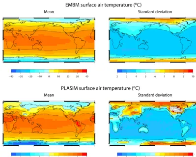
Figure 2 shows the ensemble mean and standard deviation of PLASIM and EMBM SAT. Although similar spatial pat-terns are seen in both, PLASIM exhibits a larger variation spatially and across the ensemble, especially at high eleva-tion. The comparison between the two models also shows that EMBM climate is much more zonal, with little land– sea difference. This is one of the known weaknesses of the energy–moisture balance model of the atmosphere, which is too diffusive (Lenton et al., 2006). A clearer distinction be-tween the ocean and the continents is modelled in PLASIM as shown in the standard deviation plot of Fig. 2.
Figure 2.The mean and standard deviation of SAT across the 600-member ensembles of GENIE-1 and PLASIM. There are white cells on the PLASIM SD plot where the outputs go beyond the plotted range. The largest standard deviation in PLASIM is 17.5◦C. The contours on the mean and SD plots are shown every 10 and 4◦C, respectively.
Interactions between the atmosphere and the ice sheets can also lead to larger variations due to orography or precipita-tion feedbacks. Their climate sensitivities will be explored later on with the help of the GP emulators constructed.
The resulting SAT from both models are compared against climatology in Fig. 3 using Taylor diagrams. These plots demonstrate the range of output obtained with respect to modern climate. The modern climate states here serve as reference points to better demonstrate the spread of the simulated ensembles as well as their differences. Both the standard deviations (SD) and root mean square differences (RMSD) are normalised (and non-dimensionalised) by divid-ing them by the SD of the observations. GOLDSTEIN SST from all simulation runs are compared with annual mean SST (1900–2005) from NOAA World Ocean Atlas (Locarnini et al., 2006). The SATs from the single-layer atmosphere EMBM are compared with annual mean surface air tem-perature over the period from 1979 to 2013 at the 1000 mb pressure surface from NCEP-DOE reanalysis-2 (Kanamitsu et al., 2002). The SATs from PLASIM are compared with the air temperature at 2 m from the same reanalysis. The sim-ulation runs with ice sheet configuration and CO2 concen-tration similar to those within the 1979–2013 period, ICF∈
{0,1,2,3,4}and 340 ppm<RFC<400 ppm, are highlighted in red. A plot showing the difference between the mean sur-face temperatures over this group of simulations and clima-tology is included in the Supplement (Fig. S1 in the Supple-ment).
The simulated pattern of SST correlates well with obser-vation (average correlation coefficient of 0.95), while the majority of the ensemble exhibits smaller spatial variabil-ity than climatology (average normalised SD of 0.85). The spread in these modern GOLDSTEIN SST points is due to the large range of the varied GENIE-1 parameters. The stan-dard deviations of SAT are also underestimated in EMBM (average normalised SD of 0.83). PLASIM SAT correlate well with the climatology (average correlation coefficient of 0.97). The spatial variation in PLASIM SAT has a similar mean to EMBM but has a larger range (both ensembles have average normalised SD of 0.83).
5.2 Scalar emulation
Reanalysis Simulation
Simulation with modern ICF and RFC
Figure 3.Taylor diagrams showing a comparison between model runs with climatology: GOLDSTEIN SST (left), EMBM SAT (middle)
and PLASIM SAT (right). The magenta dots represent reanalysis taken from Locarnini climatology (1900–2005) (Locarnini et al., 2006) (left), NCEP-DOE reanalysis 2 annual mean SAT (1979–2013) at 1000 mb (Kanamitsu et al., 2002) (middle) and NCEP-DOE reanalysis 2 annual mean SAT (1979–2013) at 2 m (Kanamitsu et al., 2002) (right). The points highlighted in red represent runs with ICF∈ {0,1,2,3,4} and 340ppm<RFC<400 ppm.
ror (RMSE) between the simulated and emulated validation points (Sect. 3.2) are computed and then used as indications of the validity of the emulator. The coefficient of determina-tion,r2, is the square of the sample correlation coefficient:
r2= cov(Y,bY) p
var(Y)var(bY))) !2
. (12)
More training points are gradually added to produce more ac-curate emulators with decreasing RMSE and increasing r2. At approximately 200 points (nc=200), adding more train-ing data no longer significantly reduces the RMSE value. It is concluded that approximately 200 cheap points are suffi-cient to capture the variation over the EMBM output space. We then attempt to build co-kriging emulators for global mean SAT in PLASIM using 200 cheap points and additional expensive data points. Again, 30 expensive points are cho-sen for initial training. It is found that 50 PLASIM points (ne=50) are enough to construct a good emulator with RMSE=0.51◦C andr2=0.98.
The number of training points required varies from one emulator to another since it depends strongly on the func-tion being emulated. As the number of parameters increases, the dimension of the emulator also increases and hence more training points are required. Typically an average of 10 points per dimension is assumed. This, however, depends on how linear or how “active” the function is. A highly non-linear function might require many more points while a more linear function might not need as many as 10 points per di-mension.
Kriging emulators using only expensive points are also constructed to provide comparison between the two tech-niques. When the same amount of training data is used, co-kriging outperforms co-kriging. More expensive points are then
added to improve the kriging emulator until a similar value of RMSE is obtained. In this case, the kriging emulator using ne=200 PLASIM training points gives RMSE =0.50◦C andr2=0.98. Therefore, co-kriging achieves of the same level of accuracy with only 25 % as much expensive data.
A second pair of emulators is produced for the global SAT anomaly from SST (global annual mean SAT minus SST). In this case, the component of the SAT response that is a trivial function of the boundary conditions is removed. Fol-lowing the procedure described above, a co-kriging emula-tor using 70 expensive points and 250 cheap points were constructed and compared to a kriging emulator using only 70 expensive points. The RMSE andr2are included in Ta-ble 4. The co-kriging emulator obtains RMSE=0.31◦C and r2=0.95. This time, a kriging emulator using 100 expensive points gives similar validation result, RMSE=0.33◦C and r2=0.92. The co-kriging emulator still manages to utilise meaningful information from EMBM, albeit not as well as in the previous example, and reduces the expensive points needed by approximately 30 %.
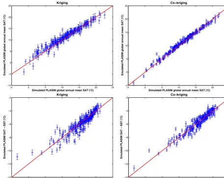
For both kriging and co-kriging emulators using the same expensive training points, the emulated global mean SATs at the 214 validation points are plotted against their simulated values (Fig. 4). The corresponding RMSE andr2values are shown in Table 3. Tables 3, 4 and Fig. 4 show that the co-kriging emulators reproduce the simulated values more accu-rately. Tables 3 and 4 also contains the ensemble mean and standard deviation from both co-kriging and kriging emula-tors, compared with the true values obtained from the simu-lated ensemble.
be-Table 3.Validation results for kriging and co-kriging emulators of PLASIM global mean SAT. The co-kriging emulator uses 50 expensive points and 200 cheap points while the kriging emulator here uses the same 50 expensive points.
Kriging emulator Co-kriging emulator Simulated ensemble
RMSE (◦C) 0.93 0.51 N/A
r2 0.94 0.98 N/A
Ensemble mean (◦C) 10.96 11.30 11.40
Ensemble SD (◦C) 4.89 4.73 4.57
Table 4.Validation results for kriging and co-kriging emulators of PLASIM global mean SAT – SST. The co-kriging emulator uses 70
expensive points and 250 cheap points while the kriging emulator here uses the same 70 expensive points.
Kriging emulator Co-kriging emulator Simulated ensemble
RMSE (◦C) 0.42 0.31 N/A
r2 0.91 0.95 N/A
Ensemble mean (◦C) −5.81 −5.77 −5.72
Ensemble SD (◦C) 1.65 1.70 1.50
tween simulated and emulated values from the co-kriging emulators are over 0.90 for both. The standard deviations across the ensembles are slightly overestimated in both em-ulators. From the figure, the emulated values can be seen to deviate more for larger anomalies.
The uncertainty in the emulator predictions, arising from not having evaluated the model at untried input configura-tions, is called the “code uncertainty” (O’Hagan, 2006). An advantage of the GP emulator employed is that we can quan-tify this uncertainty, which is represented as the error bar at each prediction in Fig. 4. The additional information from the cheap training data helps reduce this uncertainty for the co-kriging emulator.
5.3 EOF decomposition
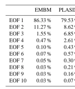
The following analysis attempts to explain the processes and parameters that determine the spatial distributions of SAT in GENIE-1 and PLASIM using PCA. SVD was applied to two (2048×n) matrices of EMBM and PLASIM SAT fields, wheren=nc=ne=660. Over 99 % of the variance across the ensemble in these fields can be explained by the top 10 EOFs, as shown in Table 5. This indicates that they are sufficient to generate a good approximation to the simulated responses. As suggested from the emulator for global mean SAT, less than 600 points would be sufficient for the emu-lators. To ensure that the decomposition is robust, SVD is applied on smaller subsets (n=30 ton=250). The EOFs appear to be qualitatively the same. Only minor quantita-tive differences are obtained, therefore, the EOFs and PCs are judged as robust and representative of the ensemble be-haviour. These subsets are chosen using the same exchange algorithm mentioned in Sect. 4.2 to obtain designs that give the best space-filling Morris–Mitchell criterion (Morris and Mitchell, 1995).
Table 5. Percentage of variance in SAT, explained by the first
10 EOFs for GENIE-1 with EMBM and with PLASIM. The 150-member ensembles are used to obtain these values.
EMBM PLASIM
EOF 1 86.33 % 79.53 %
EOF 2 11.27 % 8.62 %
EOF 3 1.55 % 6.85 %
EOF 4 0.47 % 2.61 %
EOF 5 0.10 % 0.43 %
EOF 6 0.07 % 0.57 %
EOF 7 0.05 % 0.30 %
EOF 8 0.03 % 0.21 %
EOF 9 0.03 % 0.16 %
EOF 10 0.03 % 0.07 %
Total 99.93 % 99.35 %
The high percentage of variance explained by the retained EOFs mean that by successfully emulating them, the SAT field of PLASIM can be accurately estimated. For EMBM data to be useful, its EOFs and PCs need to carry meaning-ful information about PLASIM’s modes. To verify this, an analysis of the EOFs and PCs of the two models are carried out.
parame-−5 0 5 10 15 20 25 −10
−5 0 5 10 15 20 25
Simulated PLASIM global annual mean SAT (°C)
Emulated PLASIM global annual mean SAT (
°
C)
Kriging
−5 0 5 10 15 20 25
−5 0 5 10 15 20 25
Simulated PLASIM global annual mean SAT (°C)
Emulated PLASIM global annual mean SAT (
°
C)
Co−kriging
−14 −12 −10 −8 −6 −4 −2
−14 −12 −10 −8 −6 −4 −2
Simulated PLASIM SAT − SST (°C)
Emulated PLASIM SAT − SST (
°
C)
Kriging
−14 −12 −10 −8 −6 −4 −2
−14 −12 −10 −8 −6 −4 −2
Emulated PLASIM SAT − SST (
°
C)
Simulated PLASIM SAT − SST (°C)
Co−kriging
Figure 4.The upper panels show PLASIM simulated global mean SAT at the 214 validation points plotted against their emulated values from both kriging (left) and co-kriging (right) emulators. The error bars indicate a 2 standard deviation interval at each point. The lower panels show the results of the global mean SAT–SST emulators.
ters were varied. Also, the mean function is linear so they do not contain information on the non-linearity of the emu-lated function. They also inherit uncertainties from imperfect emulation.
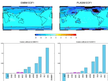
The first EOF for both models is of the same sign globally, suggesting a change in the radiation budget due to the green-house gas and the albedo effects. The effects due to chang-ing glacier condition and atmospheric CO2concentration are accentuated in PLASIM because corresponding changes are taken into account in PLASIM. According to the emulator coefficients, the largest contributions are due to RFC, OL0, RMX and ICF in both PLASIM and EMBM. Large values of ICF result in a lower global mean SAT due to higher albedo. Large values of RFC, OL0 and RMX, on the other hand, have the opposite effect on global mean temperature due to more heat being absorbed by the increased greenhouse gas content in the atmosphere. Hence, ICF has the opposite sign to RFC, OL0 and RMX.
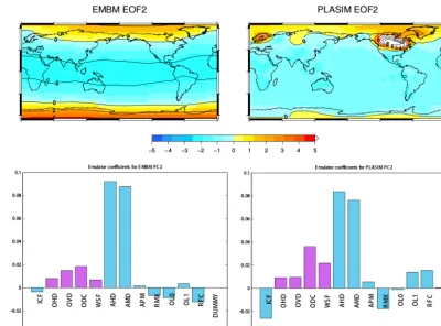
The second EOFs in EMBM and PLASIM exhibit changes of opposite sign at Equator and polar regions, reflecting a re-distribution of the heat budget (Fig. 6). The parameters con-trolling heat diffusivity in the atmosphere (AHD and AMD) play the largest role in this process. While they dominate the signals, there are smaller contributions from the ocean heat diffusivity parameters (OHD and OVD), which have similar but smaller effects compared to AHD and AMD. Other small signals do not necessarily agree with each other; i.e., RFC has opposite signs in the two models.
With emulator coefficients of approximately 0, the dummy variable is correctly identified as an inactive parameter in all cases (Figs. 5 and 6), giving us more confidence in using the coefficients. Any parameter with coefficients of comparable magnitude to FFX is also assumed to be inactive, such as OHD and OVD for EMBM and PLASIM’s first EOF.
co-Figure 5.The first EOFs of EMBM and PLASIM SAT (upper) and the universal kriging emulator coefficients of their corresponding PCs (lower). All 600 data points are used to train each of these emulators. The black cells in PLASIM EOF1 indicate values lower than the plotted range. Contours are drawn over both plots at a 2◦C interval.
kriging. The extra training points from EMBM, therefore, are expected to provide inference on PLASIM’s behaviour. Each pair of PCs from EMBM and PLASIM form a set of cheap and expensive training data for the corresponding emulator. Even though this is applied to all 10 PCs, according to Ta-ble 5, only the first 4 modes contribute significantly to the total variance. Lower-order modes appear indistinguishable to noise. It is difficult to emulate them independently and so it is unlikely that any meaningful relationship between them can be found by co-kriging.
Although all 600 data points are used to train each of these emulators, results obtained from smaller subsets show no systematic differences.
The assumptions made for Eq. (6) are expected to hold in the case of emulating PLASIM’s PCs. The emulator coeffi-cients in Figs. 5 and 6 show that the PCs of the two models exhibit similar trends due to the varying input parameters. The difference in the magnitude of the contributions from these parameters should be sufficiently approximated using a scaling constant,ρ, and a stochastic process,fd. The spatial pattern in PLASIM, however, depends on the EOFs and so different regional responses compared to EMBM can still be emulated using this method.
5.4 Emulation of 2-D output fields
We retained the first 10 EOFs of EMBM and PLASIM SAT, which describe 99.93 and 99.35 % of the simulated ensem-ble variance, respectively (Taensem-ble 5). Each individual field can be approximated as a linear combination of these 10 EOFs, scaled by their respective PCs according to Eq. (8). Using this method of dimensional reduction, only 10 emulators or less are needed instead of 2048 emulators if each individual grid point is emulated. Both kriging and co-kriging emula-tors are then constructed for each of these PCs.
Using the same procedure as described in Sect. 5.2, ex-ploratory exercises show that approximatelync=150 train-ing points are needed to obtain a good emulator of the EMBM SAT fields. The cheap data are, therefore, the 150 indices of each of the first 10 rotated PCs of the (2048×150) matrix of GENIE data. It is found that atne=50, we obtain a co-kriging emulator that validates well against simulated values.
Figure 6.The second EOFs of EMBM and PLASIM SAT (upper) and the universal kriging emulator coefficients of their corresponding PCs (lower). All 600 data points are used to train each of these emulators. The white cells in PLASIM EOF2 indicate values higher than the plotted range. Contours are drawn over both plots at a 2◦C interval.
co-kriging reduces the required expensive training data to one-third of the amount needed when using kriging.
The co-kriging (trained with 50 expensive and 150 cheap points) and kriging (trained with 50 expensive points) are val-idated using the 214-member validation set. Both the individ-ual PCs and the final reconstructed SAT are validated against true values. First, to test the emulator’s ability to reproduce PC values, each emulated PC is validated against those de-composed from the simulated ensemble (Table 6). For the first score, co-kriging emulator validated very well with an r2 value of 0.97. Lower-order PC coefficients are generally harder to emulate; hence, the value ofr2decreases down the list. It is possible that they reflect physical processes that are more difficult to represent as simple functions of the input pa-rameters or simply represent stochastic processes. With a low value ofr2, the emulator does little more than adding some random noise, e.g. from the 6th to the 10th PCs, with the ex-ception of the 9th. There are several reasons for this. First, the PCs of EMBM might reflect random noise and so can-not be emulated. Since the cheap emulators are can-not meaning-ful, the expensive ones can gain no useful information. Sec-ond, PLASIM’s PCs might be noise and co-kriging fails to work for the same reason. Finally, the relationships between EMBM and PLASIM PCs might not have been successfully
determined. This either means that EMBM did not contain the information on these PLASIM’s modes or the emulator fails to determine it. Even though the signal from the 9th mode is very small, it was emulated with some success. De-spite the fact that mode 6, 7, 8 and 10 were not emulated successfully, co-kriging still performs either comparably or better than kriging.
The 10 co-kriging emulators of PLASIM PCs are then used to reconstruct the SAT fields at each validation point. To validate the simulated SAT fields, the quality of the in-dividual emulations and the spatial pattern of the emulated field are tested. In order to test the proportion of the total ensemble variance captured by the emulator:
VT =1−
59 X
n=1 2048 X
i=1
(Sn,i−En,i)2
59
X
n=1 2048 X
i=1
(Sn,i− ¯Si)2, (13)
whereSn,i is the simulated output at grid celli in the nth
member of the validating ensemble,En,iis the corresponding
emulated output andS¯ithe ensemble mean simulated output
at grid celli.VT assesses the error in the emulator for each
Table 6.Validation of each PC emulator using the 59-member ensemble. The correlation coefficients show how well matched the emulated PCs are compared with the simulated values. The co-kriging emulator uses 50 expensive points and 150 cheap points while the kriging emulator here uses the same 50 expensive points.
Principal component emulator
1 2 3 4 5 6 7 8 9 10
Krigingr2 0.91 0.75 0.84 0.50 0.15 0.04 0.00 0.09 0.24 0.00
Co-krigingr2 0.97 0.83 0.84 0.64 0.18 0.05 0.02 0.10 0.24 0.00
the whole validation set.VT and RMSE are used in
combi-nation to assess the emulator validity.
Figure 7 demonstrates the effect of each added PC to the value of VT and RMSE. When only the first emulated
component is considered, the co-kriging emulator reproduces 76.2 % of the simulated variance (averaged over all space and all ensemble members), which is close to the 79.5 % vari-ance explained by the first EOF (Table 5). This is also re-flected by the high degree of accuracy of the PC 1 emulator (Table 6). The addition of the next four emulated compo-nents brings the percentage of simulated variance being cap-tured,VT, to 93.2 %, close to the total amount of 98.0 %
ex-plained by the first five EOFs (Table 5). The average RMSE is 1.33◦C, which is approximately 1.7 % of the average spa-tial variation in temperature or 4.8 % of the average varia-tion across the whole ensemble at each grid point. The last five emulated PCs have a negligible effect on both VT and
RMSE. Among these, only the 9th PC improves the overall result while the others worsen it. For the kriging emulators, the same behaviour is observed but with lower accuracies. The maximum variance explained by the kriging emulators is 85.3 %. Also included in Fig. 7 are lines corresponding to the validation results if the emulators were perfect. These demonstrate the errors introduced by the dimensional reduc-tion process.
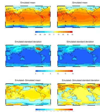
Figure 8 shows the emulated and simulated spatial pattern of the ensemble mean and standard deviation. The differ-ences between these emulated and the simulated fields are within 1◦C. Therefore, the ensemble behaviour is well re-produced. There is, however, a slight underestimation of the SD over the Northern America continent where the glacier mask is applied. The 2-D SAT emulator appears to underes-timate the ensemble variance by a small amount. The error seen is a combination of the two types of errors introduced in Sect. 4.1. Despite having very different outputs (Fig. 3), the method proposed successfully utilises GENIE-1’s EMBM output to aid the construction of PLASIM SAT emulator.
In the work presented here, only annually averaged fields are considered. The generalisation to emulate monthly aver-age fields or seasonal cycles is straight forward. We simply have to replace the current (2048×1) annual-averaged maps with a (24576×1) map of the 12 monthly averaged fields.
Figure 7. Comparison between kriging (dashed line) and
co-kriging (solid line) emulators. The variance explained (blue) when each PC is added is shown together with the RMSE (red) of the corresponding reconstructed validation SAT fields. The dot-dashed lines represents the same values obtained if the emulator were per-fect. The deviations of these line from RMSE=0◦C and V = 100 % are errors introduced by dimensional reduction.
5.5 Relationship with the coupled system
Figure 8.Mean and standard deviation of the emulated (upper and middle left) and simulated (upper and middle right) validating ensembles. The emulated–simulated differences in mean (lower left) and standard deviation (lower right) are also shown.
been employed to reproduce the output of AOGCMs under a large range of forcing scenarios (Holden et al., 2014; Cas-truccio et al., 2014). Our multi-level emulation technique of-fers an alternative method to reproduce the key character-istics of an AOGCM using only a small training set, given a larger ensemble of a cheaper model of the same system, covering unsampled CO2 concentrations. Another example where our technique can be applied is in emulating a carbon cycle model to provide an estimation of the atmospheric CO2 concentration as a function of a time series of anthropogenic CO2emissions and non-CO2radiative forcing (Foley et al., 2016). CO2concentration from coupled climate–carbon cy-cle models can be emulated and replace the simple carbon
cycle component often used in integrated assessment mod-els.
In reality, changes to the climate system components that are focused on will feed back on other climate system com-ponents; i.e., if the present study were extended to the fully coupled system, differences in SAT, wind stress and the hy-drological cycle between PLASIM and the EMBM would feed back on SST and sea-ice distribution.
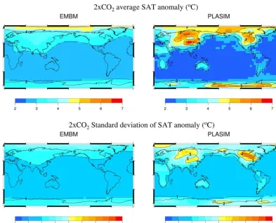
Figure 9.Mean (upper panel) and standard deviation (lower panel) of the SAT anomaly corresponding to a double in atmospheric CO2 concentration in EMBM and PLASIM.
the basis of two new designs. ICF is fixed at 0 for both sets. Climate sensitivity is defined as the warming response to a doubling of atmospheric CO2from the pre-industrial values. Hence, a control set (CTRL) has RFC set to 278 ppm and another set (2×CO2) has RFC set to 556 ppm. The emula-tors constructed in the previous section are used to predict the SAT fields resulting from these two designs. This process can be done within seconds, at almost no additional compu-tational cost.
The average SAT anomalies due to a doubling of at-mospheric CO2 concentration for both models, 2×CO2− CTRL, are shown in Fig. 9. The area-weighted global mean SAT are used to calculate the probability distribution of cli-mate sensitivity for the two models, shown in the upper panel of Fig. 10. The means of the two distributions are1TCO2of 2.99±0.91◦C for EMBM and 3.37±0.95◦C for PLASIM. Figure 10 shows that the climate sensitivities in the two mod-els have similar distributions with means differing by ap-proximately 0.38◦C. The range is broad due to the parame-ters varied. PLASIM displays larger changes in temperature over the continent in general and especially over high ele-vation areas (Fig. 9). Because of this, the average anomaly 1TCO2 in a PLASIM simulation is larger than the
corre-sponding value in EMBM. The relationship between the two distributions is approximately linear, as shown in the lower panel of Fig. 10. Since no PLASIM parameter is varied apart from ICF and RFC (which are both held constant in this ex-periment), PLASIM climate sensitivity is heavily influenced by the GOLDSTEIN surface conditions.
1 2 3 4 5 6 7 0
0.1 0.2 0.3 0.4 0.5 0.6
Global mean SAT anomaly (°C)
EMBM PLASIM
1 1.5 2 2.5 3 3.5 4 4.5 5 5.5 6
1 2 3 4 5 6 7
EMBM anomaly (°C)
PLASIM anomaly (
°
C) y=1.037x+0.266
Figure 10.The upper panel shows the probability distributions of EMBM (red) and PLASIM (blue) climate sensitivities. The mean of each distribution is denoted by the dot-dashed line of the same colour. The lower panel shows a plot of PLASIM anomalies against EMBM anomalies. The coefficients of the linear function fitted through the data are included in the figure.
with GOLDSTEIN ocean and sea-ice components. Atmo-spheric output from PLASIM, such as SAT, precipitation and wind stress can be emulated as a function of the pre-scribed SST and used, in return, as boundary conditions for the ocean. This framework would be able to capture some processes, which are currently not adequately modelled or not represented at all in EMBM. There are certain implica-tions for when such a framework would be useful since the emulators are built upon a collection of steady-state simula-tions where only one-way interaction between PLASIM and the ocean component is available. This type of framework would not be suitable in the context of processes such as ENSO (El Niño–Southern Oscillation) in which the atmo-sphere and ocean vary together on interannual timescales. However, it may be useful when events with much longer timescales, where the atmosphere can regarded as being at equilibrium with the ocean, are considered. While informa-tion on chaotic higher-frequency atmospheric variability is lost, extra information from the higher-fidelity atmospheric model is gained without incurring a large computational cost.
6 Summary and conclusions
We have described in this paper the development and evalu-ation of large ensembles of GENIE-1 and PLASIM simula-tions for application in statistical emulation.
For this work, we employ the non-parametric fitting method of Gaussian process emulation. Two variations of this well-established method, kriging and universal kriging, are briefly described in Sect. 4.1. Compared to polynomial
fitting techniques, such as the one employed by Holden et al. (2014), this approach provides an estimate of the uncertainty introduced by the emulation process, also referred to as “code uncertainty”.
To efficiently extend this method from emulating scalar output to emulating high-dimensional output, e.g. the 2-D SAT fields, principal component analysis is used. This pow-erful technique decomposes the output surface fields of both EMBM and PLASIM models into orthogonal EOFs, scaled by the respective PCs. The EOFs are, however, statistical modes and direct connection to physical processes cannot always be drawn directly. Emulator coefficients of the PCs corresponding to these modes, however, can provide a link between them and the varying model parameters, allowing for better interpretation of the model behaviour. It also allow us to identify and preserve the correlation between grid cells. Here, the first five PCA modes are emulated instead of in-dividual grid cell values, reducing the computational cost sig-nificantly. Although not explored in this work, the links be-tween different model outputs may also be exploited to allow for further reduction of dimension when emulating multivari-ate output.
A multi-level emulation technique, co-kriging, is used to build both scalar and high-dimensional output emulators for PLASIM with additional information from EMBM. The con-structed co-kriging emulators successfully estimate both the global mean SAT and the 2-D array of SAT fields of PLASIM as functions of the 13 GENIE-1 parameters. Being cheaper to evaluate, EMBM can be used to sample GENIE-1’s parame-ter space more finely, providing information where PLASIM data are sparse. Despite being structurally unrelated, the link between EMBM and PLASIM is successfully established, resulting in PLASIM emulators being built using a smaller amount of expensive data. The combination of PCA with co-kriging allows us to emulate accurately the spatial pattern of PLASIM SAT despite the model having a different response to EMBM’s. Emulated outputs are validated against simu-lated values using a separate validation ensemble. Both spa-tial pattern and magnitude of SAT are well reproduced across the ensemble. Apart from the ensemble mean and standard deviation, individual simulations are also successfully emu-lated with high accuracy. The emulators, however, show a tendency to underestimate the variance spatially and across the ensemble. This is unavoidable because of the dimensional reduction process. The quantification of the emulator uncer-tainties are beyond the scope of this paper and should be ex-plored in further studies in order to improve the emulators’ performance.
equiva-lent in EMBM. However, it is possible that other GENIE-1 fields might be more suitable as the fast approximation to PLASIM’s PPTN, e.g. SST or elevation. Work has been done in the past using elevation as a fast approximation for PPTN (Hevesi et al., 1992).
This work establishes the technique for emulating the equilibrium response of the model. Compared to available efficient frameworks such as the MIT IGSM-CAM (Mas-sachusetts Institute of Technology – Integrated Global Sys-tem Model linked with the National Center for Atmospheric Research (NCAR) Community Atmosphere Model) (Monier et al., 2013), a present limitation of this technique is in the scope for two-way coupling (e.g. in the present study the PLASIM atmosphere passively responds to the ocean). How-ever, a future study will show that it is possible to emulate the atmospheric fields (precipitation, surface winds, etc.) that di-rectly influence other model components and use these as boundary conditions. This technique has the limitation that the atmosphere is treated as being in a steady state with the ocean, so that the effect of interannual variability cannot be explicitly represented, but would nevertheless be of value for modelling long-timescale phenomena such as glacial-interglacial cycles.
We have demonstrated that multi-level emulation across structurally unrelated models provides useful information more efficiently than using either model in isolation. Sev-eral challenges remain before a coupled model making use of such an emulator can be constructed, and the steady-state vs. transient issue is one of them. The seasonality, which is currently lacking, will also be included by the modification described in Sect. 5.4. PLASIM’s parameters, which do not have an equivalent in EMBM, are not yet considered. The current experiment design does not allow for the effect of aerosols, sea ice or vegetation to be studied. It simply at-tempts to improve the current simulated climate in GENIE-1 by incorporating the dynamic of PLASIM atmosphere. The role of these parameters will likely be explored in future stud-ies.
The advantage of the emulation technique used here is that it does not depend on a fix set of models and can be applied to a wide range of models for different applications. It also pro-vides a useful tool in coupling models of different fidelity and resolutions. The emulators, however, are built for specific ap-plications and so care should be taken to avoid extrapolating beyond the emulated space.
In conclusion, the work presented here demonstrates a concept with applications in not only climate research but ex-tending to a wide range of problems where multi-level com-puter models are available.
The Supplement related to this article is available online at doi:10.5194/ascmo-2-17-2016-supplement.
Edited by: C. Forest
Reviewed by: four anonymous referees
References
Castruccio, S., McInerney, D. J., Stein, M. L., Crouch, F. L., Jacob, R. L., and Moyer, E. J.: Statistical emulation of climate model projections based on precomputed GCM runs, J. Climate, 27, 1829–1844, 2014.
Challenor, P. G., McNeall, D., and Gattiker, J.: Assessing the proba-bility of rare climate events, in: The Oxford handbook of applied bayesian analysis, edited by O’Hagan, A. and West, M., chap. 16, 403–430, Oxford University Press, New York, 2010.
Conti, S. and O’Hagan, A.: Bayesian emulation of complex multi-output and dynamic computer models, J. Stat. Plan. Infer., 140, 640–651, doi:10.1016/j.jspi.2009.08.006, 2010.
Cook, R. D. and Nachtsheim, C. J.: A comparison of algorithms for constructing exact D-optimal designs, Technometrics, 22, 315– 324, 1980.
Cumming, J. and Goldstein, M.: Small Sample Designs for Com-plex High-Dimensional Models Based on Fast Approximations, Technometrics, 51, 377–388, 2008.
Edwards, N. R. and Marsh, R.: Uncertainties due to transport-parameter sensitivity in an efficient 3-D ocean-climate model, Clim. Dynam., 24, 415–433, doi:10.1007/s00382-004-0508-8, 2005.
Edwards, N. R., Cameron, D., and Rougier, J.: Precalibrating an in-termediate complexity climate model, Clim. Dynam., 37, 1469– 1482, doi:10.1007/s00382-010-0921-0, 2011.
Foley, A. M., Holden, P. B., Edwards, N. R., Mercure, J.-F., Salas, P., Pollitt, H., and Chewpreecha, U.: Climate model emulation in an integrated assessment framework: a case study for mitigation policies in the electricity sector, Earth Syst. Dynam., 7, 119–132, doi:10.5194/esd-7-119-2016, 2016.
Forrester, A., Sobester, A., and Kean, A.: Engineering design via surrogate modelling, vol. 1, John Wiley & Sons, Ltd, Chichester, 2008.
Forrester, A. I., Sóbester, A., and Keane, A. J.: Multi-fidelity opti-mization via surrogate modelling, P. R. Soc. A, 463, 3251–3269, doi:10.1098/rspa.2007.1900, 2007.
Fraedrich, K., Jansen, H., Kirk, E., Luksch, U., and Lunkeit, F.: The Planet Simulator: Towards a user friendly model, Meteorologische Zeitschrift, 14, 299–304, doi:10.1127/0941-2948/2005/0043, 2005.
Goldstein, M. and Rougier, J.: Reified Bayesian modelling and in-ference for physical systems, J. Stat. Plan. Infer., 139, 1221– 1239, doi:10.1016/j.jspi.2008.07.019, 2009.
Haberkorn, K., Sielmann, F., Lunkeit, F., Kirk, E., Schneidereit, A., and Fraedrich, K.: Planet Simulator Climate, Tech. rep., Meteo-rologisches Institut, Universität Hamburg, 2009.