R E S E A R C H
Open Access
On the influence of interpolation method
on rotation invariance in texture recognition
Gustaf Kylberg
1and Ida-Maria Sintorn
1,2*Abstract
In this paper, rotation invariance and the influence of rotation interpolation methods on texture recognition using several local binary patterns (LBP) variants are investigated.
We show that the choice of interpolation method when rotating textures greatly influences the recognition capability. Lanczos 3 and B-spline interpolation are comparable to rotating the textures prior to image acquisition, whereas the recognition capability is significantly and increasingly lower for the frequently used third order cubic, linear and nearest neighbour interpolation. We also show that including generated rotations of the texture samples in the training data improves the classification accuracies. For many of the descriptors, this strategy compensates for the shortcomings of the poorer interpolation methods to such a degree that the choice of interpolation method only has a minor impact. To enable an appropriate and fair comparison, a new texture dataset is introduced which contains hardware and interpolated rotations of 25 texture classes. Two new LBP variants are also presented, combining the advantages of local ternary patterns and Fourier features for rotation invariance.
Keywords: Local binary patterns, Texture dataset, Filter banks
1 Introduction
In many computer vision and image analysis applications, the texture of an object is an important property that can be utilized for classification or segmentation procedures. However, texture analysis in digital images is not a trivial task and numerous texture descriptors have been pro-posed. In some applications, e.g. face recognition as in [1], the orientation of the object is known, while in many other applications the orientation of an object may be arbitrary and hence also the texture. In the latter case, the texture can be rotated to a main orientation or principal direction, see e.g. [2] where the Radon transform is used to accom-plish this, or alternatively, a texture descriptor invariant to rotation can be used. A third way to achieve rotation invariance is to add rotated versions of the textures to the training data. This technique of adding a priori infor-mation to achieve invariance towards something through adding virtual training samples is explored in [3].
*Correspondence: [email protected]
1Vironova AB, Gävlegatan 22, SE-11330 Stockholm, Sweden 2Uppsala University, Department of Information Technology, Lägerhyddsvägen 20, SE-75105 Uppsala, Sweden
Rotation invariant texture descriptors have been widely studied, as reviewed in [4]. Texture descriptors invari-ant to viewpoint (adding even more degrees of freedom) have also been studied in for example [5]. However, the problem of arbitrary viewpoints is not addressed in this paper.
Rotation invariance for a texture descriptor can be achieved locally (at each pixel position) or globally (for the region/patch investigated). In [6], clusters of filter bank responses, denoted textons, are computed and the his-togram of occurring textons are used as features. They propose a filter bank, denoted MR8, for which global rotation invariance is achieved by using the maximum response over six different orientations. A possible advan-tage with globally rotation invariant descriptors is that such a descriptor can retain the distribution of local ori-entations while this information will be lost in a local rotational invariant descriptor. Note however, that in the case of MR8, this information is lost when only keeping the maximum response over orientations. In [7], a glob-ally rotation invariant descriptor retaining distributions over orientations is introduced based on Fourier trans-formed responses from Gabor filter banks. In [8], a local rotation invariant descriptor is introduced based on the
local binary pattern (LBP) descriptor and [9, 10] proposed globally rotation invariant descriptors based on Fourier transformed of the LBP.
The LBP descriptor has over the past decades resulted in a whole family of texture descriptors. For this study on rotation invariance, we have selected the classic LBP descriptor together with seven extensions, including two different approaches to rotation invariance. The descrip-tors are the following: (i) the classicLBPdescriptor [8], (ii)
LBPri—the approach to local rotation invariance [8], (iii)
LBPDFT—an approach to rotation invariance where glob-ally rotation invariant Fourier features are extracted [10], (iv) ILBP(improved LBP) which is a more noise robust extension of the LBP [11], (v)ILBPriusing the approach to local rotation invariance, (vi)ILBPDFTusing the approach to global rotation invariance, (vii)LTPDFT(local ternary patterns) where three rather than two states are con-sidered in the local neighbourhood ([12]) and using the approach to global rotation invariance, (viii) ILTPDFT combining ILBP, LTP and the approach to global rotation invariance. By studying these descriptors, we can get a baseline performance from the classic LBP and see how two well used extensions to the LBP perform. In addition, we can see how invariant the two different approaches to rotation invariance are.
In this paper, we investigate and compare the follow-ing: local rotation invariance, global rotation invariance, including rotations in the training data, and the effect of the different interpolation methods when rotating tex-tures, in the setting of retaining discriminant texture information. In order to do this, we introduce a new tex-ture dataset, the Kylberg Sintorn Rotation Dataset. The dataset includes images of hardware-rotated textures as well as texture images rotated by the interpolation ker-nels: nearest neighbour, linear, third order cubic, cubic B-spline and Lanczos 3. The dataset has 25 classes of dif-ferent types of textured surfaces and is publicly available [13]. The images in the dataset are acquired in raw format avoiding compression artefacts.
2 The Kylberg Sintorn rotation dataset
There are, to our knowledge, two texture datasets avail-able which contain images of rotated textures; the Outex dataset [14] and the Mondial Marmi dataset [10].
The Mondial Marmi dataset contains images of slabs of Italian marble. The textured surfaces are rotated prior to image acquisition to allow for studying rotation invariance in texture analysis. The imaging is done with a compact camera storing the images in JPEG format with notable compression artefacts.
The Outex dataset is a large dataset with 320 texture classes imaged at different resolutions, orientations and illuminations. Unfortunately, there are periodic stripe-like artefacts in the images. In addition, for a given class,
orientation, resolution and scale, the image data to gener-ate samples from is rather limited.
Due to, for our purposes, undesirable artefacts in these rotation texture datasets (periodic stripes in Outex and JPEG compression in Mondial Marmi), a new dataset with rotations of textures was acquired. The Kylberg Sintorn Rotation Dataset is a generic texture dataset with simi-lar types of textured surfaces as in the Outex dataset but with the same general dataset structure (many samples of each texture-rotation combination) as the Mondial Marmi dataset. Furthermore, the acquisition setup used in the Kylberg Sintorn Rotation Dataset avoids the aforemen-tioned limitations and artefacts.
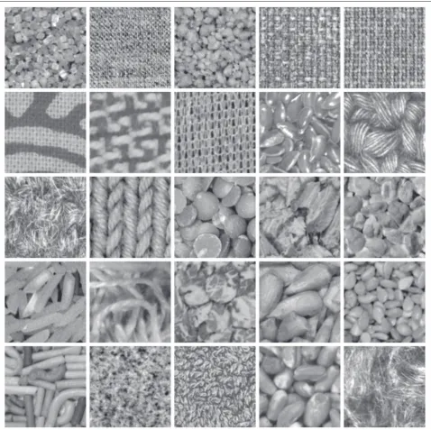
The new dataset contains 25 texture classes, mainly con-sisting of fabrics and arranged textured surfaces using small articles. Figure 1 shows an example patch from each class. The images were acquired using a Canon EOS 550D DSLR camera with a Sigma 17–70-mm zoom lens. The camera was mounted above the textured surfaces, as shown in Fig. 2. Fluorescent lights were placed on two sides of the camera, just above the lens opening. Focus and exposure settings were manually set once for each texture class. The 5184×3456 images were acquired as lossless compressed raw files (CR2). The raw files were corrected for lens distortion, chromatic aberration and vignetting formed by the Sigma lens. The corrections were per-formed according to the settings in the “Adobe (SIGMA 17-70 mm F2.8-4 DC Macro OS HSM, Canon)” lens pro-file in Adobe Photoshop CS5 and then saved as lossless PNG files. The images were next converted to grey scale as 0.2989 R+0.5870 G+0.1140 B, where R, G and B are the red, green and blue intensities, respectively. The selected imaging conditions led to spatially over-sampled images, and to get the textures in a more suitable scale for the rel-atively small local neighbourhoods used in many texture descriptors, the images were sub-sampled to half the orig-inal size (2 592×1 728 pixels) using a Lanczos 3 kernel. By this, the influence of sensor noise was also reduced.
2.1 Hardware rotation
The acquisition setup allows for rotation of the camera around the central axis of the camera lens. By rotating the camera rather than the textured surface, the same light-ing conditions are kept throughout the image acquisition. For each texture class, one image is acquired for each ori-entation. The textures are imaged in the nine orientations θ ∈ {0°, 40°, 80°,. . ., 320°} chosen not to be even multi-ples of 90° for which the choice of interpolation methods would not make a difference.
2.2 Rotation by interpolation
Fig. 1Examples from the 25 texture classes in the Kylberg Sintorn Rotation Dataset. Row 1: cane sugar, canvas, couscous, fabric 1, fabric 2. Row 2: fabric 3, fabric 4, fabric 5, flax seeds, knitwear 1. Row 3: knitwear 2, knitwear 3, lentils, oatmeal, pearl sugar. Row 4: rice, rug, rye flakes, seeds 1, seeds 2. Row 5: sprinkles, floor tile, towel, wheat, wool fur
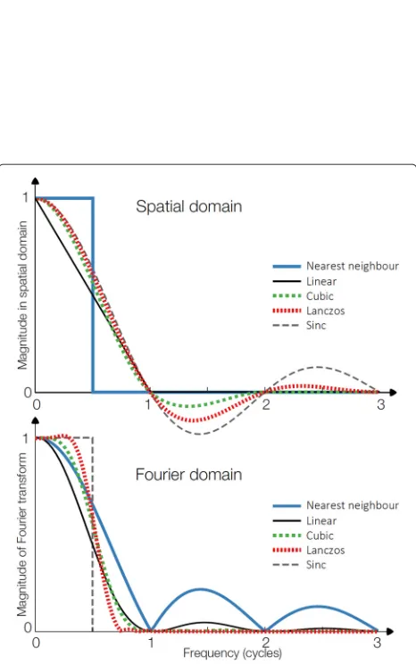
the eight other orientations using each of the interpola-tion approaches. For the interpolainterpola-tion methods based on convolution, Fig. 3 shows 1-D versions of the kernels in spatial as well as in the Fourier domain. The ideal sinc function is also shown for reference. The 1-D definitions of the interpolation methods are as follows:
2.2.1 Nearest neighbour
The interpolation points are assigned the value of the closest pixel:
knearest(x)=
1, |x| ∈[ 0, 0.5] 0, otherwise .
2.2.2 Linear
Assuming a linear transition between pixel intensities gives
klinear(x)=
Fig. 2The texture dataset image acquisition setup. Fromlefttoright: overview, view from the camera towards the texture surface beneath, view from the texture surface towards the camera and lights
Fig. 3Interpolation kernels. 1-D plots of the interpolation kernels and the sinc function in the spatial domain (top) and Fourier domain (bottom)
2.2.3 Cubic
The third order cubic interpolation kernel is a third order polynomial defined as in [15]:
kcubic(x)=
⎧ ⎨ ⎩
3
2|x|3−52|x|2+1, |x| ∈[ 0, 1]
−1
2|x|3+ 52 2
−4|x| +2, |x| ∈(1, 2]
0 otherwise
.
2.2.4 Lanczos
The Lanczos kernel is introduced in [16] and is a win-dowed approximation to the sinc function:
kLanczos(x)=
sinc(x)sinc(x/a), x∈(−a,a)
0 otherwise ,
where
sinc(x)= sin(x)
x ,
and a ∈ Nsets the number of lobes to include of the sinc-function. In this paper, a = 3 is used, resulting in the Lanczos kernel shown in Fig. 3. Interpolation of 2-D signals using Lanczos kernels was introduced in [17].
2.2.5 Spline interpolation
In contrast to the interpolation methods based on con-volution, spline interpolation fits piecewise polynomials between the data points. The interpolated values are then the values the polynomial assumes at the new sample positions. The cubic B-spline interpolation used here, introduced in [18], fits a third order polynomial of the following form:
kBspline(x)=
⎧ ⎨ ⎩
1
2|x|3− |x|2+46, |x| ∈[ 0, 1]
−1
6|x|3+ |x|2−2|x| +86, |x| ∈(1, 2]
0 otherwise
The pieces fit smoothly together, forming a continuous function, going through the original data points.
MATL ABR2012b and the toolbox DIPimage [19] were used for all the interpolations.
2.3 Texture sample generation
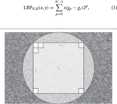
All the images, rotated by hardware and software, are divided into smaller texture samples. The region of an image that is common among the different orientations is a disk centred in the image with the diameter that equals the height of the images (1728 pixels). The largest square within this disk (with the side1 728/√2 = 1 221 ) is divided into 100 sub-squares with a size of 122×122 pixels (since 1 222/10 = 122). The partitioning scheme is illustrated in Fig. 4. Each texture sample is intensity nor-malized to have a mean value of 127 and a standard deviation of 40. The mean is set to be centred in the inter-val [ 0, 255]. The standard deviation is set empirically so that intensity values in the dataset generally do not get mapped to integers∈/[ 0, 255] while retaining most of the dynamic range of the dataset.
3 LBP-based descriptors
In the original definition of LBP [20], the eight connected neighbours of a centre pixel are considered. The neigh-bours are thresholded by the intensity of the centre pixel and placed in a clockwise order producing an 8-bit binary code. The feature vector consists of the occurrences (his-togram) of the different binary codes in a region/patch. The neighbourhood has been generalized to N samples on a radiusRfrom the centre pixel in [8], here denoted LBPN,R. The local binary code for the pixel position(xc,yc) with grey valuegcis defined as:
LBPN,R(x,y)= N−1
p=0
s(gp−gc)2p, (1)
Fig. 4Partitioning scheme. Illustration of the partitioning scheme used to extract texture samples
where
s(x)=
1, x≥0
0, otherwise . (2)
If a pointpdoes not coincide with a pixel centre, linear interpolation is used to compute the grey valuegp. Finally, the histogram of occurring binary codes in a region is the feature vector of this region.
One way of making LBP more robust to noise is to threshold the value of a point, gp with the mean value of the neighbourhood (including the centre pixel),gmean, rather than with the value of the centre pixelgc. The centre pixel is also thresholded with the mean value and included in the binary code. This descriptor is called improved local binary patterns (ILBP) and was introduced in [11]. It is defined as
ILBPN,R(x,y)= N−1
p=0
s(gp−gmean)2p+
+s(gc−gmean)2N, (3)
where
gmean= 1
N+1
⎛ ⎝N−1
p=0 gp+gc
⎞
⎠, (4)
and the functionsis defined as in Eq. 2. Note thatpcis part of the binary code making itN+1 bits long.
In [21], local ternary pattern (LTP) descriptor is pro-posed. The difference between neighbouring valuesgpand the centre pixel valuegc are encoded with three values using a threshold valuet:
s3(gp, gc, t)=
⎧ ⎨ ⎩
1, gp≥gc+t
0, gc−t≤gp<gc+t −1, otherwise
. (5)
In our implementation, as described above, the interval coded with zero is half-bound while in [21] it is open. Instead of using a code with base 3 to encode the three states in Eq. 5, LTP uses two binary codes representing the positive and the negative components of the ternary code, i.e., two binary codes coding for the two states {−1, 1}. These binary codes are collected in two sepa-rate histograms, and as a last step, the histograms are concatenated to form the LTP feature vector [21].
3.1 Rotation invariance
There are different approaches to making the classical LBP descriptor rotation invariant. One way is to group the binary codes that are rotations of one another (i.e. circular shifts of the binary code). Next, the occurrences of each group are computed and used as feature values. This approach is introduced in [8], and the descriptor is denoted LBPriN,R. For example, whenN= 8 is used, there are 36 such rotation invariant groups. Since occurrences of rotation groups are considered, the relative distribu-tion within rotadistribu-tion groups is lost. It also means that the LBPriN,R descriptor achieves rotation invariance by nor-malizing rotation locally, as described in [23].
Another way of making LBP rotation invariant is intro-duced in [9, 23]. The occurrences of rotation codes within the rotation groups are not summed, as in LBPriN,R, but Fourier transformed and the resulting power spectrum is used as the feature vector. The descriptor is called LBP histogram Fourier features (LBPHFN,R). Since the Fourier features are computed on the global histogram of binary codes in the region/patch investigated, LBPHFN,R achieves rotation invariance globally, and hence, retains the rel-ative distribution within rotation groups [23]. However, the LBPHFN,R descriptor in [9] only considers uniform binary codes (binary codes with at the most two tran-sitions between 0 and 1). It was generalized in [10] to include all binary codes, uniform and non-uniform, and called LBPDFT. Together with the LBPDFTdescriptor, the corresponding ILBPDFT descriptor was also introduced in [10].
When having the aforementioned methods at hand, two interesting additional descriptors can be compiled; LTPDFT and ILTPDFT. Thus combining the generalized version of the Fourier features from [10], achieving global rotation invariance, with the promising descriptors LTP from [21] and ILTP from [22].
In the tests reported on here, eight descriptors were used, all with N = 8 samples on a radius R =
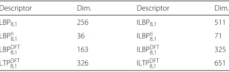
1; LBP8,1, LBPri8,1, LBPDFT8,1 , LTPDFT8,1 , ILBP8,1, ILBPri8,1, ILBPDFT8,1 , ILTPDFT8,1 . The descriptors are listed in Table 1 together with the length of their respective feature vec-tor. The parameters are selected to describe the textures in their highest scale since the effects of interpolation methods are expected to be most prominent here.N =
9 is desirable since the dataset has nine equally spaced
Table 1Texture descriptor dimensionality. Length of feature vector usingN=8
Descriptor Dim. Descriptor Dim.
LBP8,1 256 ILBP8,1 511
LBPri
8,1 36 ILBPri8,1 71
LBPDFT8,1 163 ILBPDFT8,1 325
LTPDFT8,1 326 ILTPDFT8,1 651
orientations and they would otherwise line up perfectly.
N 8 results in feature spaces of very high dimension-ality (e.g. LBPDFT16,1 ∈ R36 883 and ILTPDFT16,1 ∈ R147 532) andN = 8 samples the local neighbourhood atR = 1 well.
4 Classification procedure
The interpolation methods and texture descriptors are evaluated by comparing the obtained classification accu-racies. A first nearest neighbour (1-NN) classifier with Euclidean metric is used. The 1-NN classifier is used to be able to compare classification results obtained on the same and fair basis. To validate the trained classi-fier 10-folded cross-validation is performed by randomly assigning each texture sample an indexn∈ {1, 2,. . ., 10}, creating 10 disjoint subsets with equal number of samples (stratified samples). In the first cross-validation fold, sam-ples withn ∈ {2, 3,. . ., 10}will be the training data and samples withn= 1 will serve as test data. In the second fold, samples withn=2 will be the test data and the rest is used for training, and so on.
The indices for the cross-validation folds are created once and then kept fixed throughout the experiments. The classification results from the 10 folds are combined into a single confusion matrix estimation and the mean and standard deviation of the classification accuracy is computed.
5 Evaluating interpolation methods and rotation invariance
Before the evaluation a baseline is established for each descriptor by training and testing on theθ = 0° orienta-tion. Table 2 lists the means and standard deviations of the classification accuracies of these baseline tests.
The descriptors are applied to all the texture samples, rotated by hardware and by each of the five interpolation methods. For the evaluation, the 1-NN classifier is trained on features from theθ = 0° orientation followed by test-ing on the remaintest-ing eight orientations, one by one. The results are shown in Fig. 5. The established baselines are shown as dashed red lines in Fig. 5. One dot in Fig. 5 corresponds to one classification test where the classi-fier has been trained on θ = 0° orientation and tested on one of the remaining orientations (using 10-folded cross-validation).
Table 2Mean classification accuracy atθ=0°. Standard deviations in brackets
Descriptor Mean Std. Descriptor Mean Std.
LBP8,1 96.4 (1.2) ILBP8,1 95.4 (0.9)
LBPri
8,1 97.2 (0.9) ILBPri8,1 96.9 (0.9)
LBPDFT8,1 98.7 (0.7) ILBPDFT8,1 97.5 (0.7)
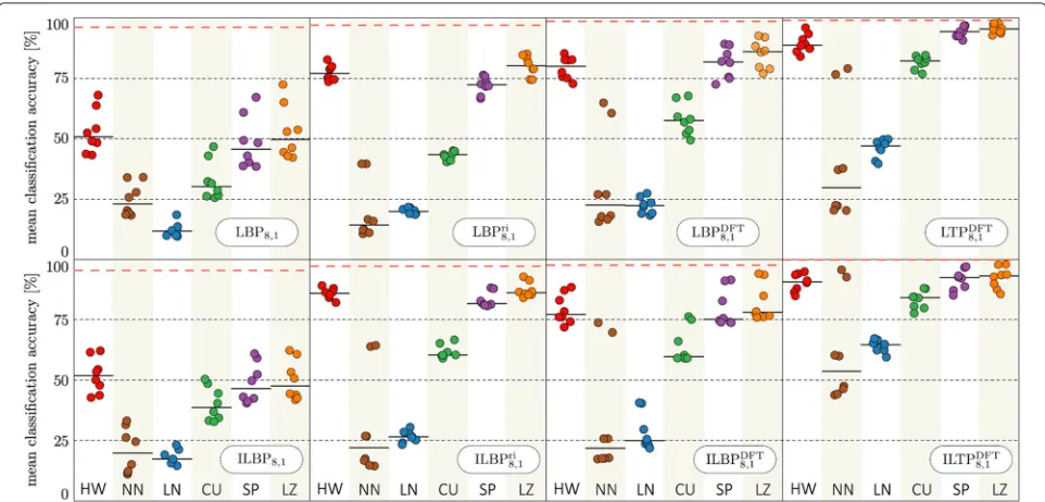
Fig. 5Rotation invariance test. Plot of mean classification accuracies (in %) when training on theθ=0° orientation and testing onθ∈ {40°, 80°,. . . 320°}for each descriptor applied on textures rotated by hardware (HW) or nearest neighbour (NN), linear (LN), cubic (CU), B-spline (SP) and Lanczos 3 (LZ) interpolation. Thehorizontal red dashed linesare the mean accuracies when training and testing onθ=0°. Each dot corresponds to the mean classification accuracy from one rotation test. Theblack horizontal line segmentsin each column mark the median in each distribution
5.1 Interpolation method
Figure 5 shows that the obtained classification accura-cies differ greatly for the different interpolation methods (Additional file 1). This indicates that the characteristic properties of the textures are retained to a widely varying degree under rotation. Lanczos and B-spline interpolation results in accuracies similar to, or even better than, that of the hardware rotated textures. Nearest neighbour, lin-ear and cubic interpolation all show lower accuracies for all descriptors compared.
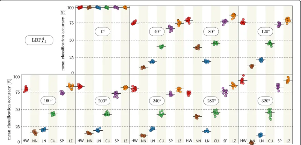
For the nearest neighbour rotated textures, some rota-tion tests (dots in Fig. 5) show relatively high accuracies for several descriptors. To investigate this, Fig. 6 shows the result for the LBPri8,1descriptor in more detail. Here, each dot is a cross-validation fold in a rotation test. It can be seen that the nearest neighbour has noticeably higher accuracies atθ = 80° andθ = 280°. These two angles correspond to the two dots that often have higher accura-cies than the rest for the nearest neighbour interpolation method in Fig. 5. Rotations of a digital image with even multiples of 90° are ideal/lossless. The two orientations of the texturesθ ∈ {80°, 280°}in the dataset are the two that are closest to even multiples of 90° and, hence, closest to ideal rotations for which nearest neighbour is relatively successful.
In a few cases, the result achieved using Lanczos and B-spline interpolation exceeds the result obtained using the hardware rotated textures, especially atθ ∈ {80°, 280°}, see
Fig. 6. This can, to a certain degree, be explained by that, in the case of hardware rotations, the sensor noise is sam-pled again and again for the different orientations, while the interpolated images all originate from one image with the sensor noise sampled once. The set of images which are rotated by interpolation is hence more homogeneous, and in addition, these two orientations are closest to ideal orientations of the original image, as was discussed above with respect to the higher performance for near-est neighbour interpolation for those two angles. Another explanation can be found by studying the per-class accu-racies (data not shown). The classifier runs into problems with class number 12 and 20 for the hardware rotated tex-tures while they are easier to classify in the Lanczos and B-spline interpolated data.
Fig. 6Rotation invariance test for LBPri
8,1in detail. Plot of mean classification accuracies within each cross-validation fold for each orientation for the LBPri
8,1descriptor applied on textures rotated by hardware (HW) or nearest neighbour (NN), linear (LN), cubic (CU), B-spline (SP) and Lanczos 3 (LZ) interpolation. Theblack horizontal line segmentsin each column mark the median in each distribution
5.2 Rotation invariance
The rotation invariance of the descriptors can be eval-uated in Fig. 5. Mean and standard deviation is also reported in Table 3. A truly rotation invariant texture descriptor should only show subtle variations over differ-ent oridiffer-entations of a texture. The classic LBP has obvious problems in the rotation tests and fall far below the base-line. The LBP-versions design to be rotation invariant do achieve higher accuracies than the classic LBP. However, none of the descriptors reach their baseline accuracy.
Figure 6 shows that the cross-validation folds give very similar results. This means that the standard deviations over orientations, see Fig. 5, are not due to inadequate validation of the classifier but a genuine variation in descriptor performance.
5.2.1 Reference methods
To put the rotation invariance of the LBP-based descrip-tor into perspective, three additional descripdescrip-tors were
Table 3Mean classification accuracy (and standard deviations in brackets) across the eight rotation tests. A rotation test refers to training onθ=0° and testing on one of the other rotations
θ=0°
Descriptor Mean Std. Descriptor Mean Std.
LBP8,1 52.9 (8.9) ILBP8,1 52.0 (7.3)
LBPri
8,1 77.4 (3.2) ILBPri8,1 85.9 (2.2)
LBPDFT8,1 79.3 (4.6) ILBPDFT8,1 79.4 (6.1)
LTPDFT8,1 89.5 (3.9) ILTPDFT8,1 90.4 (3.7)
evaluated in the same way. The rotation invariant Gabor filter bank achieved a mean accuracy over rotation tests of 90.4 %, Haralick features 75.3 % and MR8 56.6 %. These values should be compared to the mean classi-fication accuracies reported in Table 3 (also showed as black lines in Fig. 5). The Gabor filter bank achieves as good results as the best descriptor tested in the LBP family
ILTPDFT8,1
while Haralick achieves just below the local rotation invariant LBPr8,1i descriptor. Below fol-lows condensed details of how the reference methods were used.
For the Gabor filter bank, definitions and guidelines as described in [7, 24] were used. The frequency ratio was set to√2, the number of orientations was set to eight, and the number of frequencies to six. The Gaussian envelope was set to(γ,η) = (3, 2), and the kernel size was set to 19×19.
The Haralick features were defined and used as described in [25]. The contrast, correlation, energy and homogeneity measures were computed for four grey-level co-occurrence matrices (four directions) using quantization into 16 grey levels and a distance of two pixels.
MR8 was defined and used as in [26].
6 Computational cost
Fig. 7Computational cost for the different interpolation methods. The costs are given relative to linear interpolation
6.1 Interpolation methods
The computational time was measured while rotating the 2500 texture samples to the eight orientations. Figure 7 shows the computation time relative to rotating the tex-ture sample using linear interpolation. The two best performing interpolation methods (in terms of retain-ing texture information) are slightly more computationally expensive; a factor of 1.27 for Lanczos and 1.45 for Spline.
6.2 Texture descriptors
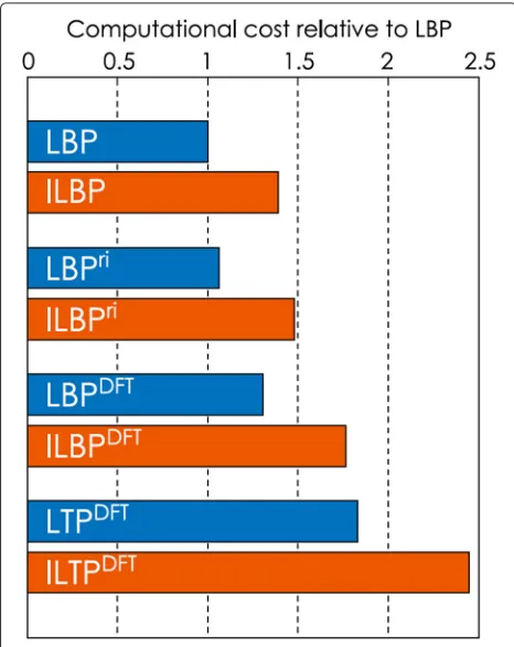
The computational time for the different descriptors was measured while applying them to the 2500 texture sam-ples of the 0° orientation. Figure 8 shows the computation
Fig. 8Computational cost for the texture descriptors. The costs are given relative to the LBP descriptor
time relative to the LBP descriptor. The slowest descrip-tor is the ILTPDFTbeing about 2.5 times slower than LBP. However, all the descriptors in the LBP family evaluated in this manuscript are computationally cheap compared to the filter-based texture descriptors used here as ref-erence methods. The Gabor filter bank takes about 37 times as long to compute as the basic LBP. The numbers may vary with implementations and systems but convolv-ing the texture sample with a whole bank of filter kernels is more computationally expensive than computing these LBP-variants.
7 Rotation representation in classification
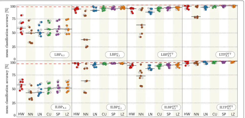
Fig. 9Rotation invariance when training on two orientations. Plot of mean classification accuracies (in %) when training on the two orientationsθ∈ {0°, 40°}and testing onθ∈ {80°, 120°,. . .320°}for each descriptor applied on textures rotated by hardware (HW) or nearest neighbour (NN), linear (LN), cubic (CU), B-spline (SP) and Lanczos 3 (LZ) interpolation. The horizontalred dashed linesare the mean accuracies when training and testing onθ=0°. Thegrey dots in the background correspond to the mean classification accuracies achieved when the size of the training data is halved. Thehorizontal line segmentsmark the median in each distribution
representation of the rotated textures rather than a larger training set, we carried out a complementary test where every other sample was removed from the training set, making it the same size as in the previous tests. These results are shown as grey dots in the background in Fig. 9 and prove that the improvement is not from an increase in the number of training samples.
Figure 10 shows how the classification accuracies change when even more orientations are used in the train-ing data, rangtrain-ing from one (as in the evaluation reported on in Section 4) to eight orientations. The additional ori-entations are the Lanczos interpolated data, following the scenario of adding “artificial” samples to the training data. It shows that the introduction of a second orientation in the training data is very beneficial in terms of tex-ture recognition. For the less rotation invariant textex-ture descriptors, additional orientations (more than two) fur-ther improve the classification accuracies even though the achieved accuracies level out and do not reach the levels of the rotation invariant descriptors. This trend is not as clear for the more rotation invariant descriptors, for which a third and fourth orientation only improves the classifi-cation accuracies slightly. Overall, ILTPDFT8,1 and LTPDFT8,1 are found at the top with mean accuracies between 99 and 100 % when at least four orientations are included in the training data.
8 Conclusions
Based on the performed experiments we conclude that
• Lanczos 3 interpolation, closely followed by B-splines outperform the other interpolation strategies in all tests. The same levels of texture recognition are achieved using these two interpolation methods as those using hardware-rotated textures.
• As expected, the interpolation methods closer to the ideal sinc function retain the texture information best. The commonly used linear and cubic interpolation clearly have shortcomings in preserving texture information in the setting of texture recognition. • The best performing interpolation methods are only
slightly more computationally expensive. Lanczos stands out as it is both the best interpolation method in terms of preserving texture information and faster to compute than the second best interpolation method B-spline.
• Both the local rotation invariant versions (by counting occurrences of rotation groups), and the global rotation invariant versions (by computing Fourier descriptors of the groups) of the LBP-based texture descriptors are less rotation variant than the classic LBP descriptor but they still suffer from rotation variance.
• TheLTPDFTandILTPDFTdescriptors perform better than the other tested descriptors. They both show high classification accuracies and low standard deviations over different orientations.
• TheILTPDFTachieves the same high classification accuracy as an optimized and rotation invariant Gabor filter bank. The other reference descriptors are inferior to all the tested rotation invariant forms of the LBP descriptors.
• Even though the more advanced descriptors in the LBP family are more computationally expensive than the basic LBP, they are all computationally
inexpensive compared to common filter bank-based texture descriptors such as Gabor filter banks and MR8.
• Including several different orientations of the textures in the training data has great positive impact on the classification accuracies. This also
compensates to a large extent the shortcomings of choosing a simple interpolation method. Hence, a simple strategy that should be generally considered!
Linear and cubic interpolation is still commonly used even though they are easily outperformed in terms of retaining texture information. For example, in the image processing software ImageJ, linear interpolation is the default, in GIMP cubic is default (although Lanzos 3 is offered as an option) and MATL ABonly supports nearest neighbour, linear and cubic interpolation when rotating images. The software library OpenCV has linear interpo-lation as default while cubic is optional.
Furthermore, these tests show that the use of rotation invariant texture descriptors may not be enough to achieve rotation invariant texture recognition; represent-ing different orientations of the textures in the train-ing data shows to be very important, even if the extra
orientations are artificially generated by rotating already existing samples by means of interpolation.
In the light of these findings, the use of linear interpola-tion to compute the intensity samples in the local neigh-bourhoods in all the LBPN,R-based descriptors should perhaps be revised.
Additional file
Additional file 1:Tables for the data illustrated in Figs. 5 and 7. (PDF 108 kb)
Competing interests
The authors do not have any competing interests.
Authors’ contributions
Both authors have contributed equally to the text while GK have implemented the texture descriptors and performed most of the tests.
Acknowledgements
The authors would like to thank Cris Luengo for expanding the set of interpolation kernels implemented in DIPimage. This work has been part of the MiniTEM E!6143 project funded by EU and EUREKA through the Eurostars Programme.
Received: 22 June 2015 Accepted: 17 March 2016
References
1. X Tan, B Triggs, Enhanced local texture feature sets for face recognition under difficult lighting conditions. IEEE Trans. Image Process.19(6), 1635–1650 (2010)
2. K Jafari-Khouzani, H Soltanian-Zadeh, Radon transform orientation estimation for rotation invariant texture analysis. IEEE Trans. Pattern Anal. Mach. Intell.27(6), 1004–1008 (2005)
3. B Schölkopf,Support vector learning. (PhD thesis, Technische Universität Berlin, 1997)
4. J Zhang, T Tan, Brief review of invariant texture analysis methods. Pattern Recogn.35(3), 735–747 (2002)
5. Y Xu, H Ji, C Fermüller, Viewpoint invariant texture description using fractal analysis. Int. J. Comput. Vis.83(1), 85–100 (2009)
6. M Varma, A Zisserman, A statistical approach to texture classification from single images. Int. J. Comput. Vision.62(1-2), 61–81 (2005)
7. F Bianconi, A Fernández, A Mancini, inProceedings of the 20th International Congress on Graphical Engineering. Assessment of rotation-invariant texture classification through gabor filters and discrete Fourier transform (ACM, Valencia, Spain, 2008)
8. T Ojala, T Mäenpää, Multiresolution Gray-Scale and Rotation Invariant Texture Classification with Local Binary Patterns. IEEE Trans. Pattern Anal. Mach. Intell.24(7), 971–987 (2002)
9. T Ahonen, J Matas, C He, M Pietikäinen, inProceedings of the 16th Scandinavian Conference on Image Analysis. LNCS. Rotation invariant image description with local binary pattern histogram Fourier features, vol. 5575 (Springer, Berlin Heidelberg, 2009), pp. 61–70
10. A Fernández, O Ghita, E González, F Bianconi, PF Whelan, Evaluation of robustness against rotation of LBP, CCR and ILBP features in granite texture classification. Mach. Vis. Appl.22(6), 913–926 (2011) 11. H Jin, Q Liu, H Lu, X Tong, inProceedings of the Third International
Conference on Image and Graphics. Face detection using improved LBP under Bayesian framework, (IEEE Computer Society, Washington, DC, USA, 2004), pp. 306–309. doi:10.1109/ICIG.2004.62
12. A Fernández, M Álvarez, F Bianconi, Texture description through histograms of equivalent patterns. J. Math. Imaging Vis.45, 76–102 (2013) 13. G Kylberg, I-M Sintorn, Kylberg Sintorn Rotation dataset (2015). http://
14. T Ojala, T Mäenpää, M Pietikäinen, J Viertola, J Kyllönen, S Huovinen, in Proceedings of the 16th International Conference on Pattern Recognition, Quebec, Canada. Outex - New Framework for Empirical Evaluation of Texture Analysis Algorithms (IEEE Computer Society, Washington, DC, USA, 2002), pp. 701–706
15. R Keys, Cubic convolution interpolation for digital image processing. IEEE Trans. Acoust. Speech Signal Process.29(6), 1153–1160 (1981)
16. C Lanczos,Applied Analysis. Prentice-Hall mathematics series. (Prentice-Hall, New Jersey, 1956)
17. CE Duchon, Lanczos Filtering in One and Two Dimensions. J. Appl. Meteor.18(8), 1016–1022 (1979)
18. H Hou, H Andrews, Cubic splines for image interpolation and digital filtering. IEEE Trans. Acoust. Speech Signal Process.26(6), 508–517 (1978) 19. C Luengo, DIPimage, a Matlab toolbox for scientific image processing
and analysis. http://www.diplib.org/. Accessed 1 Jan 2016 20. T Ojala, M Pietikäinen, D Harwood, A comparative study of texture
measures with classification based on featured distributions. Pattern Recogn.29(1), 51–59 (1996)
21. X Tan, B Triggs, inAnalysis and Modeling of Faces and Gestures. Lecture Notes in Computer Science, ed. by SK Zhou, W Zhao, X Tang, and S Gong. Enhanced local texture feature sets for face recognition under difficult lighting conditions, vol. 4778 (Springer, Springer-Verlag Berlin Heidelberg, 2007), pp. 168–182
22. L Nanni, S Brahnam, A Lumini, A local approach based on a Local Binary Patterns variant texture descriptor for classifying pain states. Expert Syst. Appl.37(12), 7888–7894 (2010)
23. G Zhao, T Ahonen, J Matas, M Pietikainen, Rotation-invariant image and video description with local binary pattern features. IEEE Trans. Image Process.21(4), 1465–1477 (2012)
24. F Bianconi, A Fernández, Evaluation of the effects of Gabor filter parameters on texture classification. Pattern Recog.40(12), 3325–3335 (2007)
25. RM Haralick, K Shanmugam, I Dinstein, Textural Features for Image Classification. IEEE Trans. Syst. Man Cybern.3(6), 610–621 (1973) 26. M Varma, A Zisserman, inProceedings of the 7th European Conference on
Computer Vision, Copenhagen, Denmark. Computer Vision. Classifying images of materials: Achieving viewpoint and illumination independence, vol. 3 (Springer, Berlin, 2002), pp. 255–271
Submit your manuscript to a
journal and benefi t from:
7Convenient online submission 7Rigorous peer review
7Immediate publication on acceptance 7Open access: articles freely available online 7High visibility within the fi eld
7Retaining the copyright to your article