Comparison of varieties of numerical methods applied to lid-driven cavity flow: coupling algorithms, staggered grid vs. collocated grid, and FUDS vs. SUDS

O R I G I N A L P A P E R

Open Access

Comparison of varieties of numerical

methods applied to lid-driven cavity flow:

coupling algorithms, staggered grid vs.

collocated grid, and FUDS vs. SUDS

A. A. Boroujerdi

and M. Hamzeh

Abstract

The effectiveness of different methods, schemes, algorithms, and approaches is of substantial challenging problems in numerical modeling of transport phenomena. In the present paper, a lid-driven cavity problem is modeled via two basically different approaches of spatial discretization: collocated and staggered. The non-dimensionalized governing equations are semi-discretized by using a finite volume approach. Then, the full discretization is performed in each of collocated and staggered grids, separately. Upwind and central difference schemes are implemented in order to discretize the convective and diffusion terms of equations, respectively. After mesh independency study, the performances of collocated and staggered grids in comparison with the reference benchmark are presented. Next, the effectiveness of the first and the second order upwind schemes are presented, as well as different coupling algorithms of SIMPLE, SIMPLEC, and SIMPLER. Finally, an overall comparison of the methods is provided and acceptable agreements with benchmark are attained.

Keywords:Numerical simulation, Collocated, Staggered, Lid-driven cavity, Upwind scheme, Coupling algorithm

Introduction

As a classic problem, lid-driven cavity flow is widely imple-mented in order to validate, compare, and investigate nu-merical methods and schemes.

Staggered gridhas been extensively used for the numer-ical modeling of lid-driven cavity flows. A two-dimensional computational model was developed to study the fluid dy-namic behavior in a square cavity driven by an oscillating lid using staggered grid-based finite volume method (Indu-kuri and Maniyeri,2018). The numerical simulations were performed for the case of top wall oscillations for various combinations of Reynolds number and frequencies. From these simulations, an optimum frequency was chosen and then the vortex behavior for the cases of parallel wall os-cillations was explored. McDonough (2007) investigated lid-driven cavity problem by use of a new form of large-eddy simulation at moderate Reynolds number to demon-strate the ability of the procedure to automatically predict

transition to turbulence. They reported parallel speedups observed on a general-purpose symmetric multiprocessor employing MPI for parallelization. Gutt and Groşan (2015) analyzed the motion of an incompressible viscous fluid through a porous medium located in a two-dimensional square lid-driven cavity flow described by a generalized Darcy–Brinkman model. The effect of inertia and rheology parameters on the flow of viscoplastic fluids inside a lid-driven cavity is investigated using a stabilized finite element approximation (dos Santos et al. 2011). Patil, Lakshmisha, and Rogg (2006) presented the results for deep cavities with aspect ratios of 1.5–4, and Reynolds numbers of 50–3200. Several features of the flow, such as the location and strength of the primary vortex, and the corner-eddy dynamics were investigated and compared with previous findings from experiments and theory.

Direct numerical simulations about the transition process from laminar to chaotic flow in square lid-driven cavity 2D incompressible flow with increasing Reynolds numbers flows were considered by (Peng, Shiau, and Hwang, 2003). The spatial discretization consisted of a

© The Author(s). 2019Open AccessThis article is distributed under the terms of the Creative Commons Attribution 4.0 International License (http://creativecommons.org/licenses/by/4.0/), which permits unrestricted use, distribution, and reproduction in any medium, provided you give appropriate credit to the original author(s) and the source, provide a link to the Creative Commons license, and indicate if changes were made.

* Correspondence:[email protected]

seventh-order upwind-biased method for the convection term and a sixth-order central method for the diffusive term.

Collocated grid arrangement is also implemented in order to simulate lid-driven cavity flows. Peng (Ding,

2017) employed the SIMPLE algorithm and its variants to solve the driven-cavity problem at Re < 10,000 by propos-ing a new segregated solver for determinpropos-ing the solution of incompressible flow on structured collocated grid sys-tems. Case studies of steady incompressible flow in a 2D lid-driven square cavity were investigated for 100 < Re < 5000 by AbdelMigid et al. (Tamer, Khalid, Mohamed, and Ahmed,2017). Collocated grid arrangement along with a uniform structured Cartesian grid was used. Yapici, Kara-sozen, and Uludag (2009) presented a finite volume tech-nique for the numerical solution of steady laminar flow of Oldroyd-B fluid in a lid-driven square cavity over a wide range of Reynolds and Weissenberg numbers. Second-order central difference (CD) scheme was used for the convection part of the momentum equation while first-order upwind approximation was employed to handle viscoelastic stresses. In another work, a numerical collo-cated finite volume method was presented to study Buon-giorno’s nanofluid model for MHD mixed convection of a lid-driven cavity filled with nanofluid (Elshehabey and Ahmed,2015).

Methods

Aim and design for the study

The principal aim of the following research is to compare different computational methods for simulation of a cavity fluid flow driven by a moving lid and to introduce appro-priate schemes. The model is based on the finite volume method of the governing equation semi-discretization in two over ally different formulations of staggered and col-located grid systems. The full discretization is made by both the first-order and the second-order upwind schemes. Three different coupling algorithms of SIMPLE, SIMPLEC, and SIMPLER are developed. Afterward, the results of all the methods are compared.

Description of the methodology

Semi-discretization of governing equations

The physical and computational domains of the problem area square cavity with the dimensions ofLwhose upper lid is moving rightward with the velocity of u0. The ori-gin of the Cartesian coordinate is located at the left lower corner of the cavity.

In order to simplify the model, we consider the follow-ing assumptions:

1) Working fluid is incompressible.

2) The shear stress tensor is proportional to the deformation rate (Newtonian fluid)

3) There are no external body forces. 4) The flow is laminar.

The governing equations are continuity and momentum equations, which for a steady laminar flow of incompress-ible fluid with constant viscosity and no external force are as follows:

∂u ∂xþ

∂v

∂y¼0 ð1Þ

∂ ∂x u

2

þ_∂∂ y u

_v

ð Þ ¼−_ρ1∂_∂P

x

þμ_ρ ∂_∂2u x2þ

∂2 u ∂y2

ð2Þ

∂ ∂x u

_v

ð Þ þ ∂

∂y v

2 _¼−1

ρ ∂P ∂y þμ

ρ ∂2_v ∂x2þ

∂2_v ∂y2

ð3Þ

Making governing equations non-dimensional enables us to incorporate some fluid and geometric parameters and to generalize the results of the simulation. We scale thexandycoordinates by the dimension of cavityL, the velocities by lid velocity, and pressure by dynamic pres-sure as described below:

x¼x

L ; y¼ y L ; u¼

u

u₀ ; v¼ v u₀ ;

P¼ P _−P 0 1 2ρ _u 0 2 ð4Þ

Substituting the definitions, one can attain non-dimensionalized equations:

∂u ∂xþ

∂v

∂y¼0 ð5Þ

∂ ∂x u

2 _þ ∂

∂yð Þ ¼uv − ∂P ∂xþ

1 Re

∂2 u ∂x2þ

∂2 u ∂y2

ð6Þ

∂ ∂xð Þ þuv

∂ ∂y v

2 _¼−∂P

∂yþ 1 Re

∂2_v

∂x2þ

∂2_v

∂y2

ð7Þ

Re¼ρ _u

0L

μ ð8Þ

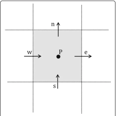
The next step is to discretize the computational do-main. Whether the grid system is collocated or stag-gered, integrating governing Eqs. (5)–(7) over an arbitrary control volume depicted in Fig. 2 gives semi-discretized Eqs. (9)–(11).

Aeu^e−Aw^uw

½ þ½An^vn−As^vs ¼0 ð9Þ

Aeu^eue−Aw^uwuw

½ þ½An^vnun−As^vsus

¼−∂_∂P

x

P

APΔxP

þ 1 Re Ae

∂u ∂x

e

−Aw∂

u ∂x

w

þAn∂

u ∂y

n

−As∂

u ∂y s

ð10Þ

An^vnvn−As^vsvs

½ þ½Ae^ueve−Aw^uwvw

¼−∂_∂P

y

P

APΔyP

þ 1 Re Ae

∂v ∂x

e

−Aw∂

v ∂x

w

þAn∂

v ∂y

n

−As∂

v ∂y s

ð11Þ

The velocities with that are convecting velocities, which convey mass or momentum of fluid parcels. Con-sidering uniform Cartesian grid and Δx=Δy, divide the last three equations by cross-sectional area, we have

^

ue−^uw

½ þ½^vn−^vs ¼0 ð12Þ

^

ueue−^uwuw

½ þ½^vnun−^vsus

¼ðPw−PeÞ þ

1 Re ∂u ∂x e

−∂_∂u

x

w

þ∂_∂u y

n

−∂_∂u

y s ð13Þ ^

vnvn−^vsvs

½ þ½^ueve−^uwvw

¼ðPs−PnÞ þ

1 Re ∂v ∂x e

−∂_∂v

x

w

þ∂_∂v y

n

−∂_∂v

y

s

ð14Þ

The above equations govern all the control volumes and are applicable for both collocated and staggered grid. In the following section, the discretization of the equations for the collocated and staggered grid will be presented in details.

Discretization in staggered grid

The schematic of staggered grid arrangement is depicted in Fig. 2. Apparently, the u, v, and scalar (pressure) control volumes are staggered with respect to each other. Firstly, consider x-momentum Eq. (13) for non-boundary u-control volumes shown in Fig. 2. Approximate the diffusion terms of viscous stresses by central difference scheme.

^

ueue−^uwuw

½ þ½^vnun−^vsus ¼ðPw−PeÞ

1

ΔxRe½ðuE−uPÞ−ðuP−uWÞ þðuN−uPÞ

−ðuP−uSÞ

ð15Þ

Approximate convecting velocities by the central lin-ear scheme as follows:

^

ue¼

uPþuE

2 ¼

ui;Jþuiþ1;J

2 ð16Þ

^

uw¼

uWþuP

2 ¼

ui−1;Jþui;J

2 ð17Þ

^vn¼

vI−1;jþvI;j

2 ð18Þ

^vs¼

vI−1;jþ1þvI;jþ1

2 ð19Þ

The upwind scheme is implemented for convected vel-ocities. In order to generalize the formulation, the rela-tion is derived for the second order upwind. The scheme can be simply changed to the first order upwind only by setting the coefficients 1.5 and 0.5 to 1.0 and 0.0 respectively.

^

ueue¼ ½1:5 maxðu^e;0ÞuP −0:5 maxð^ue;0ÞuW

−½1:5 maxð−^ue;0ÞuE−0:5 maxð−^ue;0ÞuEE

ð20Þ

^

uwuw¼ ½1:5 maxðu^w;0ÞuW −0:5 maxð^uw;0ÞuWW

−½1:5 maxð−^uw;0ÞuP−0:5 maxð−^uw;0ÞuE

ð21Þ

Note that at the vertex points (s and n for x

-mo-mentum and w and e for y-momentum), term uv is

approximated by central difference scheme as

^vnun¼^vn

uPþuN

2 ð22Þ

^vsus¼^vs

uSþuP

2 ð23Þ

The pressure force exerted on the faces of u-control volume does not need to be approximated because the faces of u-control volume coincide with pressure node, so that

Pw−Pe

ð Þ ¼ PI−1;J−PI;J

ð24Þ

Performing the aforementioned approximations forx -momentum equation, we attained the following algebraic linear equation based on the central node and neighbor-ing node values ofu-velocity.

aPuP¼aWWuWW þaWuWþaEuEþaEEuEE

þaSuSþaNuNþ PI−1;J−PI;J

ð25Þ

The Eq. (25) whose coefficients are as follows governs all the control volumes except for boundary volumes.

aP¼1:5 maxðu^e;0Þ þ1:5 maxð−^uw;0Þ

þð^vn−^vsÞ

2 þ

4

ΔxRe ð26Þ

aWW ¼−0:5 maxðu^w;0Þ ð27Þ

aW ¼0:5 maxðu^e;0Þ þ1:5 maxð^uw;0Þ þ

1

ΔxRe ð28Þ

aE¼1:5 maxð−^ue;0Þ þ0:5 maxð−^uw;0Þ

þ_Δ1

xRe ð29Þ

aEE¼−0:5 maxð−^ue;0Þ ð30Þ

aS ¼ ^

vs

2þ

1

ΔxRe ð31Þ

aN ¼−^

vn

2 þ

1

ΔxRe ð32Þ

The boundary conditions of x-momentum equation

are

Near left wall: for the first column of half-volumes whose centers located atx= 0, the no-penetration condi-tion must be satisfied.

uP≡ui;J ¼0 i¼1 ; J¼1 to n ð33Þ

For the second column of volumes, in the second-order upwind scheme, uww does not exist, so the equa-tions must be modified based on the first order upwind as follows:

^

uwuw¼½maxð^uw;0ÞuW

−½1:5 maxð−^uw;0ÞuP−0:5 maxð−^uw;0ÞuE

i¼2 ; J ¼1 to n ð34Þ

Near right wall: for the last column of half-volumes whose centers are located atx= 1, no-penetration condi-tion must be satisfied.

uP≡ui;J ¼0 i¼nþ1 ; J

¼1 to n ð35Þ

For one to the last column of volumes, the discretization scheme must be amended.

^

ueue¼ ½1:5 maxð^ue;0ÞuP−0:5 maxðu^e;0ÞuW

−½maxð−^ue;0ÞuE

i¼n ; J ¼1 to n ð36Þ

Lower wall control volumes (the first row), i.e., in the vicinity of y= 0: in these volumes, the viscous term of ∂u/∂y must be approximated by forward scheme rather than central scheme.

∂u ∂y

s

¼ðu_ΔP−0Þ

y=2 ð37Þ

WhereUy= 0is the velocity of the lower wall. Similarly, for the upper wall at the vicinity of y= 1 the viscous

term of ∂u/∂y must be approximated by backward

scheme rather than central scheme

∂u ∂y

n

¼ðu0−uPÞ

Δy=2 ð38Þ

For four corners, a combination of the mentioned boundary conditions must be used.

Similarly, consider y-momentum Eq. (14) for

discretize diffusion terms for those CVs, we use the CDS.

^

vnvn−^vsvs

½ þ½^ueve−^uwvw

¼ðPs−PnÞ

1

ΔxRe½ðvE−vPÞ−ðvP−vWÞ

þðvN−vPÞ−ðvP−vSÞ ð39Þ

Approximate convecting velocities at four faces by

CDS.

^

ue¼

uiþ1;J−1þuiþ1;J

2 ð40Þ

^

uw¼

ui;J−1þui;J

2 ð41Þ

^vn¼

vPþvN

2 ¼

vI;jþvI;jþ1

2 ð42Þ

^vs¼

vSþvP

2 ¼

vI;j−1þvI;j

2 ð43Þ

The convected velocities at vertical faces are discre-tized by the second-order upwind scheme. To alter the scheme to the first order, the coefficients 1.5 and 0.5 should be changed to 1.0 and 0.0 respectively.

^

vnvn¼ ½1:5 maxð^vn;0ÞvP −0:5 maxð^vn;0ÞvS

−½1:5 maxð−^vn;0ÞvN−0:5 maxð−^vn;0ÞvNN

ð44Þ

^

vsvs¼ ½1:5 maxðv^s;0ÞvS −0:5 maxð^vs;0ÞvSS

−½1:5 maxð−^vs;0ÞvP−0:5 maxð−^vs;0ÞvN

ð45Þ

Note that at the vertex pointsw and e, the termuvis approximated by central difference scheme as follows:

^

ueve¼u^e

vPþvE

2 ð46Þ

^

uwvw¼^uw

vWþvP

2 ð47Þ

The pressures at vertical faces coincide with their nodal points as follows:

Ps−Pn

ð Þ ¼ PI;J−1−PI;J

ð48Þ

The final form of discretized y-momentum equation

based on central and neighboring node values is as follows:

aPvP¼aSSvSSþaSvSþaNvNþaNNvNN

þaWvWþaSvSþ PI;J−1−PI;J

ð49Þ

The above equation dominates all the v-velocity CVs except for boundaries. The relations of the coefficients for the second order upwind are

aP¼1:5 maxðv^n;0Þ þ1:5 maxð−^vs;0Þ

þð^ue−^uwÞ

2 þ

4

ΔxRe ð50Þ

aSS ¼−0:5 maxð^vs;0Þ ð51Þ

aS ¼0:5 maxðv^n;0Þ þ1:5 maxð^vs;0Þ þ

1

ΔxRe ð52Þ

aN ¼1:5 maxð−^vn;0Þ þ0:5 maxð−^vs;0Þ

þ_Δ1

xRe ð53Þ

aNN ¼−0:5 maxð−^vn;0Þ ð54Þ

aW ¼^

uw

2 þ

1

ΔxRe ð55Þ

aE¼−^

ue

2 þ

1

ΔxRe ð56Þ

Boundary conditions of y-momentum equation are as

follows:

Near the bottom wall: the no-penetration condition must be satisfied for the first row.

vP≡vI;j¼0 j¼1 ; I¼1 to n ð57Þ

For the second row of v-velocity CVs, the

second-order upwind must be replaced by the first one at posi-tive flow.

vsvs¼½maxð^vs;0ÞvS−½1:5 maxð−v^s;0ÞvP−0:5 maxð−v^s;0ÞvNj

¼2 ; I¼1 to n

ð58Þ

vP≡vI;j¼0 j¼nþ1 ; I

¼1 ton ð59Þ

For one to the last CV, the negative flow direction must be approximated by the first-order upwind.

^

vnvn¼ ½1:5 maxð^vn;0ÞvP−0:5 maxð^vn;0ÞvS −½ maxð−v^n;0ÞvN

j¼n ; I¼1 to n

ð60Þ

In the leftmost CVs (nearx= 0), use forward difference scheme instead of CDS for discretization of viscous stress as ∂v ∂x w

¼ð_ΔvP−0Þ

x=2 ð61Þ

WhereVx= 0is the left wall velocity.

For the rightmost CVs (near x= 1), implement the

backward scheme to discretize the diffusion term.

∂v ∂x

e

¼ð0−vPÞ

Δx=2 ð62Þ

At four corners of the computational domain, a com-bination of the described boundary conditions must be utilized.

In order to implement the family of SIMPLE algo-rithms, manipulate the continuity equation to attain an algebraic equation in terms of nodal pressures to use in couple with the momentum equations.

ue−uw

½ þ½vn−vs ¼0 ð63Þ

The velocities at the faces of scalar CVs are their nodal values so

uiþ1;J−ui;J

þ vI;jþ1−vI;j

¼0 ð64Þ

According to the SIMPLE algorithm, the first step is to guess the pressure field. Nevertheless, due to the non-linearity of the momentum equation, the velocity field must be guessed also. Consider the discretized momen-tum equations for exact solutionuand approximate so-lutionu*:

aPuP¼ X

anbunbþ PI−1;J−PI;J

ð65Þ

aPuP¼ X

anbunbþ PI−1;J−PI;J

ð66Þ

Subtracting the last two equations gives

aP uP−uP

¼Xanb unb−unb

þ PI−1;J−PI−1;J

− PI;J−PI;J

h i

ð67Þ

Define the exact pressure and velocity as the summa-tion of approximate plus correcsumma-tion.

P¼PþP0 ð68Þ

u¼uþu0 ð69Þ

Note that a relaxation factor is used for pressure correction.

Now, the x-momentum equation can be written as

follows:

aPu0P¼ X

anbu0nbþ P0I−1;J−P0I;J

h i

ð70Þ

SIMPLE algorithm ignores the first term of right-hand side, whereas SIMPLEC uses the assumption ofu’nb=u’P

u0_P¼du_P P0_I−1;J−P0_I;J

h i

ð71Þ

Where, du_P for algorithms SIMPLE and SIMPLEC

equals 1

ap andap−P1anb, respectively.

Similarly, for velocity v, we have the following

relations:

v¼vþv0 ð72Þ

v0_P¼dv_P P0_I;J−1−P0_I;J

h i

ð73Þ

Incorporating Eqs. (71) and (69), and Eqs. (73) and (72) and then put the resulting relations in the continu-ity equation yields the following algebraic equations:

du_i;Jþdu_iþ1;Jþdv_i;Jþdv_i;Jþ1

P0_P

¼du_i;JP0_Wþdu_iþ1;JP0_Eþdv_i;JP0_Sþdv_i;Jþ1P0_Nþb ð74Þ

Where the source term ofbis

b¼ u_i;J−u_iþ1;J

h i

þ v_I;jþv_I;jþ1

h i

ð75Þ

In SIMPLER algorithm, the predictive pressureP*itself is calculated in the initial stage by virtual velocity field. To perform this, guess pressure and velocities and put velocities in pressure-free momentum Eqs. (76) and (77) to attain pseudo-velocities.

~

u¼

P

au nbunbþb

au P

~v¼

P

av_nbv_nbþb av

P

ð77Þ

Insert the pseudo-velocities into relations (78) and (79), and then replace the real velocities in the continu-ity equation. The result is an algebraic equation for the predictive pressure P*. From this stage onwards, SIM-PLER algorithm is similar to SIMPLE algorithm.

u¼u~þdu PI−1;J−PI;J

ð78Þ

v¼~vþdv PI;J−1−PI;J

ð79Þ

Discretization in collocated grid

In collocated grid (see Fig. 1), faces and nodes of all the variables are the same. The formulation of the collocated grid is simpler than that of the staggered grid and of course, is similar. One difference is in estimating the convecting velocities.

We again recall semi-discretized conservation Eqs. (12)–(14). According to Rhie and Chow, the convecting velocity on a surface equals the average of two neighbor-ing velocities on nodes, plus the third derivative of pres-sure gradient function as follows:

^

ue¼

uPþuE

2 þ −du_e ∂P

∂x _eþ 1 2d

u P

∂P ∂x _Pþ

1 2d

u E

∂P ∂x _E

Δx

ð80Þ

^vn¼

vPþvN

2 þ −dv_n ∂P

∂y _nþ 1 2d

v P

∂P ∂y _Pþ

1 2d

v N

∂P ∂y _N

Δy

ð81Þ

Similarly, for u^ w and ^vs, similar relationships can be

derived.

For the non-boundary control volumes, we estimate the pressure gradient terms of Eqs. (80) and (81) with CDS as well as backward or forward linear approxima-tion (depending on the flow direcapproxima-tion) for boundary control volumes. For non-boundary surfaces,

^ ue¼

uPþuE 2 þ

1 2 d

u Pþd

u E

PP−PE ð Þ−1

4 d u

P ðPW−PEÞ−1 4 d

u E ðPP−PEEÞ

ð82Þ

^

uw¼uWþuP

2 þ 1 2 d

u WþduP

PW−PP ð Þ−1

4 d

u W

PWW−PP

ð Þ−1

4 d

u P ðPW−PEÞ

ð83Þ

^vn¼ vPþvN

2 þ 1 2 d

v Pþd

v N

PP−PN ð Þ−1

4 d v

P ðPS−PNÞ− 1 4 d

v

N ðPP−PNNÞ

ð84Þ

^ vs¼

vSþvP 2 þ

1 2 d

v Sþd

v P

PS−PP ð Þ−1

4 d v

S ðPSS−PPÞ− 1 4 d

v P ðPS−PNÞ

ð85Þ

Pressures forces in the momentum equations are

Pw−Pe

ð Þ ¼PWþPP

2 −

PPþPE

2 ¼

PW−PE

2 ð86Þ

Ps−Pn

ð Þ ¼PSþPP

2 −

PPþPN

2 ¼

PS−PN

2 ð87Þ

The final forms of the momentum equations for the non-boundary control volumes are obtained as follows:

aPuP¼ X

anbunbþðPW−PEÞ=2 ð88Þ

aPvP¼ X

anbvnbþðPS−PNÞ=2 ð89Þ

After calculating the velocities from the momentum Eqs. (88) and (89), couple velocity and pressure by in-corporating Eqs. (82)–(85) into continuity Eq. (12). Sub-sequently, we obtain an algebraic equation in terms of pressure:

aPPP¼aWWPWW þaWPWþaEPEþaEEPEE

þaSSPSSþaSPSþaNPNþaNNPNN

þb ð90Þ

Where source term is

b¼XuCDS_in −XuCDS_out ð91Þ

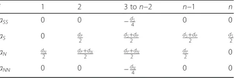
Applying boundary conditions on the continuity equa-tion requires a little care. The coefficients of Eq. (90) are presented in Tables1and2.

In order to apply the boundary conditions in the collo-cated grid, we go through the same way as for the stag-gered grid. It is noteworthy that in the collocated grid, more inner CVs are influenced by the boundary condi-tions than in staggered grid.

Vorticity calculation: we calculate vorticity at nodal points. According to Fig. 2, the vorticity for non-boundary nodes in the staggered grid is calculated by CDS:

ω¼∂_∂v x−

∂u ∂y¼

vI;j−vI−1;j

Δx −

ui;J−ui;J−1

Δy ð92Þ

In the collocated grid, velocity quantity on surfaces is calculated by averaging, and then vorticity is obtained by CDS approximation as follows:

ω¼∂v_∂x−∂u_∂y¼

vI;J−1þvI;J

2 −

vI−1;J−1þvI−1;J 2 Δx

−

uI−1;JþuI;J

2 −

uI−1;J−1þuI;J−1 2 Δx

ð93Þ

Results and discussions Staggered grid independency

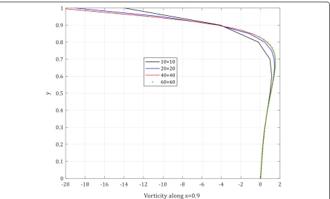
First, we need to examine the grid independence of the results. Grid independence study is carried out with FUDS, for Reynolds numbers of 10, 100, and 1000. The v-velocity profiles aty = 1/2 and the vorticity profiles at x =0.9 (due to the formation of the secondary vertex in the lower right corner of the area) are implemented to check grid independency, though the results of the latter are presented.

For Reynolds number of 10, the vorticity profiles at x = 0.9 are illustrated in Fig. 3. Four different grid systems of 10 × 10, 20 × 20, 40 × 40, and 60 × 60 are investigated. It is clear from the figure that the grid

independency is obtained by grid 40 × 40. Figure 4

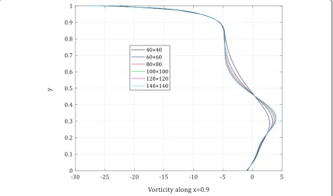
displays the vorticity profiles at x = 0.9 for grids 20 × 20, 40 × 40, 60 × 60, and 80 × 80 at Reynolds number of 100. Obviously, the grid independency for Re = 100 is obtained by grid 60 × 60. The vorticity profiles of grids 40 × 40, 60 × 60, 80 × 80, 100 × 100, 120 × 120, and 140 × 140 for Re = 1000 are presented in Fig. 5. The mesh independency in this case is obtained by grid 120 × 120.

Collocated grid independency

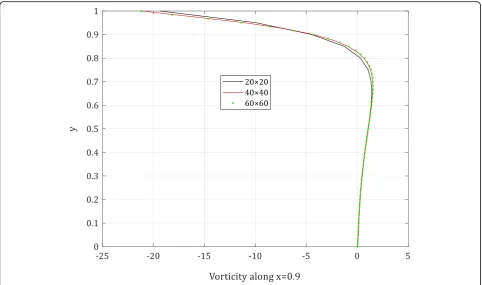
Similar to those done for the staggered grid, we use the vorticity profiles at x = 0.9 for investigating the grid in-dependence. The vorticity profiles at x = 0.9 and Reyn-olds number 10 is presented for grids 20 × 20, 40 × 40, and 60 × 60 in Fig.6. It is clear from the figure that grid independence is obtained by grid 40 × 40. Figure 7 pre-sents the vorticity profiles at x =0.9 and Reynolds num-ber 100 for grids 40 × 40, 60 × 60, and 80 × 80. This figure reveals that grid 60 × 60 is appropriate for inde-pendent results at Re = 100. The vorticity profiles at

x = 0.9 with Reynolds number 1000 are depicted for

grids 60 × 60, 80 × 80, 100 × 100, 120 × 120, and 140 × 140 in Fig. 8. It is clear from the figure that grid inde-pendency is obtained forRe =1000 by grid 120 × 120.

Consequently, collocated and staggered grids require the same grid size to attain independent results at each Reynolds number.

Table 1Coefficients of pressure correction equation which vary inx-direction

i 1 2 3 ton−2 n−1 n

aWW 0 0 −d₄W 0 0

aW 0 d₂P dW₂þdP dWþ₂dP d₂W

aE d₂E dPþ₂dE dPþ₂dE d₂P 0

aEE 0 0 −d₄E 0 0

Table 2Coefficients of pressure correction equation which vary iny-direction

j 1 2 3 ton−2 n−1 n

aSS 0 0 −dS

4 0 0

aS 0 dP

2

dSþdP 2

dSþdP 2

dS 2

aN dN

2

dPþdN 2

dPþdN 2

dP

2 0

aNN 0 0 −dN

Fig. 2Staggered grid arrangement

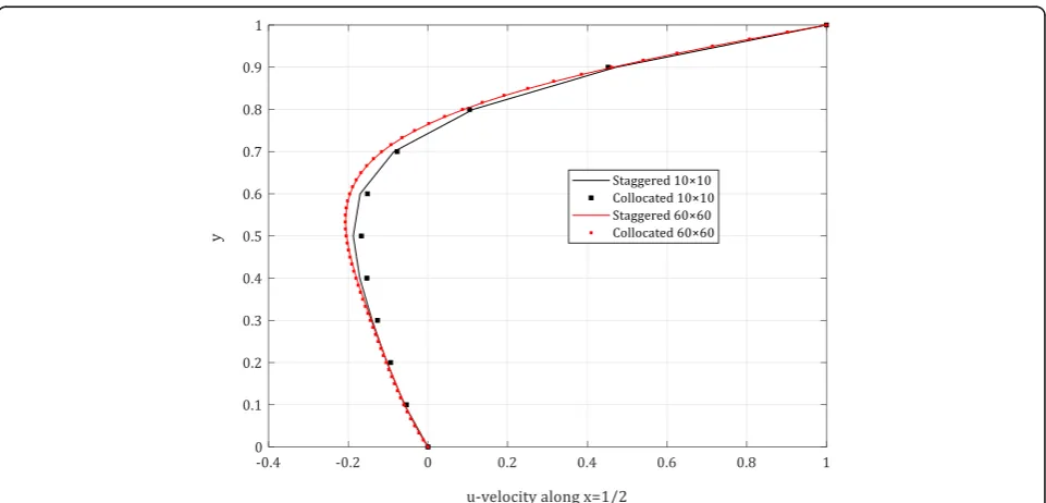
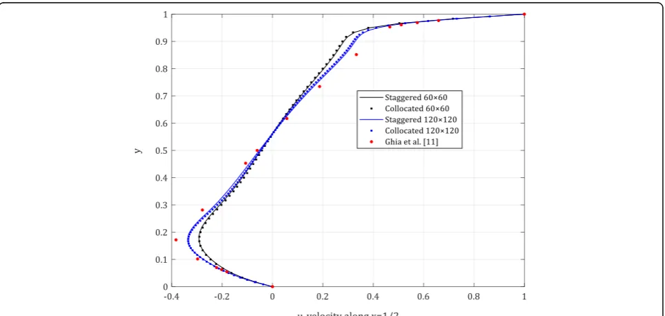
Staggered versus collocated

To compare the results of staggered and the collocated grids and compare them with benchmark of (Ghia, Ghia, and Shin,1982), Figs. 9,10, and11are provided. Theu -velocity profiles at x = 1/2 are shown for the three

Reynolds numbers of 10, 100, and 1000 obtained by FUDS. The results of (Ghia et al.1982) are presented as benchmark forRe =100, 1000.

The results prove that in cases of coarse grid (less number of nodes), the difference of the results of Fig. 4Staggered grid independency; vorticity profiles atx =0.9 forRe= 100

collocated grid and staggered grid is larger. Moreover, the values obtained with staggered grid are slightly more accurate than collocated ones by comparison with the reference values. It should be pointed out that the error of two implemented approaches is

higher in higher Reynolds numbers, especially in the regions with steep velocity gradients (see Fig. 11 for u at y= 0.17 and y= 0.85). This problem can be resolved by implementing a TVD scheme instead of the up-wind scheme.

Fig. 6Collocated grid independency; vorticity profiles atx =0.9 forRe= 10

FUDS versus SUDS

To compare the results of the second order UDS, with the results presented in the previous sections, which are obtained by the first order USD, simula-tions have been done with different number of nodes at Reynolds numbers 10, 100, and 1000. Prior to that, we studied the grid independency of the results

of SUDS. For Re = 10, grid 40 × 40 gives the

inde-pendent results identical to that of FUDS. At

Reynolds number 100, grid 50 × 50 and grid 40 × 40 give the independent results. However, with FUDS, the mesh independency is obtained by grid 60 × 60. Grid 80 × 80 attains independent outcomes, whereas the grid independence is obtained in grid 120 × 120 by FUDS.

According to the aforementioned results, it can be concluded that at low Reynolds numbers, the grid sizes in which independency is attained are the same Fig. 8Collocated grid independency; vorticity profiles atx =0.9 forRe= 1000

for both FUDS and SUDS. In contrast, at the high Reynolds numbers (Re > 100), FUDS require a finer grid than SUDS to attain independency. Consequently, the second order upwind scheme is an appropriate approximation for the large convection term at high Reynolds numbers.

Now, in order to compare the results of FUDS and SUDS, the u-velocity profiles at x = 1/2 are

illus-trated in Figs. 12, 13, and 14 respectively for 3

Reynolds numbers of 10, 100, and 1000 obtained with staggered grid. The results of (Ghia et al. 1982) are also brought in Figs. 13 and 14 for comparison.

With regard to these profiles, there is no superiority of SUDS over FUDS at low Reynolds numbers of 10. By contrast, SUDS has significantly less error than FUDS at Reynolds number 100 in coarse grids, and this issue reveals the SUDS accuracy in the approxi-mation of the momentum convection terms. Of Fig. 10u-velocity profilesat x =1/2 forRe= 100

course, the errors of both schemes reduce by fining the grid. In any case, SUDS have closer values to the reference results. The differences in values presented

in Fig. 14 for Re = 1000 are more obvious. In this

Reynolds number, FUDS has a considerable error even with a fine grid of 120 × 120 (noting that FUDS results are grid independent in this number of nodes). The SUDS results even by grid 40 × 40 have less error than grid independent results of FUDS. Furthermore,

SUDS with grid 120 × 120 exactly coincide with the benchmark of (Ghia et al. 1982).

Coupling algorithms of SIMPLE family

First, it must be noted that all previous results pre-sented in this report are obtained by SIMPLE

algo-rithm. To investigate the accuracy and the

performance of the algorithms in the iterative

solu-tion process, the residual of the x-momentum

Fig. 12FUDS versus SUDS;u-velocity profilesat x =1/2 forRe= 10

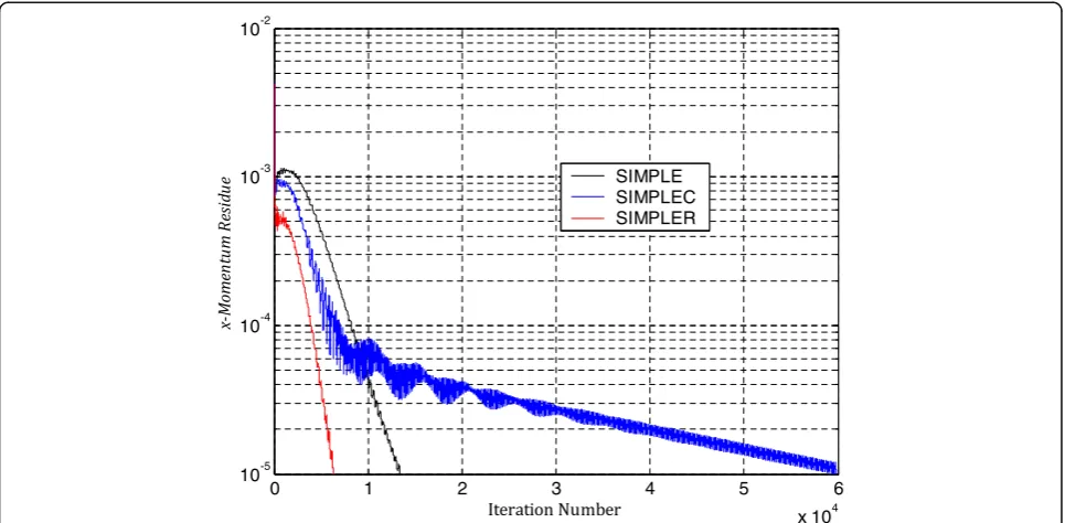
equation is plotted for 3 algorithms of SIMPLE family at Reynolds numbers of 10, 100, and 1000. The

re-sidual in terms of iteration number for Re= 10 for

SIMPLE, SIMPLEC, and SIMPLER is shown in Fig. 15.

Obviously, the SIMPLER algorithm apparently con-verges with the number of iterations about 40% of

that of SIMPLE. Considering the fact that the number of calculations in each iterate involved in SIMPLER is about 30% larger than that for SIMPLE (Versteeg and Malalasekera, 2007), the simulation time SIMPLER is about half of the SIMPLE. Unfortunately, SIMPLER gives devastating oscillatory solution. SIMPLEC ranks Fig. 14FUDS versus SUDS;u-velocity profilesat x =1/2 forRe= 1000

the second in speed but it causes oscillatory solution and of course less than SIMPLER.

Figure16depicts the residual of algorithms atRe =100. The performance of SIMPLE and SIMPLEC algorithms are alike and nearly smooth while SIMPLER is still faster but substantially oscillatory. The residuals for Reynolds number 1000 are illustrated in Fig. 17. Here, the trends

are thoroughly different from the previous graphs. From iteration number 800 onwards, SIMPLEC algorithm loses its performance and its convergence rate drops. SIMPLE and SIMPLER behave fairly smooth with ac-ceptable convergence rate. Multiplying the number of it-erations by the number of calculations in each iterate ranks SIMPLER as the fastest.

Fig. 16Performance of different coupling algorithms atRe= 100

Fig. 18Comparison of methods;u-velocity profile atx =1/2 forRe= 1000

All in all, SIMPLEC algorithm is a proper choice for low Reynolds numbers of order of 10, SIMPLE is suitable for Reynolds numbers of order of 102, and SIMPLER is the fastest for moderate Reynolds num-bers of order of 103.

Overall comparison of the methods

In order to sum up the results of FUDS versus SUDS, and staggered grid versus collocated grid, and also to compare with the reference, u-velocity profiles along y -axis x =1/2 andv-velocity profiles alongx-axis aty =1/

2 for Re = 1000 are depicted in Figs. 18 and 19,

respectively.

According to the two figures, it can be inferred that FUDS is rather inaccurate due to numerical diffusion es-pecially in the regions with large gradients, and it makes the velocity profile smoother. Moreover, staggered and collocated grids have the same results with FUDS. Nevertheless, with SUDS, staggered grid has more accur-acy than the collocated grid. It is remarkable that the re-sults of staggered grid with 120 × 120 and SUDS coincide with the results of (Ghia et al. 1982). Totally, staggered grid with SUDS gives the most accurate results followed by collocated grid with SUDS.

Conclusion

In the present paper, a lid-driven cavity problem is modeled via two basically different approaches of spatial discretization: collocated and staggered. From CFD point of view, it is noteworthy that the semi-discrete equations of the staggered grid and the collo-cated grid are similar. The main difference is in the calculation of convecting velocities and applying the boundary conditions.

Grid independency study proves that collocated and staggered grids require equal grid size to attain inde-pendent results at same Reynolds numbers. By coarse grid, the difference of the results of the collocated grid and the staggered grid is larger. Also, the error of two approaches is higher in higher Reynolds numbers, espe-cially in the regions with steep gradients. At low Reyn-olds numbers, the grid size in which independency is attained is the same for both FUDS and SUDS. In con-trast, at the moderate Reynolds numbers, FUDS require a finer grid than SUDS to attain independency. There is no superiority of SUDS over FUDS at low Reynolds numbers whereas SUDS has considerably less error than FUDS at moderate Reynolds numbers. By comparing dif-ferent coupling algorithms it can be concluded that SIMPLEC algorithm is a proper choice for low Reynolds numbers of order of 10, SIMPLE is suitable for Reynolds numbers of order of 102, and SIMPLER is the fastest for moderate Reynolds numbers of order of 103.

Briefly, FUDS is rather inaccurate due to numerical diffusion especially in the regions with large gradients, and it makes the velocity profile smoother and stag-gered, and collocated grids have the same results with FUDS. Besides, staggered grid with SUDS gives the most accurate results followed by collocated grid with SUDS.

Nomenclatures Across-sectional area

acoefficient in discretized equation bsource term

dpressure term coefficient Lcavity dimension Ppressure

P0reference pressure

ReReynolds number

uvelocity inx-direction u0lid velocity

vvelocity inx-direction xlongitudinal coordinate ytransversal coordinate

Greek letters ρdensity

μdynamic viscosity

Subscripts

Inode number inx-direction iface number inx-direction Jnode number iny-direction jface number iny-direction

Superscripts

*dimensional parameter

Acknowledgements

The authors express their special thanks to Professor Ali Ashrafizadeh from K.N. Toosi University of Technology for all his help.

Authors’contributions

AAB has developed the model and wrote the computer code. MMH has written the manuscript text and prepared the figures. The manuscript text is finally amended by AAB. Both authors read and approved the final manuscript.

Funding

This research does not have any funding.

Availability of data and materials

The output data of the computer code will be available on request via email to the corresponding author.

Competing interests

Received: 27 April 2019 Accepted: 20 June 2019

References

Ding, P. (2017). Solution of lid-driven cavity problems with an improved SIMPLE algorithm at high Reynolds numbers.International Journal of Heat and Mass Transfer, 115, 942–954.

dos Santos, D. D. O., et al. (2011). Numerical approximations for flow of viscoplastic fluids in a lid-driven cavity.Journal of Non-Newtonian Fluid Mechanics, 166(12_–13), 667_–679.

Elshehabey, H. M., & Ahmed, S. E. (2015). MHD mixed convection in a lid-driven cavity filled by a nanofluid with sinusoidal temperature distribution on the both vertical walls using Buongiorno’s nanofluid model.International Journal of Heat and Mass Transfer, 88, 181_–202.

Ghia, V., Ghia, K. N., & Shin, C. T. (1982). High-resolutions for incompressible flow using the Navier-stokes equations and a multi-grid method.Journal of Computational Physics, 48, 387–411.

Gutt, R., & Gro_şan, T. (2015). On the lid-driven problem in a porous cavity. A theoretical and numerical approach.Applied Mathematics and Computation, 266, 1070–1082.

Indukuri, J. V., & Maniyeri, R. (2018). Numerical simulation of oscillating lid driven square cavity.Alexandria Engineering Journal, 57, 2609_–2625.

McDonough, J. M. (2007). Parallel simulation of turbulent flow in a 3-D lid-driven cavity. InParallel computational fluid dynamics 2006(pp. 245–252). Elsevier Science BV.https://www.sciencedirect.com/science/article/pii/

B978044453035650033X.

Patil, D. V., Lakshmisha, K. N., & Rogg, B. (2006). Lattice Boltzmann simulation of lid-driven flow in deep cavities.Computers & Fluids, 35(10), 1116–1125. Peng, Y.-F., Shiau, Y.-H., & Hwang, R. R. (2003). Transition in a 2-D lid-driven cavity

flow.Computers & Fluids, 32(3), 337_–352.

Tamer, A. A. M., Khalid, M. S., Mohamed, A. K., & Ahmed, A. A. (2017). Revisiting the lid-driven cavity flow problem: Review and new steady state benchmarking results using GPU accelerated code.Alexandria Engineering Journal, 56, 123_–135.

Versteeg, H. K., & Malalasekera, W. (2007).An introduction to computational fluid dynamics: The finite volume method(2nd ed.). Pearson Education.https:// www.amazon.com/Introduction-Computational-Fluid-Dynamics-Finite/dp/ 0131274988. https://pearson.com.au/products/Versteeg-Malalasekra/An-Introduction-to-Computational-Fluid-Dynamics-The-Finite-Volume-Method/ 9780131274983?R=9780131274983.

Yapici, K., Karasozen, B., & Uludag, Y. (2009). Finite volume simulation of viscoelastic laminar flow in a lid-driven cavity.Journal of Non-Newtonian Fluid Mechanics, 164, 51–65.

Publisher’s Note