ORIGINAL ARTICLE
Simulating Tensile and Compressive
Failure Process of Concrete with a User-defined
Bonded-Particle Model
Jinhui Ren , Zhenghong Tian
*and Jingwu Bu
Abstract
A user-defined bonded-particle model (UBM) which is based on the modified parallel bond was established in this paper to investigate the tensile and compressive failure mechanism of concrete on the three-dimensional (3D) level. The contact constitutive relation and the failure criterion of the UBM can be added to the commercial discrete ele-ment software PFC3D by compiling them as a dynamic link library file and loading it into PFC3D whenever needed. In addition, the aggregate particles can be generated according to the volume fraction and the shape of each aggre-gate is irregular. Then, by comparing the results of numerical simulation with the results of laboratory tests, it is found that this bonded-particle model can simulate the tensile and compressive failure process of concrete well to a certain extent. Specifically, the two have basically similar failure patterns and stress–strain responses no matter under tension or compression loading condition. All results indicate that this UBM is a promising tool in understanding and predict-ing the tensile and compressive failure process of concrete.
Keywords: three-dimensional simulation, failure process, concrete, user-defined bonded-particle model, PFC3D
© The Author(s) 2018. This article is distributed under the terms of the Creative Commons Attribution 4.0 International License (http://creat iveco mmons .org/licen ses/by/4.0/), which permits unrestricted use, distribution, and reproduction in any medium, provided you give appropriate credit to the original author(s) and the source, provide a link to the Creative Commons license, and indicate if changes were made.
1 Background
Concrete has been widely used as an extremely impor-tant building material for more than one century. During this period, a large number of scholars have made lots of in-depth research on its mechanical properties and fail-ure mechanism. However, in most of the previous engi-neering application, people usually still treat concrete as a homogenous material and the macroscopic elas-tic–plastic theory is used to describle its whole process of deformation and failure in order to facilitate the study. Actually, the mechanical behaviors of concrete at macro-level are strongly affected by its mesoscopic structures (Nitka and Tejchman 2015), thus those simplifications of concrete are unreasonable from this perspective.
With the rapid development of the discrete element methods (DEM), a growing number of scholars come to use this approch in the field of granular materials (Baleviius et al. 2006; Kaianauskas et al. 2010; Latham
et al. 2013) and geotechnical engineering (Azevedo and Lemos 2013; Sarfarazi et al. 2014; Sarfarazi and Haeri
2016). The main advantage of DEM is the feasibility to model highly complex poly-dispersed systems by using the basic data on individual particles without making oversimplifying assumptions (Kaianauskas et al. 2010). So more and more researchers are striving to apply this approch to the simulation of concrete although some conventional methods, such as the finite difference, finite element and boundary element methods, can also simulate the concrete or concrete-like materials to some extent (You et al. 2012; Zhang et al. 2014; Shu-guang and Qingbin 2015; Haeri et al. 2013; Haeri 2015). However, there are a significant portion of concrete models built on the two-dimensional (2D) level (Cam-borde et al. 2000; Brara et al. 2001; Nagai 2004; Wang
2008; Azevedo 2008; Azevedo et al. 2010; Kim and Buttlar 2009; Kim et al. 2009; Lian et al. 2011a, b; Haeri and Sarfarazi 2016) which are considered to be difficult to accurately capture the interlock effect of particles in the 3D domain (Chen et al. 2011). In addition, material responses of the 3D simulation become more ductile
Open Access
*Correspondence: [email protected]
College of Water Conservancy and Hydropower Engineering, Hohai University, Nanjing 210098, China
compared with the results of 2D simulation and the stress fluctuations are relatively smaller due to a higher coordination number (Nitka and Tejchman 2015). Recently, 3D asphalt concrete simulation systems based on the Burger’s model (Chen et al. 2011; Liu et al. 2012) and 3D fresh concrete simulation systems based on the Bingham model (Shyshko and Mechtcherine 2013; Remond and Pizette 2014; Mechtcherine and Shyshko
2015) or the linear-spring dashpot model (Tan et al.
2015) have been gradually built up. But due to the lack of relatively appropriate constitutive models, the 3D simulation achievements for ordinary concrete are still very few. Hentz et al. (2004) developed a 3D discrete element model to study the dynamic behavior of con-crete at high strain rates and Nagai et al. (2005) also successfully put forward a 3D rigid body-spring model (RBSM) to predict the failure behavior of concrete. But it is a pity that the shape of the coarse aggregates in their models is spherical and that means the shape effects of aggregates are not discussed. Subsequently, Kozicki et al. described a quasi-static mechanism of fracture in concrete specimens under multiple loading conditions by using a 3D novel lattice model (Kozicki and Tejchman 2008; Kozicki and Donz 2008). Although the results are satisfactory, yet it is not found in their articles whether the model can also effectively simulate the concrete subject to compression. Recently, Nitka and Tejchman (2015) have attempted to reproduce the mechanical behaviors of concrete by using a 3D dis-crete element model YADE which was first developed in University of Grenoble. But for the sake of simplicity, the spheres were assumed to approximately simulate both the aggregates and mortar.
The intention of this paper is to present a 3D UBM of concrete which takes both the geometrical shapes and volume fraction of aggregates into consideration simul-taneously. It is worth mentioning that this new model is able to unify the two loading conditions, namely ten-sion and compresten-sion. In other words, it can simulate the mechanical behaviors of concrete well to a certain extent in two cases (tension and compression) by using the same UBM and the same set of model parameters. The rest of the paper is organized as follows: In Sect. 2, the 3D mathematical model of concrete specimen are presented in detail. Section 3 first explains the contact constitutive relation and the failure criterion of the UBM, then solves the problem how to assign the mesoscopic mechanical parameters to the model. Subsequently, a few contrast tests for numerical models and physical models are introduced in Sect. 4. Finally, the predicted results of the numerical simulation are compared with laboratory experimental measurements in Sect. 5, while the discus-sion and concluding remarks are given in Sect. 6.
2 3D Mathematical Model of Concrete Specimen 2.1 Generation and Replacement of Irregular Aggregate
Particles
As a kind of heterogeneous material, concrete is usually assumed to be a three-phase composite consisting of aggregates, mortar and the interfacial transition zones (ITZs) between them. Scanning electron and backscat-tered electron micrography evidenced the zones of defi-cient clinker concentration to be 15–30 μm (Lian et al.
2011b). Here we use the average value of this range (namely 23µ m) as the thickness of ITZs. Its
mechani-cal properties are influenced by the aggregate shapes to a certain extent. Piotrowska et al. (2014) pointed out the influence of coarse aggregate types on concrete behavior under high triaxial compression loading condition and Shigang et al. (2013) confirmed that the aggregate geo-metrical shapes has great effect on the failure behavior of the polyurethane polymer concrete (PPC) under tension. Rocco and Elices (2009) also explored the influence of aggregate shapes on the fracture energy, tensile strength and elastic modulus in concrete. What’s more, according to the research of Azevedo and Lemos (2006), it is shown that non-circular particles will lead to an increase in the post-peak ductility both in tension and in compression when the heterogeneous approach is adopted. Thus it is especially necessary to generate irregular aggregate par-ticles which can be regarded as polyhedrons if we want to simulate and predict the mechanical behaviors of con-crete more precisely.
On account of the difficulty existing in the discrete ele-ment calculation with polyhedrons, the most conveni-ent way of simulating polyhedrons is to bond the sphere particles into clumps. This idea can be achieved in PFC3D by executing the relevant commands of clump. There are two points worth highlighting:
• The polyhedrons in this paper are all convex polyhe-drons for the sake of simplicity.
• A clump itself will not break apart since it acts as a rigid body (with deformable boundaries).
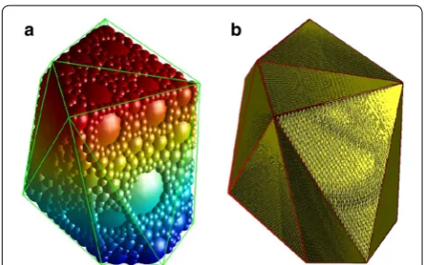
positions. We might as well call those sphere particles “loca-tors” and their role is to provide specific location informa-tion and necessary space for the replacement of clusters. It should be emphasized that the “locators” are randomly generated according to the transformed volume fraction of aggregates and their diameters are specified as uniform distribution in corresponding gradation ranges. Therefore, prior to the replacement of a cluster, we need to perform equal proportional scaling operation to guarantee that its paticle size is exactly equal to the diameter of the “locator” which remain to be replaced. Owing to the limited catego-ries and fixed angles of the particle clusters generated in MATLAB, it certainly doesn’t conform the stochastic char-acteristics of aggregate distribution if the rotation operation is not carried out. For this reason, an algorithm for rotation developed by Dong et al. is adopted in this study (Dong et al. 2007). In order to give consideration to both the preci-sion of aggregate shape and the efficiency of PFC3D solver simultaneously, the aggregate models used in numerical tests can’t be as elaborate as that in Fig. 1a. At the same time, in order to reflect the difference of aggregate shape, this paper uses four kinds of typical particle clusters before scaling, which correspond to four kinds of size intervals in aggregate gradation respectively. Figure 2 displays the A, B, C and D four kinds of typical particle clusters before scaling which are adopted in numerical models and their detailed shape parameters are shown in Table 1. Descriptions for some of those shape parameters (coefficient of irregularity, angularity and surface texture depth) can be found in the relevant literature (Barrett 1980; Hentschel and Neil 2003; Pourghahramani and Forssberg 2005).
2.2 Generation of Full‑Graded Concrete Cylinder Specimen Models
The diameter of concrete cylinder specimens is 72.0 mm and the height is about 156.0 mm. The reasons why its height is an approximate value are as follows:
• It is quite difficult to get an accurate model size since there is no universal method to limit the irregularly arranged compacted fillers in a specified sealed con-tainer and guarantee the upper surface is flat without execute moderate compression operation.
• The final height of numerical models is unable to be artificially determined because the height error need to be controlled within the allowable range by con-stantly fine-tuning the particle number of mortar phase.
In this paper, the final sizes of the models are
Φ72.0 mm×155.6 mm and Φ72.0 mm×155.4 mm
respectively for Group CA and Group CB. The two groups of concrete specimens have different mix propor-tions and the parameters of each component are shown in Table 2.
Obviously, according to Table 2, an aggregate can be represented by a clump only when its particle size is larger than 8.0 mm because the minimum particle size of the clump internal structure sphere is 1.8 mm (maxi-mum allowable overlap is 0.675 mm). If an aggregate is too small, the shape precision of its corresponding clump will be greatly reduced and the particle size will be inevi-tably lower than the actual value. As we know, the mortar is a mixture of sand and set cement. But here we treat it as one component for the consideration of computational efficiency. However, as you can see, we haven’t given the specific volume fraction of the mortar in Table 2 because it is impossible to be as dense as the real mortar. The deviation of the void ratio seems to be a serious problem that can not be ignored. But it is worth mentioning that the UBM is based on the MPB, the partial void between the particles can be considered to be filled with those Fig. 1 Cluster generated by MATLAB. a Cluster consists of 1348
paticles, b isoparametric grid map.
abstract parallel bonds which are able to transmit both forces and moments. In this way, as long as the parallel bond radius and other parameters are set reasonably, the influence of void ratio on the meso mechanical behaviors of concrete can be significantly decreased. The advantage is also the reason why the theory of parallel bond is often used to simulate some dense materials (Tan et al. 2015; Azevedo and Lemos 2013) and it has been confirmed that the parallel bonds are quite proper to model the hydrated cement paste around the aggregates (Lian et al.
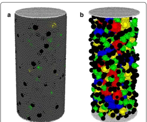
2011b; Azevedo 2008; Azevedo et al. 2010; Haeri and Sarfarazi 2016). The final model (just take Group CA for example) and its aggregate distribution map are shown in Fig. 3a, b respectively. Specifically, Fig. 3a shows a com-plete concrete cylinder specimen model , which contains aggregate particles, mortar particles (whose color is gray) and “ball-walls” (whose color is white). Figure 3b shows its corresponding internal aggregate distribution map, which only contains aggregate particles and “ball-walls”. The total paticle numbers of the final models are 39,208 and 38,994 respectively for Group CA and Group CB. The total contact numbers (excluding internal contacts of clumps) of the final models are about 3.8 times as much
as the corresponding paticle numbers, namely 150,659 and 147,020.
Table 1 Shape parameters of typical clusters before scaling.
Types of clusters Shape parameters
Size [size (length (mm) × width
(mm) × height (mm))] Number of internal structure spheres Coefficient of irregularity Angularity Surface texture depth (mm)
A 15.27×14.00×12.73 106 1.832 1.527 0.379
B 13.09×12.00×10.91 72 1.910 1.548 0.403
C 10.91×10.00×9.09 39 1.698 1.550 0.461
D 8.73×8.00×7.27 20 1.613 1.530 0.396
Fig. 3 The final model and its aggregate distribution map. a Final model, b aggregate distribution map.
Table 2 Parameters of each component.
Group Names of component Volume fraction(%) Minimum particle size
(mm) Maximum particle size (mm) Corresponding clump type
CA Aggregate component 1 7.058 14.00 16.00 A
Aggregate component 2 7.058 12.00 14.00 B
Aggregate component 3 7.058 10.00 12.00 C
Aggregate component 4 7.057 8.00 10.00 D
11.469 4.75 8.00
Mortar and voids 60.300 2.66 2.66
CB Aggregate component 1 7.353 14.00 16.00 A
Aggregate component 2 7.353 12.00 14.00 B
Aggregate component 3 7.353 10.00 12.00 C
Aggregate component 4 7.353 8.00 10.00 D
11.948 4.75 8.00
3 Assignment of the Mesoscopic Mechanical Parameters
3.1 Contact Constitutive Relation and Failure Criterion of the UBM
The overall mechanical behaviors of a material is simu-lated in PFC3D by associating the constitutive relation and failure criterion with each contact. The so-called constitutive relation consists of four parts:
• An relation between the contact force and relative linear displacement.
• An relation between the contact moment and relative angular displacement.
• An relation between normal and shear contact forces which permits the two contact balls to have a relative slip.
• Residual strength theory for bonds which belong to the non-ITZs.
The failure criterion serves to limit the maximum tensile, compressive and shear stresses of a contact. Alternate constitutive relation and failure criterion are also avail-able by loading the subprogram provided by user them-selves into PFC3D and this way is adopted in this paper for creating a new model.
As has been stated above, the UBM is based on the MPB which has a more complex failure criterion com-pared with the built-in parallel bond (BPB) (Minneapo-lis 2005). As we know, a BPB is defined by the following five parameters: normal and shear stiffnesses ( k¯n
i and k¯is [stress/displacement]); normal and shear strengths ( σ¯ and τ¯ [stress]); and bond radius R¯ . It will be broken when the normal or shear forces exceed their corresponding strengths. Obviously, the tensile strength is equal to the compressive strength by default and they are character-ized by using the same parameter σ¯ which can not unify the loading conditions of tension and compression cor-rectly. What’s more, the shear strength shouldn’t be a fixed value because it is affected by the normal force. The MPB, however, is defined by the following seven param-eters: normal and shear stiffnesses ( k¯n
i and k¯is [stress/dis-placement]); tensile and compressive strengths ( σ¯t and
¯
σc [stress]); cohesive force and interior friction angle (c
[stress] and ϕ [degree]) and bond radius R¯ which is desig-nated as the geometric mean of the two adjacent particle radii in this paper (see Eq. (1)). The reason why we don’t use the arithmetic mean is that it can’t well reflect the geometric relation for such a geometric quantity, bond radius.
Apart from having a more elaborate failure criterion, the MPB is also different from the BPB on the matter (1)
¯
R=R[A]·R[B]
whether it can coexist with the linear-stiffness model. As mentioned above, we treat mortar matrix as one com-ponent. However, it doesn’t agree with the homogeneity because the stiffness in the overlapping part between a BPB and its corresponding contact entities will be dou-ble counted, which will certainly lead to an unreasonadou-ble bigger overall stiffness composed of two parts (parallel-bond stiffness and linear contact stiffness). Instead, the existence of a MPB will preclude the possibility of the linear-stiffness model. As to the relation between nor-mal and shear contact forces, a slip model is defined in this paper and the slip condition will be judged by Eqs. (2) and (3). Moreover, the BPB and the behavior of rela-tive slip can occur simultaneously while the MPB will preclude the possibility of the slip model and the latter takes into consideration the quasi-brittle characteristic of mortar matrix which makes it much closer to the real situation.
where µ [dimensionless] is taken to be the static friction coefficient of the two contact entities; Fin and Fis denote the normal and shear components of contact force vec-tor, respectively; and Fmaxs is the maximum allowable shear contact force.
When the MPB breaks, the linear-stiffness theory which assumes that the stiffnesses of the two contact entities act in series is adopted in the UBM. The con-tact normal secant stiffness and shear tangent stiffness ( kin and kis [force/displacement]) is given by Eqs. (4) and (5).
where the superscripts [A] and [B] denote the two enti-ties in contact; kn and ks are the normal and shear stiff-nesses [force/displacement] for a entity.
The contact stiffnesses relate the contact forces and relative displacements in the normal and shear direc-tions via Eqs. (6) and (7).
(2)
Fmaxs =µ|Fin|, compressive state
(3)
|Fis|>Fmaxs , relative slip condition |Fis|Fmaxs , relative static condition
(4)
kin= k
[A] n kn[B]
kn[A]+kn[B]
(5) kis= k
[A] s ks[B] ks[A]+ks[B]
(6)
Fin=kinUnni
where Un [scalar] is the sphere overlap (positive; nega-tive, for a gap) in the normal direction and ni denote a
unit-normal vector on a contact plane. Us is the shear component of a contact displacement–increment vector which is used to calculate the shear force-increment vec-tor Fis.
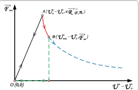
As you can see, the theory of elastic mechan-ics is employed to describe the behaviors of contact bonds before them break. If we don’t take the residual strengths into consideration, the macroscopic stress– strain responses obtained by simulation are bound to be more brittle than the laboratory measurements. In order to solve this problem, Gitman et al. (2008) adopted an elasticity-based gradient damage model which is able to consider the residual tensile strength on mesoscopic scale. Even though this model is fine, but there are too many empirical parameters need to be designated, namely length-scale parameter ℓ , residual stress parameter α˜ and slope of softening β˜ . Another model (called isotropic damage model) adopted by He et al. (2011) has a different definition for damage parameter ̟ . Compared with the former, their dam-age model just have two empirical parameters, namely the width of damage zone R and a parameter ℏ related to element size. However, the above two models are all based on the finite element method (FEM) and it is not easy to determine the values of those empirical param-eters in 3D discrete element models. Inspired by their damage models, we developed a simplified residual strength theory which is based on power function and only one empirical parameter is needed. With regard to this theory, the relation curve for strength and defor-mation is shown in Fig. 4. The red, green and blue lines in Fig. 4 represent the possible change paths of bond residual strength with deformation, while the black line stands for the elastic behavior before the corresponding bond cracks. Suppose the tensile deformation of a bond continues to increase to the state of arbitrary point B in Fig. 4, there would be two possible circumstances:
• Providing that the tensile deformation begins to decrease, the state point immediately changes into the path represented by the green line.
• Providing that the tensile deformation continues to increase, the state point gets into the path repre-sented by the blue line.
It is worth mentioning that this simplified residual strength theory will come into play only when the tensile failure occurs for a bond which belongs to the non-ITZs. The residual normal force F¯n
ires carried by the MPB is calculated through Eq. (8).
where U0n is the initial sphere overlap (positive; nega-tive, for a gap), Upn is the sphere overlap when the bond reaches its tensile strength σ¯t and Uminn is the minimum
sphere overlap which the bond has ever reached. The attenuation coefficient ð of residual strength will be an empirical constant (0.7 for models in this paper) if models are built under the same meso scale. Compared with the non-ITZs, the damage paths of ITZs are rela-tively fixed and the attenuation coefficient ð will be more greater. For simplicity, the residual strengths of ITZs have been ignored in this paper. In addition, the residual shear force F¯s
ires carried by the MPB is calculated through Eqs.
(9) and (10) when the tensile failure occurs for a bond which belongs to the non-ITZs.
where F¯s
i is shear force and F¯imn denotes the correspond-ing normal force of minimum sphere overlap Uminn .
Like-wise, k¯n
im denotes its corresponding normal stiffnesses which will be used in the calculation of bending moment.
(8)
¯ Firesn =
0, Uminn Un<U0n πR¯2σ¯tni(U
n−Un
0 Un
p−U0n)
−ð
, Un<Uminn
(9)
¯
Firess =℘F¯is
(10)
℘=
1, if| ¯Fis| τ¯| ¯F
n im|
¯
σt
¯
τ| ¯Fimn|
¯
σt| ¯Fs i|
, if| ¯Fis|> τ¯| ¯F n im|
¯
σt
(11) ¯
kimn = | ¯F n im|
πR¯2(Un
0 −Uminn )
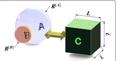
3.2 Relation Between Macro‑ and Meso‑Properties The material macroscopic responses can be deter-mined by their corresponding set of deformability and strength parameters of the mesoscopic structures. The behavior of a contact between two particles can be considered as an elastic square-section beam with its ends at the particle centers and this idea is illustrated in Fig. 5. The length L as well as the cross-sectional length
˜
L of the beam can be expressed as the average of the two particle diameters, then the cross-sectional area of the beam is given by Eq. (13):
The two particles will have the same normal and shear stiffnesses ( kn and ks ) if they belong to the same material and their radii are equal. Then the contact nor-mal and shear stiffnesses are found, using Eqs. (14) and (15), to be:
For pure normal and pure shear loading, the normal and shear behaviors are uncoupled and that means the kin and kis also can be expressed as the following equations if the Young’s modulus E and the Poisson’s ratio ν of the material are known to us. The derivation process of the two formulas are similar to Azevedo’s relevant literature (Azevedo 2008; Azevedo et al. 2010).
(12)
L= ˜L=R[A]+R[B]
(13) A= ˜L2
(14) kin= kn
2
(15)
kis= ks 2
(16)
kin= EA L
Two expressions for kn and ks can be obtained by substi-tuting Eqs. (12), (13), (14) and (15) into Eqs. (16) and (17), then rearranging them:
where R is the radius of the sphere whose stiffness parameters remain to be assigned.
The behavior of the MPB in this paper is similar to an elastic circular-section beam whose length, L¯ in Fig. 6, approaches zero. Relative motion causes normal and shear forces ( F¯n
i and F¯is , respectively) as well as bend-ing and torsional moment ( M¯n
i and M¯is , respectively) to develope. Before the MPB is destroyed, we use a circu-lar-section beam model. Once the MPB is damaged, a rectangular beam model (see Fig. 5) will be activated.
As we know, the concrete is generally considered to be a three-phase composite composed of aggregates, mortar and the ITZs between them. However, as the weakest link in the concrete, it has been recognized that the ITZs (aggregate–aggregate, aggregate–mortar) play a crucial role in the macro-properties of the con-crete due to its higher porosity, lower Young’s modulus and lower tensile strength compared with the mortar (Shuguang and Qingbin 2015).
For pure normal and pure shear loading, the normal and shear behaviors are uncoupled and the normal and shear stiffnesses of the MPB ( k¯n
i and k¯is , respectively) can be expressed as the following equations:
(17)
kis= EA
2(1+ν)·L
(18) kn=4ER
(19) ks=
2ER 1+ν
(20)
¯ kin= k
n i A =
E
L, for the mortar-mortar ξ·E
L , for the ITZs Fig. 5 Contact behavior depicted as a square-section beam.
where ξ denotes the reduction factor of the Young’s modulus for the ITZs and its value can be taken as 0.45 according to the present research achievements (Yang
1998).
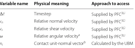
The calculation cycle in PFC3D is a timestepping algo-rithm that requires the repeated application of the law of motion to each particle, a force-displacement law to each contact and a constant updating of wall posi-tions (Minneapolis 2005). This algorithm can recognize the movement and interaction of particles precisely for any time interval (Lian et al. 2011a) and this process is illustrated in Fig. 7. In the software PFC3D, it is worth mentioning that the timestep adjustment is automatic and it is no need to worry about problems such as par-ticle penetration, result distortion and numerical insta-bility caused by those large timesteps. It is one of the main advantages of this software that it can automati-cally adjust timestep and ensure the convergence of the calculation results. There are several variables, listed in Table 3, need to be accessed by the MPB dynamically which are used to compute the mechanical responses of the UBM during cycling.
Then the normal and shear forces ( F¯n
i and F¯is , respec-tively) carried by the MPB can be written as:
(21) ¯
kis= k s i
A =
E
2(1+ν)·L, for the mortar-mortar
ξ·E
2(1+ν)·L, for the ITZs
(22) F¯in=vntk¯inA¯
(23) F¯is=vstk¯isA¯
where F¯in and F¯is are the normal and shear force-increment vectors of the UBM respectively; The cross-sectional area of the MPB A¯ is given by Eq. (26); The moment and polar moment of inertia ( I¯ and ¯J , respec-tively) are given by Eqs. (27) and (28):
(24)
¯
Fin= −F¯in
(25) ¯
Fis= −F¯is
(26) ¯
A=πR¯2= 14π (R[A]+R[B])2
(27)
¯
I = 14πR¯4= 641 π (R[A]+R[B])4
(28) ¯
J=2I¯
Fig. 7 Calculation cycle in PFC3D .
Table 3 MPB variables accessed dynamically during cycling.
a The relative angular velocity supplied by PFC3D adopts degree measure. A
conversioncoefficient α is designated here for translating the degree into radian and it can be expressedas α = π/180.
b Note that the contact unit-normal vector isn’t supplied by PFC3D directly, so
the au-thors developed a program to calculate it every certain and appropriate timesteps since thedeformation of the UBM is quite slowly.
Variable name Physical meaning Approach to access
t Timestep Supplied by PFC3D
vn Relative normal velocity Supplied by PFC3D
vs Relative shear velocity Supplied by PFC3D
ω Relative angular velocitya Supplied by PFC3D
Then the bending and torsional moment-increment vec-tors ( M¯ni and M¯si , respectively) carried by the MPB can be written as:
where ζn and ζs denote the normal and shear component vectors of the relative angular velocity [radian meas-ure]; The total moment associated with the MPB can be expressed as M¯i via:
Local non-viscous damping, to dissipate the excessive kinetic energy by effectively damping the equations of motion, is available in PFC3D . Fd
(i) is the damping force:
where F(i) is the resultant force (the sum of all externally applied forces acting on the particle) and it is controlled by the damping constant γ whose value can be chosen as 0.08 (Nitka and Tejchman 2015). Moreover, sign(•) denotes the sign function and V(i) is the generalized velocity given by Eq. (35).
where x(1)˙ , x(˙2) and x˙(3) are the translational velocities referred to the principal axes and ψ(1) , ψ(2) and ψ(3) are the angular velocities about the principal axes.
Frankly, the damping constant γ whose value is gen-erally taken as 0.08 (Kozicki et al. 2012, 2014; Nitka and Tejchman 2015) has a little influence on the stress–strain responses in our paper no matter under tension or com-pression loading condition. According to our research, the peak stress deviations ( <1 MPa for compression; <0.1 MPa for tension) are almost negligible. Because the loading speed in our article is much smaller than the loading speed in literature (Kozicki et al. 2012, 2014; Nitka and Tejchman 2015) especially for the tensile load-ing, there is little excess kinetic energy needed to be dis-sipated so that the effect of local nonviscous damping is not very significant. And this phenomenon has also been emphasized in the literature (Kozicki et al. 2014). The tensile, compressive and shear strengths of the MPB ( σ¯t ,
¯
σc and τ¯ , respectively) have a one-to-one correspondence
(29) ζn=(αω·ni)·ni
(30) ζs=αω−ζn
(31) �M¯in=ζs�tk¯in¯I
(32) �M¯is=ζn�tk¯is¯J
(33)
¯ Mi= −
(�M¯in+�M¯is)
(34) F(di)= −γ · |F(i)| ·sign(V(i)), i=1· · ·6
(35)
V(i)=
˙
x(i), for i=1· · ·3 ψ(i−3), for i=4· · ·6
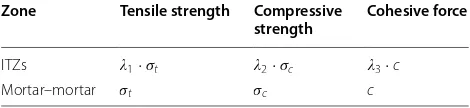
with the material strengths ( σt , σc and τ , respectively) since they are specified in stress units (see Table 4 for details).
where denotes the reduction factor of the strength for the ITZs and the value of 1 can be specified as 0.45 according to the current research results (Hongyi 2015; Azevedo 2008; Gu et al. 2013; Nagai et al. 2005). The aver-age value of 1 in these literature are basically within the range [0.4, 0.5]. Considering the effect of water cement ratio and joint roughness coefficient (JRC), we finally specified it as 0.45 by querying the provided experience curve in the dissertation (Hongyi 2015). Assuming that the ratio of the tensile strength, compressive strength and cohesive force remains unchanged, the values of 2 and 3 should be the same as that of 1 . Besides, the coefficient of strength variation ℵs and the coefficient of modulus variation ℵe also have been introduced into our models and their values are all 3%.
Unlike the BPB, the shear strength of a MPB isn’t a fixed value and Mohr–Coulomb criterion is chosen to calculate its shear strength dynamically as shown in Eq. (36).
The cohesive force c can be measured by direct shear test and the typical value of interior friction angle ϕ can be taken as 35◦ according to the relevant literature (Xianglin Gu et al. 2013).
4 Tests of Numerical Model and Physical Model 4.1 Tests of Numerical Model
4.1.1 Acquisition of Macroscopic Parameters
The mortar component in the concrete specimen con-sists of ordinary portland cement, water and sand (fine-ness modulus fluctuates between 2.3 and 3.0). The corresponding mass ratios of them are 1 : 0.68 : 2.59 and 1 : 0.49 : 1.50 respectively for Group MA and Group MB. The macroscopic tensile, compressive strengths and cohesive force are able to be obtained through the tensile test, compressive test and direct shear test respectively. Specifically speaking, the testing methods and facili-ties for the tensile and compression tests of the mortar specimens are similar to those used in the correspond-ing concrete tests. The size of the mortar specimens is 40 mm×40 mm×40 mm ( length×width×height )
(36)
¯
τ =c+ ¯σtanϕ
Table 4 Mesoscopic strength parameters of the MPB.
Zone Tensile strength Compressive
strength Cohesive force
ITZs 1·σt 2·σc 3·c
for compression and 40 mm×40 mm×160 mm ( length×width×height ) for tension. The reason why we measured the macroscopic tensile strength by uniaxial tensile test is that uniaxial tensile strength is more relia-ble than other tensile strengths (Haeri et al. 2016; Sarfar-azi and Schubert Sarfarazi and Schubert). With regard to the direct shear test of mortar specimens, the traditional rectangular short-beam direct shear test is adopted. As we know, the traditional rectangular short-beam direct shear test is the most commonly used method of direct shear test owing to its simple and intuitive design, which was first put forward and adopted by a German scholar Mörsch. During the test, both ends of a specimen were supported by two rigid plates. Then the mid-span load is applied to the rectangular short-beam through the upper rigid plate until it is destroyed and the size of the mortar specimens is 120 mm×40 mm×40 mm ( length×width×height ). The experimental results are as follows: Group MA: σt=3.02 MPa, σc=31.3 MPa and c=9.73 MPa; Group MB: σt=4.17 MPa, σc=52.2 MPa and c=16.7 MPa. Notice that Group MA and Group MB are the corresponding mortar phase specimens of Group CA and Group CB respectively.
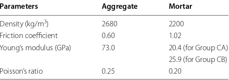
The aggregates in the concrete specimen are all crushed basalt whose joint roughness coefficient (JRC) is about 7.0. The approximate density value of the basalt and the mortar ( ρa and ρm , respectively) can be measured by the Archimedes method. Other parameters such as fric-tion coefficient µ , Young’s modulus E (The HS-bounds method (Simeonov and Ahmad 1995) is taken here and the average value of HS-bounds is used to estimate the Young’s modulus of the mortar phase) and Poisson’s ratio ν can be gained by consulting relevant literature (Franz et al. 2003; Richard 1993; Simeonov and Ahmad 1995; Schultz 1995) and their specific values adopted in this paper are listed in Table 5.
4.1.2 Loading Mechanism
PFC3D only allows particles to be bonded together at contacts, a particle may not be bonded to a wall. That is to say, it’s necessary to use the “ball-walls” composed of some sphere particles whose radii are 0.9 (maximum
allowable overlap is 0.45 mm) to simulate the condition of tension and the “ball-walls” are defined as clumps.
During the loading process, the strain of a specimen is captured by monitoring the Z coordinate variations of the contacts existing in the loading boundaries. It is assumed that the stiffness of the “ball-walls” is far greater than that of the specimens for the purpose of reducing the post-peak springback of the “ball-walls” and facilitat-ing the post-peak speed control of loadfacilitat-ing.
For the condition of tension, each contact between the “ball-walls” and the surfaces (top and bottom) of speci-mens is assigned with a MPB whose strength and stiff-ness are all far greater than those within the specimens in order to guarantee that it won’t crack and the post-peak springback of a MPB can be ignored so that the post-peak loading speed can’t be seriously affected by the rebound velocity of the MPB. The loading mode is uniaxial sym-metrical tension.
By contrast, there are no bond exist in the interfaces between the “ball-walls” and the surfaces (top and bot-tom) of specimens in the condition of compression. The friction coefficient of the “ball-walls” µw is consistent with that of the real loading plates, namely µw=0.15 . The loading mode is uniaxial symmetrical compression.
It is necessary to control the reasonable loading speed to ensure a quasi-static equilibrium (for discrete mod-els, literature (Haeri and Sarfarazi 2016; Sarfarazi et al.
2014; Ghazvinian 2012) suggest that 0.016m / s will be an appropriate loading speed while literature (Kozicki et al.
2014, 2012) suggest that 0.010 m/s will be an appropri-ate loading speed). The large-scale computing device provided by the Research Institute of Hydraulic Struc-ture (Hohai University) allows us to further reduce the loading speed to 0.00025 m/s for uniaxial symmetrical tension and 0.0025 m/s for uniaxial symmetrical com-pression. Therefore the loading speed is slow enough to ensure the tests are conducted under quasi-static condi-tions. Roughly speaking, the corresponding simulation times for tension and compression tests in our paper are all about 10 days (parallel-processing mode is off).
4.2 Tests of Physical Model
After those two groups of concrete specimens (Group CA and Group CB) were manufactured and formed, they were instantly placed in a suitable environment ( 20±5◦C ) and kept for 1 day, then they were moved to the standard curing room ( 20±2◦C for temperature and 95% for relative humidity) and kept for 28 days.
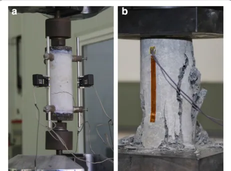
Each group of concrete specimens was planned to be used for two kinds of experiments, namely uniaxial ten-sile and compressive tests. MTS material testing system (as shown in Fig. 8a) and WAW microcomputer control electro-hydraulic servo testing machine (as shown in
Table 5 Relevant macroscopic mechanic parameters.
Parameters Aggregate Mortar
Density (kg/m3) 2680 2200
Friction coefficient 0.60 1.02
Young’s modulus (GPa) 73.0 20.4 (for Group CA) 25.9 (for Group CB)
Fig. 8b) are available for the uniaxial tensile and compres-sive tests respectively. Three extensometers are used for every tensile specimen to measure the axial tensile strain, while two strain gages are symmetrically arranged in the cylindrical surface of every compressive specimen to measure the axial compressive strain.
A kind of epoxy resin structural adhesive (bond tensile strength is about 10 MPa) is applied to cohere the load-ing plates ( Φ72 mm×20 mm ) and the ends of speci-mens before the uniaxial tensile tests. The pull rods fixed on loading plates should be connected with the fixtures of the MTS material testing system. It’s also essential to adjust the tightness degree of connecting bolts in the pull rods and align the pull rods and the central axis of a spec-imen as accurately as possible.
5 Comparison of Numerical and Experimental Results
5.1 Failure Patterns Under Different Loading Conditions The typical failure patterns of the laboratory tests under tensile and compressive loading conditions are shown in
Fig. 9a, b) respectively. Obviously, the typical failure pat-tern of concrete specimen in laboratory uniaxial tensile test is that the specimen has been divided into two parts Fig. 8 Testing devices. a MTS material testing system, b WAW testing machine.
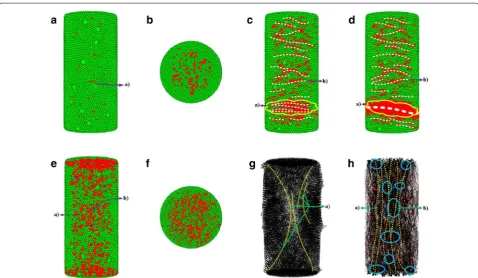
and its only main failure face is approximately parallel to the loading boundaries. In contrast, the typical fail-ure pattern of concrete specimen in laboratory uniaxial compressive test is that there are several main fault zones have been formed and almost all of them are approxi-mately perpendicular to the loading boundaries. As a comparison, the failure patterns of the numerical simula-tion can be illustrated and characterized mainly by two ways, namely crack tracking method and displacement nephogram method, respectively. Furthermore, two addi-tional ways, displacement vector diagram method and force chains diagram method, are necessary to be com-bined used in order to reflect the failure process of con-crete more comprehensively.
Just take Group CA for example, for the former main approach (crack tracking method), the damage formation thoughout the tensile specimen can be seen in Fig. 10a through Fig. 10d, which depict the cracking mode such as the orientation, location and type (red and blue cor-respond to normal failure and shear failure, respectively) of each microcrack at different deformation stages.
During the tensile loading process, microcracks initiated randomly, then formed several failure faces perpendicu-lar to the loading direction. With the increase of tensile deformation, some failure faces became the main failure face and eventually led to complete fracture of the tensile specimen.
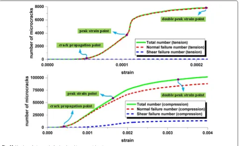
and shear failure numbers versus axial strain. It should be noted that the meaning of crack propagation point in this paper is the relatively obvious inflection point which connects the slow and rapid increase stages of the total number of microcracks rather than the state when the first microcrack appears (crack initiation defined in mesoscopic level). Obviously, for mesoscopic level, crack propagation has more practical significance compared with crack initiation. We can see it clearly that the total number of microcracks has a tendency of exponential growth after crack propagation point and finally tended to be gentle after peak strain point.
For the latter main approach (displacement nepho-gram method), the damage formation thoughout the specimens can be seen in Fig. 12a through Fig. 12h, which depict the axial displacement nephograms for tension and radial displacement nephograms for com-pression at different deformation stages. Obviously, the main failure faces of tensile numerical models and the main fault zones of compressive numerical models are all similar to the failure patterns of the laboratory tests (as shown in Fig. 9). Specifically speaking, Fig. 12a, b as well as Fig. 12e, f reflect the changes of failure faces under tensile loading condition and the main failure faces which present between the red and blue color
regions tend to be parallel with the loading bounda-ries. It is noteworthy that the main failure faces rapidly developed while the others almost had no changes after reaching the peak stress. Fig. 12c, d as well as Fig. 12g, h reflect the changes of fault zones under compres-sive loading condition and the main fault zones which roughly present between the yellow and cyan color regions tend to be oriented at a approximate angle range [0◦, 45◦] to the direction of loading application. In
addition, the phenomenon that some longitudinal main fault zones finally reached the loading boundaries is predicted.
5.2 Stress–Strain Responses Under Different Loading Conditions
The predicted stress–strain responses and their com-parison with experimental results under tensile and compressive loading conditions are shown in Fig. 13a, b respectively. It is worth mentioning that two complete stress–strain empirical curves (namely the dark green and light green dotted lines in Fig. 13b) under com-pression drew by a recommended empirical formula (Yiqiang et al. 2005) are used for reflecting the general trend of experimental curves whose downward sections
are hard to be obtained under the existing experimen-tal conditions. The recommended empirical formula about the stress σ˘c and strain ε under compression is as follows:
Where χ is the coefficient equal to the ratio of ini-tial elastic modulus E0 to peak secant modulus Ep and the value of it can be taken as 2.0 while the independ-ent parameter β can be taken as 0.8 and 2.0 respectively for Group CA and Group CB according to the literature (Zhenhai 1997). According to the experimental results, the values of axial compressive strength fp and the
(37)
˘
σc=
fp·
χ·ε εp−
ε2 ε2p 1+(χ−2)·εε
p
, (0ε < εp)
fp·
ε εp
β·(εε
p−1)
2+ε εp
, (εεp)
peak strain εp can be taken as follows: 24.54 MPa and
1.54×10⁻³ respectively for Group CA; 37.44 MPa and 1.88×10⁻³ respectively for Group CB.
For Group CA, we can find of the simulated and experimental curves have basically similar tendencies and strengths no matter under tension or compres-sion loading condition apart from the smaller peak strain (corresponding to the peak stress) of simulated stress–strain curve. As mentioned above, the residual strength of shear failure for a bond which belongs to the non-ITZs has been ignored, which will inevitably lead to the higher efficiency of energy accumulation for those unbroken bonds in numerical models. Maybe this is the main reason why the peak strain of simu-lated stress–strain curve is less than the experimental one especially for the compression loading condition. For Group CB, another major difference between the simulated and experimental curves embodies in the slopes of downward sections (also known as softening
branches) both for tension and compression. That the unloading rebound of a bond which is in the state of residual strength has been ignored might be the main reason why the downward slopes of numerical curves are flatter than those of the experimental ones.
What the simulated curves imply is that the stress σ˘ increased approximately linearly at first (the stage before crack propagation point), then a long distinctly nonlinear phase appeared when the crack propagation stress σ˘pro was reached (the stage between crack propagation point and peak strain point). Afterwards, the curves gradu-ally descented after they got to the peak stress σ˘max (the stage after peak strain point). As is known to us all, the definition of crack initiation point in macroscopic level is the point where the stress–strain curve begins to be nonlinear. With regard to the experimental curves, the crack initiation (defined in macroscopic level) stress can be roughly taken as 65% of the peak stress for the tensile condition (Feng 2006) while the corresponding stress index can be roughly taken as 40% of the peak stress for
the compressive condition (Zhenhai 1997) (mark points of the experimental curves have been omitted in the graphs). The comparison of relevant stress indexes for those mark points are listed in Table 6.
Strikingly, from the above comparison, the values of crack initiation (defined in macroscopic level) stresses are pretty close to those of crack propagation stresses. In particular, the ratio of crack propagation stress to peak stress are around 0.62 and 0.41% respectively for tension and compression which means the similarity of crack ini-tiation (defined in macroscopic level) stresses and crack propagation stresses is quite high. What’s more, the abso-lute values of peak stress relative errors are all below 7.0% which is within the allowable range. In brief, except for the relevant indexes about the residual stress corre-sponding to the double peak strain, other characteristic stress values of simulated mark points are all close to the experimental corresponding values no matter under ten-sion or compresten-sion loading condition.
6 Discussion and Conclusions
Some meso-level analyses of concrete are carried out by a 3D UBM in this study, which is able to take into account both the geometrical shapes and volume frac-tion of aggregates simultaneously. What’s more, the pro-posed method can simulate the mechanical behaviors of concrete well to a certain extent no matter under ten-sion or compresten-sion loading condition by using the same UBM and the same set of model parameters. Overall, the results of numerical simulation and laboratory tests have basically similar failure patterns and stress–strain responses. The discussion and concluding remarks drawn from this study are listed below:
• In the simulation of uniaxial tensile tests, several failure faces approximately parallel to the loading boundaries were formed (see Fig. 10c) and some of them would become the main failure faces which eventually divided the specimen into two parts (see Fig. 10d). After reaching the peak stress, the main failure faces rapidly developed while the others almost had no changes which can be called disturbed zones (see Fig. 12a, b as well as Fig. 12e, f).
• In the simulation of uniaxial compressive tests, sev-eral fault zones approximately perpendicular to the loading boundaries were formed and some of them would become the main fault zones which eventually ran through the specimen (see Fig. 10g, h as well as Fig. 12d, h).
• The total number of microcracks (broken bonds) in a specimen has a tendency of exponential growth after crack propagation point and finally tended to be gen-tle after peak strain point no matter under tension or Fig. 13 Stress–strain responses under mutiple loading conditions.
compression loading condition (see Fig. 11). Moreo-ver, the curves of corresponding normal and shear failure numbers show that the main failure mode of contact bonds is normal failure no matter under ten-sion or compresten-sion loading condition.
• By observing the colors and shapes of the incipient microcracks (see Fig. 10a, e), the authors find there are only red microcracks in the tensile specimen and most of them are transverse fusiform while there are both red and blue microcracks in the compressive specimen and most of them are longitudinal fusi-form. This phenomenon indicate that the incipient microcracks are mainly brought about by the normal forces and it can be inferred that their failure modes are tearing-tensile failure and bulging-tensile failure respectively.
• Since the simplified residual strength theory used in our models only applies to the situation when the tensile failure occurs for a bond which belongs to the non-ITZs, the residual strength of shear failure for a bond which belongs to the non-ITZs has been ignored. Consequently, with the increase of the shear failure number in numerical models, the efficiency of energy accumulation for those unbroken bonds in numerical models will be much higher than those in real specimens. Maybe this is the main reason why the peak strain (strain cor-responding to the peak stress) of the simulated stress–strain curve is less than the experimental one especially for compression loading condition.
• For the simplified residual strength theory adopted in this paper, the unloading rebound of a bond
which is in the state of residual strength has been ignored, which might be the main reason why the downward slopes of numerical curves are flatter than those of the experimental ones especially for Group CB. Specifically, the higher the strengths are, the relatively flatter the downward slopes of numerical curves will be. Of course, the precondi-tion is that the attenuaprecondi-tion coefficient ð of residual
strength remains unchanged.
However, the research findings and conclusions in this paper were only based on the two loading conditions, namely tension and compression. Deeper research will be performed in the future for the simulation of more loading conditions such as direct shear test and three-point bending test by using the 3D UBM. Additionally, the feasibility study of the simulation for concrete under combined loading conditions are also ongoing for further validation.
Authors’ contributions
JR carried out the experiment, the DEM simulation and drafted the manu-script. ZT superivised the whole study and gave guidances of the study. JB helped with the experiment and the data analysis. All authors read and approved the final manuscript.
Acknowledgements
This study is financially supported by national natural science fund of China (No. 51279054) and the Priority Academic Program Development of Jiangsu Higher Education Institutions in China (No. YS11001). In addition, fruitful discussions about the experiment schemes with Dr. Xudong Chen from Hohai University are acknowledged. Finally, The authors greatly appreciate the necessary support of testing facilities and the large-scale computing device provided by the Research Institute of Hydraulic Structure (Hohai University), Jinling Institute of Technology and the Nanjing Hydraulic Research Institute (NHRI).
Table 6 Comparison of relevant stress indexes for mark points.
* The value of residual stress corresponding to double peak strain is taken from empiricalcurve.
Group Stress indexes Uniaxial tensile tests Uniaxial compressive tests
Simulation Experiment Relative error (%) Simulation Experiment Relative error (%)
CA σini˘ 1.38 MPa 2.9 9.82 MPa 0.3
˘
σpro 1.42 MPa 9.85 MPa
˘
σmax 2.22 MPa 2.13 MPa 4.2 22.85 MPa 24.54 MPa −6.9
˘
σres 0.84 MPa 0.93 MPa −9.7 14.66 MPa 17.13MPa∗ −14.4
˘
σini/σ˘max 0.65 −1.5 0.40 7.5
˘
σpro/σmax˘ 0.64 0.43
˘
σres/σmax˘ 0.38 0.44 −13.6 0.64 0.70 −8.6
CB σini˘ 1.90 MPa −3.2 14.98 MPa −7.2
˘
σpro 1.84 MPa 13.90 MPa
˘
σmax 3.06 MPa 2.92 MPa 4.8 36.01 MPa 37.44 MPa −3.8
˘
σres 1.31 MPa 0.97 MPa 35.1 21.82 MPa 18.88 MPa 15.6
˘
σini/˘σmax 0.65 −7.7 0.40 −2.5
˘
σpro/˘σmax 0.60 0.39
˘
Competing interests
The authors declare that they have no competing interests.
Publisher’s Note
Springer Nature remains neutral with regard to jurisdictional claims in pub-lished maps and institutional affiliations.
Received: 13 May 2017 Accepted: 26 June 2018
References
Azevedo, N. M., & Lemos, J. V. (2006). Aggregate shape influence on the frac-ture behaviour of concrete. Structural Engineering and Mechanics, 24(4), 411–427.
Azevedo, N. M., Lemos, J. V., & de Almeida, J. R. (2008). Influence of aggregate deformation and contact behaviour on discrete particle modelling of fracture of concrete. Engineering Fracture Mechanics, 75(6), 1569–1586. Azevedo, N. M., Lemos, J. V., & Almeida, J. R. (2010). A discrete particle model
for reinforced concrete fracture analysis. Structural Engineering and Mechanics, 36, 343–361.
Baleviius, R., Diugys, A., Kaianauskas, R., Maknickas, A., & Vislaviius, K. (2006). Investigation of performance of programming approaches and lan-guages used for numerical simulation of granular material by the discrete element method. Computer Physics Communications, 175(6), 404–415. Barrett, P. J. (1980). The shape of rock particles, a critical review. Sedimentology,
27(3), 291–303.
Brara, A., Camborde, F., Klepaczko, J. R., & Mariotti, C. (2001). Experimental and numerical study of concrete at high strain rates in tension. Mechanics of Materials, 33(1), 33–45.
Camborde, F., Mariotti, C., & Donz, F. V. (2000). Numerical study of rock and concrete behaviour by discrete element modelling. Computers and Geotechnics, 27(4), 225–247.
Chen, J., Pan, T., & Huang, X. (2011). Discrete element modeling of asphalt con-crete cracking using a user-defined three-dimensional micromechanical approach. Journal of Wuhan University of Technology, 26(6), 1215–1221. Dong, W. E. I., Dong-mei, L. I., & You-qun, H. (2007). Algorithm and
implementa-tion of continuous rotaimplementa-tion of three-dimensional graphic around coordi-nate axis. Journal of Shenyang University of Technology, 29(6), 696–698. Ghazvinian, A., Sarfarazi, V., Schubert, W., & Blumel, M. (2012). A study of the
failure mechanism of planar non-persistent open joints using pfc2d. Rock Mechanics and Rock Engineering, 45, 677–693.
Gitman, I. M., Askes, H., & Sluys, L. J. (2008). Coupled-volume multi-scale model-ling of quasi-brittle material. European Journal of Mechanics—A/Solids, 27(3), 302–327.
Haeri, H. (2015). Propagation mechanism of neighboring cracks in rock-like cylindrical specimens under uniaxial compression. Journal of Mining Sci-ence, 51(3), 487–496.
Haeri, H., & Sarfarazi, V. (2016). Numerical simulation of tensile failure of con-crete using particle flow code (PFC). Computers and Concrete, 18, 39–51. Haeri, H., Sarfarazi, V., & Hedayat, A. (2016). Suggesting a new testing device for
determination of tensile strength of concrete. Structural Engineering and Mechanics, 60(6), 939–952.
Haeri, H., Shahriar, K., & Marji, M.F. (2013). Modeling the propagation mecha-nism of two random micro cracks in rock samples under uniform tensile loading. In 13th International Conference on Fracture 2013 (pp. 16–21) Hentschel, M., & Neil, W. (2003). Selection of descriptors for particle shape
characterization. Particle & Particle Systems Characterization, 20(1), 25–38. Hentz, S., Donz, F. V., & Daudeville, L. (2004). Discrete element modelling of
concrete submitted to dynamic loading at high strain rates. Computers & Structures, 82(2930), 2509–2524.
He, H., Stroeven, P., Stroeven, M., & Sluys, L. J. (2011). Influence of particle packing on fracture properties of concrete. Computers and Concrete, 8(6), 677–692.
Heukamp, F. H., Ulm, F. J., & Germaine, J. T. (2003). Poroplastic properties of calcium-leached cement-based materials. Cement and Concrete Research, 33(8), 1155–1173.
Hongyi, X. 2015. Experimental study on mechanical properties of composed phases of concrete. Master’s thesis. Northwest A&F University. (in Chinese).
Kaianauskas, R., Maknickas, A., Kaeniauskas, A., Markauskas, D., & Baleviius, R. (2010). Parallel discrete element simulation of poly-dispersed granular material. Advances in Engineering Software, 41(1), 52–63.
Kim, H., & Buttlar, W. G. (2009). Discrete fracture modeling of asphalt concrete. International Journal of Solids and Structures, 46(13), 2593–2604. Kim, H., Wagoner, M. P., & Buttlar, W. G. (2009). Numerical fracture analysis on
the specimen size dependency of asphalt concrete using a cohesive softening model. Construction and Building Materials, 23(5), 2112–2120. Kozicki, J., & Donz, F. V. (2008). A new open-source software developed for
numerical simulations using discrete modeling methods. Computer Meth-ods in Applied Mechanics and Engineering, 197(4950), 4429–4443. Kozicki, J., & Tejchman, J. (2008). Modelling of fracture process in concrete
using a novel lattice model. Granular Matter, 10(5), 377–388.
Kozicki, J., Tejchman, J., & Mroz, Z. (2012). Effect of grain roughness on strength, volume changes, elastic and dissipated energies during quasi-static homogeneous triaxial compression using DEM. Granular Matter, 14, 457–468.
Kozicki, J., Tejchman, J., & Muhlhaus, H. B. (2014). Discrete simulations of a tri-axial compression test for sand by DEM. International Journal for Numeri-cal and AnalytiNumeri-cal Methods in Geomechanics, 38, 1923–1952.
Latham, J.-P., Anastasaki, E., & Xiang, J. (2013). New modelling and analysis methods for concrete armour unit systems using FEMDEM. Coastal Engineering, 77, 151–166.
Lemos, V. (2013). A 3D generalized rigid particle contact model for rock frac-ture. Engineering Computations, 30(2), 277–300.
Lian, C. Q., Yan, Z. G., & Beecham, S. (2011a). Modelling pervious concrete under compression loading a discrete element approach. Advanced Materials Research, 168–170, 1590–1600.
Lian, C., Zhuge, Y., & Beecham, S. (2011b). Numerical simulation of the mechanical behaviour of porous concrete. Engineering Computations, 28(8), 984–1002.
Liu, Y., You, Z., & Zhao, Y. (2012). Three-dimensional discrete element modeling of asphalt concrete: Size effects of elements. Construction and Building Materials, 37, 775–782.
Mechtcherine, V., & Shyshko, S. (2015). Simulating the behaviour of fresh concrete with the distinct element method deriving model parameters related to the yield stress. Cement and Concrete Composites, 55, 81–90. Minneapolis. 2005. PFC3D (Particle Flow Code in 3 Dimensions), Version 3.1. Nagai, K., Sato, Y., & Ueda, T. (2004). Mesoscopic simulation of failure of mortar
and concrete by 2D RBSM. Journal of Advanced Concrete Technology, 2(3), 359–374.
Nagai, K., Sato, Y., & Ueda, T. (2005). Mesoscopic simulation of failure of mortar and concrete by 3D RBSM. Journal of Advanced Concrete Technology, 3(3), 385–402.
Nitka, M., & Tejchman, J. (2015). Modelling of concrete behaviour in uniaxial compression and tension with DEM. Granular Matter, 17(1), 145–164. Piotrowska, E., Malecot, Y., & Ke, Y. (2014). Experimental investigation of the
effect of coarse aggregate shape and composition on concrete triaxial behavior. Mechanics of Materials, 79, 45–57.
Pourghahramani, P., & Forssberg, E. (2005). Review of applied particle shape descriptors and produced particle shapes in grinding environments. Part i: Particle shape descriptors. Mineral Processing and Extractive Metallurgy Review, 26(2), 145–166.
Remond, S., & Pizette, P. (2014). A DEM hard-core soft-shell model for the simu-lation of concrete flow. Cement and Concrete Research, 58, 169–178. Rocco, C. G., & Elices, M. (2009). Effect of aggregate shape on the mechanical
properties of a simple concrete. Engineering Fracture Mechanics, 76(2), 286–298.
Sarfarazi, V., Ghazvinian, A., Schubert, W., Blumel, M., & Nejati, H. R. (2014). Numerical simulation of the process of fracture of echelon rock joints. Rock Mechanics and Rock Engineering, 47(4), 1355–1371.
Sarfarazi, V., & Haeri, H. (2016). A review of experimental and numerical investi-gations about crack propagation. Computers and Concrete, 18(2), 235–266. Sarfarazi, V., & Schubert, W. (2017). Numerical simulation of tensile failure of
concrete in direct, flexural, double punch tensile and ring tests. Periodica Polytechnica: Civil Engineering, 61(2), 176–183.
Schultz, R. A. (1995). Limits on strength and deformation properties of jointed basaltic rock masses. Rock Mechanics and Rock Engineering, 28(1), 1–15. Shigang, A., Liqun, T., Yiqi, M., Yongmao, P., Yiping, Liu, & Daining, Fang. (2013).
Effect of aggregate distribution and shape on failure behavior of polyure-thane polymer concrete under tension. Computational Materials Science, 67, 133–139.
Shuguang, L., & Qingbin, L. (2015). Method of meshing ITZ structure in 3D meso-level finite element analysis for concrete. Finite Elements in Analysis and Design, 93, 96–106.
Shyshko, S., & Mechtcherine, V. (2013). Developing a discrete element model for simulating fresh concrete: Experimental investigation and modelling of interactions between discrete aggregate particles with fine mortar between them. Construction and Building Materials, 47, 601–615. Simeonov, P., & Ahmad, S. (1995). Effect of transition zone on the elastic
behavior of cement-based composites. Cement and Concrete Research, 25(1), 165–176.
Tan, Y., Deng, R., Feng, Y. T., Zhang, H., & Jiang, S. (2015). Numerical study of concrete mixing transport process and mixing mechanism of truck mixer. Engineering Computations, 32(4), 1041–1065.
Wang, Z., Lin, F., & Xianglin, G. (2008). Numerical simulation of failure process of concrete under compression based on mesoscopic discrete element model. Tsinghua Science & Technology, 13(Supplement 1), 19–25.
Wu, F. 2006. Experimental study on whole stress–strain curves of concrete under axial tension. Master’s thesis, Hunan University. (in Chinese). Xianglin, G., Hong, L., Wang, Z., & Lin, F. (2013). Experimental study and
applica-tion of mechanical properties for the interface between cobblestone aggregate and mortar in concrete. Construction and Building Materials, 46, 156–166.
Yang, C. C. (1998). Effect of the transition zone on the elastic moduli of mortar. Cement and Concrete Research, 28(5), 727–736.
Yiqiang, L. I., Xinmin, W., & Shitong, C. (2005). Comparison of stress–strain curves for concrete under uniaxial stresses. Journal of Highway and Trans-portation Research and Development, 22(10), 75–78. (in Chinese). You, T., Abu Al-Rub, R., Masad, E., & Little, D. (2012). Three-dimensional
micro-structural modeling of asphalt concrete using a unified viscoelastic–vis-coplastic–viscodamage model. Construction and Building Materials, 28(1), 531–548.
Zhang, S., Wang, G., Wang, C., Pang, B., & Chengbo, Du. (2014). Numerical simu-lation of failure modes of concrete gravity dams subjected to underwater explosion. Engineering Failure Analysis, 36, 49–64.