Volume 2011, Article ID 543106,16pages doi:10.1155/2011/543106
Research Article
Binary Biometric Representation through Pairwise Adaptive
Phase Quantization
Chun Chen and Raymond Veldhuis
Department of Electrical Engineering Mathematics and Computer Science, University of Twente, 7500 AE Enschede, The Netherlands
Correspondence should be addressed to Chun Chen,[email protected]
Received 18 October 2010; Accepted 24 January 2011
Academic Editor: Bernadette Dorizzi
Copyright © 2011 C. Chen and R. Veldhuis. This is an open access article distributed under the Creative Commons Attribution License, which permits unrestricted use, distribution, and reproduction in any medium, provided the original work is properly cited.
Extracting binary strings from real-valued biometric templates is a fundamental step in template compression and protection systems, such as fuzzy commitment, fuzzy extractor, secure sketch, and helper data systems. Quantization and coding is the straightforward way to extract binary representations from arbitrary real-valued biometric modalities. In this paper, we propose a pairwise adaptive phase quantization (APQ) method, together with a long-short (LS) pairing strategy, which aims to maximize the overall detection rate. Experimental results on the FVC2000 fingerprint and the FRGC face database show reasonably good verification performances.
1. Introduction
Extracting binary biometric strings is a fundamental step in template compression and protection [1]. It is well known that biometric information is unique, yet inevitably noisy, leading to intraclass variations. Therefore, the binary strings are desired not only to be discriminative, but also have to low intraclass variations. Such requirements translate to both low false acceptance rate (FAR) and low false rejection rate (FRR). Additionally, from the template protection perspective, we know that general biometric information is always public, thus any person has some knowledge of the distribution of biometric features. Furthermore, the biometric bits in the binary string should be independent and identically distributed (i.i.d.), in order to maximize the attacker’s efforts in guessing the target template.
Several biometric template protection concepts have been published. Cancelable biometrics [2, 3] distort the image of a face or a fingerprint by using a one-way geometric distortion function. The fuzzy vault method [4, 5] is a cryptographic construction allowing to store a secret in a vault that can be locked using a possibly unordered set of features, for example, fingerprint minutiae. A third group of techniques, containing fuzzy commitment [6], fuzzy extractor [7], secure sketch [8], and helper data system [9–
13], derive a binary string from a biometric measurement and store an irreversibly hashed version of the string with or without binding a crypto key. In this paper, we adopt the third group of techniques.
The straightforward way to extract binary strings is quantization and coding of the real-valued features. So far, many works [9–11,14–20] have adopted the bit extraction framework shown in Figure 1, involving two tasks: (1) designing a one-dimensional quantizer and (2) determining the number of quantization bits for every feature. The final binary string is then the concatenation of the output bits from all the individual features.
v1
v2
vD
b1
b2
bD s1
s2
sD
Concatenation Bit allocation
principle
Quantization coding
Quantization coding
Quantization coding
. . .
s
Figure 1: The bit extraction framework based on the
one-dimensional quantization and coding, whereDdenotes the number of features;bi denotes the number of quantization bits for theith feature (i = 1,. . .,D), and si denotes the output bits. The final binary string iss=s1s2· · ·sD.
provide better verification performances. Particularly, the likelihood ratio-based quantizer [17], among all the quan-tizers, is optimal in the Neyman-Pearson sense. Quantizers in [9,14–16] have equal-width intervals. Unfortunately, this leads to potential threats: features obtain higher probabilities in certain quantization intervals than in others, and thus attackers can easily find the genuine interval by continuously guessing the one with the highest probability. To avoid this problem, quantizers in [10,11,17] have equal-probability intervals, ensuringi.i.d.bits.
Apart from the one-dimensional quantizer design, some papers focus on assigning a varying number of quantization bits to each feature. So far, several bit allocation principles have been proposed: fixed bit allocation (FBA) [10,11,17] simply assigns a fixed number of bits to each feature. On the contrary, the detection rate optimized bit allocation (DROBA) [19] and the area under the FRR curve optimized bit allocation (AUF-OBA) [20], assign a variable number of bits to each feature, according to the features’ distinctiveness. Generally, AUF-OBA and DROBA outperform FBA.
In this paper, we deal with quantizer design rather than assigning the quantization bits to features. Although one-dimensional quantizers yield reasonably good performances, a problem remains: independency between all feature dimen-sions is usually difficult to achieve. Furthermore, one-dimensional quantization leads to inflexible quantization intervals, for instance, the orthogonal boundaries in the two-dimensional feature space, as illustrated inFigure 2(a). Contrarily, two-dimensional quantizers, with an extra degree of freedom, bring more flexible quantizer structures. There-fore, a user-independent pairwise polar quantization was proposed in [21]. The polar quantizer is illustrated in Figure 2(b), where both the magnitude and the phase intervals are determined merely by the background PDF. In principle, polar quantization is less prone to outliers and less strict on independency of the features, when the genuine user PDF is located far from the origin. Therefore, in [21], two
Table1: The categorized one-dimensional quantizers.
User independent User specific Linnartz and Tuyls [9] Vielhauer et al. [14] Tuyls et al. [10] Feng and Wah [15] Kevenaar et al. [11] Chang et al. [16]
Chen et al. [17]
Equal width Equal probability
Linnartz and Tuyls [9] Tuyls et al. [10] Vielhauer et al. [14] Kevenaar et al. [11] Feng and Wah [15] Chen et al. [17] Chang et al. [16]
pairing strategies, the long-long and the long-short pairing, were proposed for the magnitude and the phase, respectively. Both pairing strategies use the Euclidean distances between each feature’s mean and the origin. Results showed that the magnitude yields a poor verification performance, whereas the phase yields a good performance. The two-dimensional quantization-based bit extraction framework, including an extra feature pairing step, is illustrated inFigure 3.
Since the phase quantization has shown in [21] to yield a good performance, in this paper, we propose a user-specific adaptive phase quantizer (APQ). Furthermore, we introduce a Mahalanobis distance-based long-short (LS) pairing strategy that by good approximation maximizes the theoretical overall detection rate at zero Hamming distance threshold.
In Section 2we introduce the adaptive phase quantizer (APQ), with simulations in a particular case with indepen-dent Gaussian densities. In Section 3 the long-short (LS) pairing strategy is introduced to compose pairwise features.
In Section 4, we give some experimental results on the
FVC2000 fingerprint database and the FRGC face database. In Section 5 the results are discussed and conclusions are drawn inSection 6.
2. Adaptive Phase Quantizer (APQ)
In this section, we first introduce the APQ. Afterwards, we discuss its performance in a particular case where the feature pairs have independent Gaussian densities.
2.1. Adaptive Phase Quantizer (APQ). The adaptive phase quantization can be applied to a two-dimensional feature vector if its background PDF is circularly symmetric about the origin. Letv= {v1,v2}denote a two-dimensional feature vector. The phaseθ =angle(v1,v2), ranging from [0, 2π), is defined as its counterclockwise angle from thev1-axis. For a genuine userω, ab-bit APQ is then constructed as
ξ= 2π
2b, (1)
Qω,j=
ϕ∗ω+
j−1ξmod 2π,ϕ∗ω+jξmod 2π
,
j=1,. . ., 2b,
v2
v1
0
(a)
v2
v1
0
(b)
Figure2: The two-dimensional illustration of (a) the one-dimensional quantizer boundaries (dash line) and (b) the userindependent polar
quantization boundaries (dash line). The genuine user PDF is in red and the background PDF is in blue. The detection rate and the FAR are the integral of both PDFs in the pink area.
v1
v2
vD
vc
v2
vK
b1
b2
bK s1
s2
sK .
. .
Concatenation Bit allocation
principle
Quantization coding Quantization
coding Quantization
coding
P
air
ing
Pairing strategy
c1
c2
cK
s
Figure3: The bits extraction framework based on two-dimensional quantization and coding, whereDdenotes the number of features;
Kdenotes the number of feature pairs;ckdenotes the feature index for thekth feature pair (k =1,. . .,K);si denotes the corresponding quantized bits. The final output binary string isS=s1s2· · ·sK.
where Qω,j represents the jth quantization interval,
deter-mined by the quantization step ξ and an offset angle ϕ∗ω.
Every quantization interval is uniquely encoded usingbbits. Let µω be the mean of the genuine feature vector v, then among the intervals, the genuine intervalQω,genuine, which is assigned for the genuine userω, is referred to as
Qω,j=Qω,genuine⇐⇒µω∈Qω,j, (3)
that is,Qω,genuineis the interval where the meanµωis located. InFigure 4we give an illustration of ab-bit APQ.
The adaptive offset ϕ∗ω in (2) is determined by the
background PDF pω(v) as well as the genuine user PDF
pω(v): given both PDFs and an arbitrary offset ϕ, the
theoretical detection rateδand the FARαat zero Hamming
0 2π
Qω,1 Qω,2 Qω,1
ξ
· · ·
ϕ∗ω
Figure4: An illustration of ab-bit APQ in the phase domain, where
Qω,j,j=1,. . ., 2bdenotes thejth quantization interval with width ξ, and offset angleϕ∗
ω. The first intervalQω,1is wrapped.
distance threshold are
δω
Qω,genuine
=
Qω,genuine(b,ϕ)
pω(v)dv, (4)
αω
Qω,genuine
=
Qω,genuine(b,ϕ)
Given that the background PDF is circularly symmetric, (5) is independent ofϕ. Thus, (5) becomes
αω=2−b. (6)
Therefore, the optimalϕ∗ωis determined by maximizing the
detection rate in (4):
ϕ∗ω=arg maxϕ δω. (7)
After the ϕ∗ω is determined, the quantization intervals are
constructed from (2). Additionally, the detection rate of the APQ is
δω
Qω,genuine
=
Qω,genuine(b,ϕ∗ω)
pω(v)dv. (8)
Essentially, APQ has both width and equal-probability intervals, with rotation offsetϕ∗ωthat maximizes
the detection rate.
2.2. Simulations on Independent Gaussian Densities. We investigate the APQ performances on synthetic data, in a particular case where the feature pairs have independent Gaussian densities. That is, the background PDF of both features are normalized as zero mean and unit variance, that is,pω,1=pω,2=N(v, 0, 1). Similarly, the genuine user PDFs are pω,1(v) =N(v,μω,1,σω,1) and pω,2(v) =N(v,μω,2,σω,2). Since the two features are independent, the two-dimensional joint background PDFpω(v) and the joint genuine user PDF
pω(v) are
pω(v)=pω,1·pω,2,
pω(v)=pω,1·pω,2.
(9)
According to (6), the FAR for a b-bit APQ is fixed to 2−b. Therefore, we only have to investigate the detection rate in (8) regarding the genuine user PDF pω, defined by theμ
andσ values. InFigure 5, we show the detection rateδωof
theb-bit APQ (b = 1, 2, 3, 4), when pω(v) is modeled as
σω,1 =σω,2=0.2;σω,1 =σω,2=0.8;σω,1 =0.8,σω,2 =0.2,
at various {μω,1,μω,2}locations for optimalϕ∗ω. The white
pixels represent high values of the detection rate whilst the black pixels represent low values. Theδωappears to depend
more on how far the features are from the origin than on the direction of the features. This is due to the rotation adaptive property. In general, the δω is higher when the genuine
user PDF has smaller σω and larger μω for both features.
Either decreasing theμωor increasing theσωdeteriorates the
performance.
To generalize such property, we define a Mahalanobis distancedω,ifor featureias
dω,i=abs
μω,i
σω,i .
(10)
Given the Mahalanobis distancesdω,1,dω,2of two features, we definedωfor this feature pair as
dω=
d2
ω,1+dω2,2. (11)
In Figure 6 we give some simulation results for the
relation betweendωandδω. The parametersμandσfor the
genuine user PDFpωare modeled as fourσcombinations at
variousμlocations. For everyμ-σsetting, we plot itsdωand
δω. We observe that the detection rateδωtends to increase
when the feature pair Mahalanobis distance dω increases,
although not always monotonically.
We further compare the detection rate of APQ to that of the one-dimensional fixed quantizer (FQ) [17]. In order to compare with the 2-bit APQ at the same FAR, we choose a 1-bit FQ (b=1) for every feature dimension. InFigure 7we show the ratio of their detection rates (δAPQ/δFQ) at various μ-σvalues. The white pixels represent high values whilst the black pixels represent low values. It is observed that APQ consistently outperforms FQ, especially when the mean of the genuine user PDF is located far away from the origin and close to the FQ boundary, namely, thev1-axis andv2-axis. In fact, the two 1-bit FQ works as a special case of the 2-bit APQ, withϕ∗ω=0.
3. Biometric Binary String Extraction
The APQ can be directly applied to two-dimensional fea-tures, such as Iris [22], while for arbitrary feafea-tures, we have the freedom to pair the features. In this section, we first formulate the pairing problem, which in practice is difficult to solve. Therefore, we simplify this problem and then propose a long-short pairing strategy (LS) with low computational complexity.
3.1. Problem Formulation. The aim for extracting biometric binary string is for a genuine userωwho hasDfeatures, we need to determine a strategy to pair theseDfeatures intoD/2 pairs, in such way that the entireL-bit binary string (L =
b×D/2) obtains optimal classification performance, when every feature pair is quantized by ab-bit APQ. Assuming that theD/2 feature pairs are statistically independent, we know from [19] that when applying a Hamming distance classifier, zero Hamming distance threshold gives a lower bound for both the detection rate and the FAR. Therefore, we decide to optimize this lower bound classification performance.
Let cω,k, (k = 1,. . .,D/2) be the kth pair of feature
indices, and{cω,k}a valid pairing configuration containing
D/2 feature index pairs such that every feature index only appears once. For instance,cω,k =(1, 1) is not valid because
it contains the same feature and therefore cannot be included in{cω,k}. Also,{cω,k} = {(1, 2), (1, 3)}is not a valid pairing
configuration because the index value “1” appears twice. The overall FAR (αω) and the overall detection rate (δω), at zero
Hamming distance threshold are
αω
cω,k
= D/2
k=1
αω,k
cω,k
, (12)
δω
cω,k
= D/2
k=1
δω,k
cω,k
μω,1
μω,2
−2 −1 0 1 2
−2
−1 0 1
2 b=
1 b=2
b=3 b=4
μω,1
μω
,2
−2 −1 0 1 2
−2
−1 0 1 2
μω,1
μω
,2
−2 −1 0 1 2
−2
−1 0 1 2
μω,1
μω
,2
−2 −1 0 1 2
−2 −1 0 1 2 (a)
μω,1
μω,2
−2 −1 0 1 2
−2
−1 0 1
2 b=
1 b=2
b=3 b=4
μω,1
μω
,2
−2 −1 0 1 2
−2
−1 0 1 2
μω,1
μω
,2
−2 −1 0 1 2
−2
−1 0 1 2
μω,1
μω
,2
−2 −1 0 1 2
−2 −1 0 1 2 (b)
μω,1
μω
,2
−2 −1 0 1 2
−2
−1 0 1
2 b=
1 b=2
b=3 b=4
μω,1
μω
,2
−2 −1 0 1 2
−2
−1 0 1 2
μω,1
μω
,2
−2 −1 0 1 2
−2
−1 0 1 2
μω,1
μω
,2
−2 −1 0 1 2
−2 −1 0 1 2 (c)
Figure5: The detection rate of theb-bit APQ (b =1, 2, 3, 4), when pω(v) is modeled as (a)σω,1 =σω,2 = 0.2; (b)σω,1 = σω,2 =0.8;
(c)σω,1=0.8,σω,2=0.2, at various{μω,1,μω,2}locations:μω,1,μω,2∈[−22]. The detection rate ranges from 0 (black) to 1 (white).
whereαω,kandδω,kare the FAR and the detection rate for the
kth feature pair, computed from (6) and (8). Furthermore, according to (6),αωbecomes
αω=2−L, (14)
which is independent of{cω,k}. Therefore, we only need to
search for a user-specific pairing configuration {cω∗,k}, that
maximizes the overall detection rate in (13). Solving the
optimization problem is formulated as
cω∗,k
=arg max
{cω,k} D/2
k=1
δω
cω,k
. (15)
The detection rateδωgiven a feature paircω,kis computed
0 5 10 15 dω
0.5 0.55 0.6 0.65 0.7 0.75 0.8 0.85 0.9 0.95 1
δω
σω,1=0.2,σω,2=0.2
σω,1=0.8,σω,2=0.8
σω,1=0.2,σω,2=0.8
σω,1=0.3,σω,2=0.7
(a)
0 0.1 0.2 0.3 0.4 0.5 0.6 0.7 0.8 0.9 1
0 5 10 15
dω
σω,1=0.2,σω,2=0.2
σω,1=0.8,σω,2=0.8
σω,1=0.2,σω,2=0.8
σω,1=0.3,σω,2=0.7
δω
(b)
Figure6: The relations betweendωandδωwhen the genuine user PDFpωis modeled as withμω,1,μω,2∈[−22] and fourσω,1,σω,2settings.
The result is shown as (a) 1-bit APQ; (b) 2-bit APQ.
σω,1=0.2,σω,2=0.2
μω
,2
μω,1 −1.5
−1.5
−1
−1
−0.5
−0.5 0
0 0.5
0.5 1
1 1.5
1.5
(a)
σω,1=0.8,σω,2=0.2
μω
,2
μω,1 −1.5
−1.5
−1
−1
−0.5
−0.5 0
0 0.5
0.5 1
1 1.5
1.5
(b)
Figure7: The detection rate ratioδAPQ/δFQof the 2-bit APQ to the 1-bit FQ (b=1), when pω(v) is modeled as (a)σω,1 =σω,2 =0.2;
(b)σω,1=0.8,σω,2=0.2, with variousμω,1,μω,2locations:μω,1,μω,2∈[−1.6 1.6]. The detection rate ratio ranges from 1 (black) to 2 (white).
and detection rate value on the receiver operating character-istic curve (ROC), optimizing such point in (15) essentially provides a maximum lower bound for the ROC curve.
3.2. Long-Short Pairing. There are two problems in solving (15): first, it is often not possible to compute δcω,k in (8),
due to the difficulties in estimating the genuine user PDFpω.
(a) (b)
(c) 0 (d) 1
4π
(e) 1
2π (f)
3 4π
Figure8: (a) Fingerprint image, (b) directional field, and (c)–(f) the absolute values of Gabor responses for different orientationsθ.
Simplified Problem Definition. InSection 2.2we observed a useful relation betweendandδfor the APQ: A feature pair with a higher dwould approximately also obtain a higher detection rateδωfor APQ. Therefore, we simplify (15) into
c∗ω,k
=arg max
{cω,k} D/2
k=1
dω
cω,k
, (16)
with dω(cω,k) defined in (11). Furthermore, instead of
brute force searching, we propose a simplified optimization searching approach: the long-short (LS) pairing strategy.
Long-Short (LS) Pairing. For the genuine userω, sort the set
{dω,i=abs(μω,i/σω,i) :i=1,. . .,D}from largest to smallest
(a) (b) (c) (d)
Figure9: (a) Controlled image, (b) uncontrolled image, (c) landmarks, and (d) the region of interest (ROI).
θω
0 v2
v1
ϕω
Figure 10: An example of a 2-bit simplified APQ, with the
background PDF (blue) and the genuine user PDF (red). The dashed lines are the quantization boundaries.
The index for thekth feature pair is then
cω,k=
Iω,k,Iω,D+1−k
, k=1,. . .,D/2. (17)
The computational complexity of the LS pairing is only O(D). Additionally, it is applicable to arbitrary feature types and independent of the number of quantization bitsb. Note that this LS pairing is similar to the pairing strategy proposed in [21], where Euclidean distances are used. In fact, there are other alternative pairing strategies, for instance greedy or long-long pairing [21]. However, in terms of the entire binary string performance, these methods are not as good as the approach presented in this paper, especially when D is large. Therefore, in this paper, we choose the long-short pairing strategy, providing a compromise between the classification performance and computational complexity.
4. Experiments
In this section we test the pairwise phase quantization (LS + APQ) on real data. First we present a simplified APQ, which
μω
,2
μω,1 −1.5
−1.5
−1
−1
−0.5
−0.5 0
0 0.5
0.5 1
1 1.5
1.5 σω,1=0.2,σω,2=0.8
Figure11: The detection rate ratio between the original 2-bit APQ
and the simplified APQ, whenpω(v) is modeled asσω,1=0.2,σω,2= 0.8, with variousμω,1,μω,2 locations:μω,1,μω,2 ∈ [−1.6 1.6]. The detection rate ratio scale is [1 2.2].
is employed in all the experiments. Afterwards, we verify the relation between d andδ for real data. We also show some examples of LS pairing results. Then we investigate the verification performances while varying the input feature dimensions (D) and the number of quantization bits per feature pair (b). The results are further compared to the one-dimensional fixed quantization (1D FQ) [17] as well as the the FQ in combined with the DROBA bit allocation principle (FQ + DROBA).
−0.4 −0.2 0 0.2 0.4 0.6 0
0.1 0.2 0.3 0.4 0.5 0.6 0.7
ϕ∗ω−ϕω(2π)
(%)
(a)
−0.4 −0.2 0 0.2 0.4 0.6
0 0.1 0.2 0.3 0.4 0.5 0.6 0.7
ϕ∗ω−ϕω(2π)
(%)
−0.6
(b)
Figure12: The differences of the rotation angle between the original APQ and the simplified APQ (ϕ∗
ω−ϕω), computed from 50 feature pairs, for (a) FVC2000 and (b) FRGC.
0 2 4 6 8 10 12 14
0.2 0.3 0.4 0.5 0.6 0.7 0.8 0.9 1
FVC2000,DPCA=D=50
Bin locations ofd
Averaged detection rateδ Averaged FARα
P
robabilit
y
(a)
FRGC,DPCA=500,DLDA=D=50
0 2 4 6 8 10 12 14
0.2 0.3 0.4 0.5 0.6 0.7 0.8 0.9 1
Bin locations ofd
Averaged detection rateδ Averaged FARα
P
robabilit
y
(b)
Figure13: The averaged value of the detection rate and the FAR that correspond to the bins ofd, derived from the random pairing and the
2-bit APQ, for (a) FVC2000 and (b) FRGC.
(i)FVC2000: The FVC2000(DB2) fingerprint data set contains 8 images of 110 users. The features were extracted in a fingerprint recognition system that was used in [10]. As illustrated inFigure 8, the raw fea-tures contain two types of information: the squared directional field in bothxand ydirections and the Gabor response in 4 orientations (0,π/4,π/2, 3π/4). Determined by a regular grid of 16 by 16 points with spacing of 8 pixels, measurements are taken at 256 positions, leading to a total of 1536 elements.
(ii)FRGC: The FRGC(version 1) face data set contains 275 users with a different number of images per user, taken under both controlled and uncontrolled conditions. The number of samplessper user ranges from 4 to 36. The image size was 128×128. From that a region of interest (ROI) with 8762 pixels was taken as illustrated inFigure 9.
2 4 6 8 10 0
0 0.1 0.2 0.3 0.4 0.5 0.6 0.7
d
P
robabilit
y
FVC2000,d=abs(μ/σ) histogram
(a)
0
d 0.05
0.1 0.15 0.2 0.25
P
robabilit
y
FVC2000,dhistogram
Random pairing LS pairing
0 1 2 3 4 5 6 7 8
(b)
−2.5 −2 −1.5 −1 −0.5 0 0.5 1 1.5 2 2.5
−2.5
−2
−1.5
−1
−0.5 0 0.5 1 1.5 2 2.5
v2
v1
FVC2000, pairwise features
Random pairing LS pairing
(c)
Figure14: An example of the LS pairing performance on FVC2000, atD=50. (a) the histogram ofd=abs(μ/σ); (b) the histogram ofdfor
pairwise features and (c) an illustration of the pairwise features as independent Gaussian density, from both LS and random pairing.
alignment, because the image or other alignment informa-tion cannot be stored. Therefore, in this paper, we applied basic absolute alignment methods: the fingerprint images are aligned according to a standard core point position; the face images are aligned according to a set of four standard landmarks, that is, eyes, nose and mouth.
We randomly selected different users for training and testing and repeated our experiments with a number of trials. The data division is described in Table 2, where s is the number of samples per user that varies in the experiments.
Our experiments involved three steps: training, enroll-ment, and verification. (1) In the training step, we first
Table2: Data division: number of users×number of samples per
user(s), and the number of trials for FVC2000 and FRGC. Thesis a parameter that varies in the experiments.
Training Enrollment Verification Trials
FVC2000 80×8 30×6 30×2 20
FRGC 210×s 65×2s/3 65×s/3 5
1 2 3 4 5 6 1
2 3 4 5 6 7
b-bit per feature pair
EER
(%)
FVC2000
LS + APQ,D=100 LS + APQ,D=200 LS + APQ,D=300
1D FQ,D=100 1D FQ, D=200 1D FQ, D=300
(a)
8 9 10
b-bit per feature pair FRGC
LS + APQ,D=50 LS + APQ,D=120 LS + APQ,D=200
1D FQ,D=50 1D FQ,D=120 1D FQ,D=200
1 2 3 4 5 6
2 3 4 5 6 7
EER
(%)
(b)
Figure15: The EER performances ofb-bit (b∈[1 6]) LS + APQ at various feature dimensionalityD, as compared with theb/2-bit 1D FQ
(b-bit per feature pair), for (a) FVC2000, and (b) FRGC.
10−4 10−3 10−2 10−1
FAR 0
0.05 0.1 0.15 0.2 0.25 0.3
0.35 FVC2000,DPCA=D=300
FRR
b=1 b=2
b=3 b=4
(a)
FRGC,DPCA=500,DLDA=D=120
FAR 0
0.05 0.1 0.15 0.2 0.25 0.3 0.35
FRR
b=1 b=2
b=3 b=4
10−4 10−3 10−2 10−1
(b)
Figure16: An example of the FAR/FRR performances (FAR in logarithm) of LS + APQ, withbfrom 1 to 4, for (a) FVC2000 and (b) FRGC.
measurements have a Gaussian density, thus after the PCA transformation, the extracted features are assumed to be statistically independent. The goal of applying PCA/LDA in the training step is to extract independent features so that by pairing them we could subsequently obtain independent feature pairs, which meet our problem requirements. Note that for FVC2000, since we have only 80 users in the training set, applying LDA results in very limited number of features
(e.g., D ≤ 79). Therefore, we relax the independency requirement for the genuine user by applying only the PCA transformation. (2) In the enrollment step, for every genuine userω, the LS pairing was first applied, resulting in the user-specific pairing configuration{c∗ω,k}. The pairwise
features were further quantized through ab-bit APQ with the adaptive angle {ϕ∗ω,k}, and assigned with a Gray code
0 20 40 60 80 100 120 0
0.1 0.2 0.3 0.4 0.5 0.6 0.7 0.8 0.9
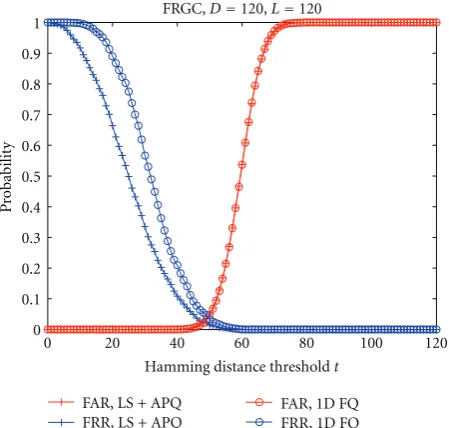
1 FRGC,D=120,L=120
Hamming distance thresholdt
P
robabilit
y
FAR, LS + APQ FRR, LS + APQ
FAR, 1D FQ FRR, 1D FQ
Figure17: An example of the FAR/FRR performances of LS + APQ
and 1D FQ, atD=120,L=120 for FRGC.
formed theL-bit target binary string Sω. Both Sω and the
quantization information ({c∗ω,k},{ϕ∗ω,k}) were stored for
each genuine user. (3) In the verification step, the features of the query user were quantized and coded according to the quantization information ({c∗ω,k},{ϕ∗ω,k}) of the claimed
identity, leading to a query binary string S. Finally, the decision was made by comparing the Hamming distance between the query and the target string.
4.2. Simplified APQ. In practice, computing the optimal offset angleϕ∗ωfor APQ in (7) is difficult, because it is hard to
find a closed-form solutionϕ∗ω. Besides, it is often impossible
to accurately estimate the underlying genuine user PDF pω, due to the limited number of available samples per
user. Therefore, instead ofϕ∗ω, we propose an approximate
solution ϕω. For genuine userω, let the mean of the
two-dimensional feature vector be{μω,1,μω,2}, and its phase be θω = angle(μω,1,μω,2), the approximate offset angle ϕω is
then computed as
ϕω=θω−ξ2, (18)
whereξ = 2π/2b. We give an illustration of computingϕ
ω
inFigure 10. The approximate solutionϕωin fact maximizes
the product of two Euclidean distances, namely, the distance of the mean vector {μω,1,μω,2} to both the lower and the higher genuine interval boundaries.
Note that when the two features have independent Gaussian density with equal standard deviation, ϕ∗ω = ϕω.
Thus, in that case, the simplified APQ equals the original APQ. InFigure 11, we illustrates an example of the detection rate ratio between the simplified and the original APQ, where both features are modeled as Gaussian with different standard deviations, for example, σω,1 = 0.2,σω,2 = 0.8.
The white pixels represent high values whilst the black pixels represent low values. Results show that the simplified APQ is only slightly worse than the original APQ when the mean of the two-dimensional feature{μω,1,μω,2}is close to the origin. However, if we apply APQ after the LS pairing, we would expect that the overall selected pairwise features are located farther away from the origin. In such cases, the simplified APQ works almost the same as the original APQ. InFigure 12 we illustrate the differences of the rotation angle between the original APQ and the simplified APQ, computed from (7) and (18), respectively. These differences are computed from 50 feature pairs for both FVC2000 and FRGC. The results show that there is no much differences between the rotation angle. Additionally, the simplified APQ is much simpler, avoiding the problem of estimating the underlying genuine user PDF pω. For these reasons, we employed this
simplified APQ in all the following experiments (Section 4.3 toSection 4.5).
4.3. APQ d-δ Property. In this section we test the relation between the APQ detection rateδωand the pairwise feature’s
distancedωon both data sets. The goal is to see whether the
real data exhibit the samedω−δωproperty as we found with
synthetic data inSection 2.2: the feature pairs with higherdω
obtains higher detection rateδω.
During the enrollment, for every genuine user, we conducted a random pairing. For every feature pair, we computed theirdωvalue according to (11). Afterwards, we
applied the b-bit APQ quantizer to every feature pair. In the verification, for every feature pair, we computed the Hamming distance between the b-bits from the genuine user and the b-bits from the imposters; that is, we count as a detection if the b-bit genuine query string obtains zero Hamming distance as compared to the target string. Similarly, we count as a false acceptance if theb-bit imposter query string obtains zero Hamming distance as compared to the target string. We then repeated this process over all feature pairs as well as all genuine users, in order to ensure that the results we obtain are neither user or feature biased. Finally, inFigure 13, we plot the relations between thedωand
theδω. The points we plot are averaged according to the bins
ofdω, whenb =2. Results show that for the real data, the
largerdωis, consistently the higher detection rate we obtain.
Additionally, the FAR performance is indeed independent of pairing and equals the theoretical value 2−b.
4.4. LS Pairing Performance. In this section we test the LS pairing performances. We give an example of FVC2000 at D=50.Figure 14(a)shows the histogram ofdfor all single features over all the genuine users. Around 70% of them are close to zero, suggesting low quality features. After LS pairing, the histogram of the pairwised values are shown
in Figure 14(b), as compared with the random pairing. In
−3 −2 −1 0 1 2 3
−3
−2
−1 0 1 2 3
F
eatur
e
v2
Featurev1
Background Genuine user
(a)
0 0.05 0.1 0.15 0.2 0.25 0.3
0.35 Feature densityv1
v1
−3 −2 −1 0 1 2 3
Background Genuine user
(b)
0.4 0.45 0.5
Feature densityv2
Background Genuine user
−3 −2 −1 0 1 2 3
v2
0 0.05 0.1 0.15 0.2 0.25 0.3 0.35
(c)
0 0.1 0.2 0.3 0.4 0.5 0.6 0.7 0.8 0.9 1
Feature densityθ
0 1 2 3 4 5 6
θ
Background Genuine user
(d)
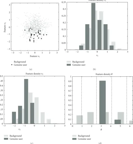
Figure18: An example of the feature density based on LS pairing and APQ. (a) The two-dimensional feature density; (b) the density ofv1;
(c) the density ofv2; (d) the pairwise phase density of{v1v2}, with the adaptive quantization boundaries (dashed line).
“size” densities and moderatedvalues. Thus it avoids small dvalues and effectively maximizes (16).
4.5. Verification Performance. We test the performances of LS + APQ at various numbers of input features Das well as various numbers of quantization bits b ∈ {1,. . ., 6}. The performances are further compared with the one-dimensional fixed quantization (1D FQ) [17]. The EER results for FVC2000 and FRGC are shown in Table 3 and Figure 15.
Table3: The EER performances of LS + APQ and 1D FQ, at various feature dimensionalityDand various numbers of quantization bitsb, for (a) FVC2000 and (b) FRGC.
(a)
FVC2000 DPCA=D, EER=(%)
D=50 100 150 200 250 300
LS + APQ
b=1 4.4 2.8 2.0 1.9 1.8 1.9
b=2 4.6 3.0 2.0 2.1 1.7 1.6
b=3 6.4 3.7 2.8 2.6 2.5 2.7
b=4 8.2 5.9 4.6 3.4 3.2 3.3
b=5 10.0 6.6 5.9 4.4 4.0 3.7
b=6 11.4 7.1 6.6 5.4 4.7 4.7
1D FQ
b=1 6.7 4.0 2.9 2.6 2.7 2.3
b=2 7.5 5.3 4.2 3.6 3.6 3.6
b=3 9.2 6.4 5.5 5.0 5.2 4.9
(b)
FRGC DPCA=500,DLDA=D, EER=(%)
D=50 80 100 120 150 180 200
LS + APQ
b=1 4.0 3.4 3.0 2.6 2.9 2.7 2.7
b=2 3.5 3.0 2.8 2.3 2.8 2.7 2.9
b=3 4.7 4.1 3.7 3.4 3.3 3.6 3.9
b=4 6.7 5.9 5.0 4.8 4.7 5.0 5.2
b=5 8.1 7.0 6.3 6.1 6.5 6.6 6.4
b=6 10.1 8.6 7.5 7.2 7.2 7.4 7.6
1D FQ
b=1 5.7 4.7 4.2 4.0 4.1 4.1 4.2
b=2 5.1 5.4 5.1 5.0 5.2 5.9 6.1
b=3 6.5 6.5 6.4 6.2 6.5 6.9 7.3
Table4: The FAR/FRR performances for FVC2000 and FRGC at
the bestD-Lsetting.
FRR (%) FAR=10−4 10−3 10−2 FVC2000,D=300,L=300 17.2 9.6 2.6 FRGC,D=120,L=120 14.7 8.2 3.7
We further compare the LS + APQ with the 1D FQ. In order to compare at the same string length, we compare the b/2-bit 1D FQ with the b-bit LS + APQ. The EER performances inFigure 15show that in general whenb≤3, LS + APQ outperforms 1D FQ. However, whenb≥4, LS + APQ is no longer competitive to 1D FQ. InFigure 17, we give an example of comparing the FAR/FRR performances of LS + APQ and 1D FQ, on FRGC. Since both APQ and FQ provide equal-probability intervals, they yield almost the same FAR performance. On the other hand, LS + APQ obtains lower FRR as compared with 1D FQ.
In [19], it was shown that FQ in combination with the DROBA adaptive bit allocation principle (FQ + DROBA) provides considerably good performances. Therefore, we compare the LS + APQ with the FQ + DROBA. In order to compare both methods at the sameD-Lsetting, for LS
Table5: The EER performances of LS + APQ and FQ + DROBA, at
at severalD-Lsettings, for (a) FVC2000 and (b) FRGC.
(a)
FVC2000 D=250, EER=(%)
L=50 L=100 L=150
LS + APQ 2.3 1.7 1.9
FQ + DROBA 2.4 2.1 2.2
(b)
FRGC D=120, EER=(%)
L=60 L=90 L=120
LS + APQ 2.3 2.4 2.3
FQ + DROBA 2.4 2.6 2.8
+ APQ, we extract only 2K features from the D features, thusKpairs from the LS pairing. Afterwards, we apply the 2-bit APQ for every feature pair (seeFigure 3). In this case,
K =L/2.Table 5shows the EER performances of LS + APQ
5. Discussion
Essentially, the pairwise phase quantization involves two user-specific adaptation steps: the long-short (LS) pairing, as well as the adaptive phase quantization (APQ). From the pairing’s perspective, although we only quantize the phase, the magnitude information (i.e. the feature mean) is not discarded. Instead, it is employed in the LS pairing strategy to facilitate extracting distinctive phase bits. Additionally, although with low computational complexity, the LS pairing strategy is effective for arbitrary feature densities. From the quantizer’s perspective, quantizing in phase domain has the advantage that a circularly symmetric two-dimensional feature density results in a simple uniform phase density. Additionally, we apply user-specific phase adaptation. As a result, the extracted phase bits are not only distinctive but also robust to over-fitting. However, the experimental results imply that such advantages only exist when b ≤ 3. To summarize, as illustrated in Figure 18, the LS pairing is a user-specific resampling procedure that provides simple unform but distinctive phase densities. The APQ further enhances the feature distinctiveness by adjusting the user-specific phase quantization intervals.
6. Conclusion
Extracting binary biometric strings is a fundamental step in biometric compression and template protection. Unlike many previous work which quantize features individually, in this paper, we propose a pairwise adaptive phase quan-tization (APQ), together with a long-short (LS) pairing strategy, which aims to maximize the overall detection rate. Experimental results on the FVC2000 and the FRGC database show reasonably good verification performances.
Acknowledgment
This research is supported by the research program Sentinels (http://www.sentinels.nl/). Sentinels is being financed by Technology Foundation STW, the Netherlands Organization for Scientific Research (NWO), and the Dutch Ministry of Economic Affairs.
References
[1] A. K. Jain, K. Nandakumar, and A. Nagar, “Biometric template security,”EURASIP Journal on Advances in Signal Processing, vol. 2008, Article ID 579416, 2008.
[2] N. K. Ratha, J. H. Connell, and R. M. Bolle, “Enhancing secu-rity and privacy in biometrics-based authentication systems,” IBM Systems Journal, vol. 40, no. 3, pp. 614–634, 2001. [3] N. K. Ratha, S. Chikkerur, J. H. Connell, and R. M. Bolle,
“Generating cancelable fingerprint templates,”IEEE Transac-tions on Pattern Analysis and Machine Intelligence, vol. 29, no. 4, pp. 561–572, 2007.
[4] A. Juels and M. Sudan, “A fuzzy vault scheme,”Designs, Codes, and Cryptography, vol. 38, no. 2, pp. 237–257, 2006.
[5] K. Nandakumar, A. K. Jain, and S. Pankanti, “Fingerprint-based fuzzy vault: implementation and performance,”IEEE
Transactions on Information Forensics and Security, vol. 2, no. 4, pp. 744–757, 2007.
[6] A. Juels and M. Wattenberg, “Fuzzy commitment scheme,” in Proceedings of the 6th ACM Conference on Computer and Communications Security (ACM CCS ’99), pp. 28–36, November 1999.
[7] Y. Dodis, L. Reyzin, and A. Smith, “Fuzzy extractors: how to generate strong keys from biometrics and other noisy data,” inProceedings of International Conference on the Theory and Applications of Cryptographic Techniques, vol. 3027 ofLecture Notes in Computer Science, pp. 523–540, May 2004.
[8] E. C. Chang and S. Roy, “Robust extraction of secret bits from minutiae,” inProceedings of the 2nd International Conference on Biometrics (ICB ’07), vol. 4642 ofLecture Notes in Computer Science, pp. 750–759, 2007.
[9] J.-P. Linnartz and P. Tuyls, “New shielding functions to enhance privacy and prevent misuse of biometrie templates,” in Proceedings of Audio-and Video-Based Biometrie Person Authentication (AVBPA ’03), vol. 2688 of Lecture Notes in Computer Science, pp. 393–402, Guildford, UK, 2003. [10] P. Tuyls, A. H. M. Akkermans, T. A. M. Kevenaar, G.-J.
Schri-jen, A. M. Bazen, and R. N. J. Veldhuis, “Practical biometric authentication with template protection,” in Proceedings of the 5th International Conference on Audio-and Video-Based Biometric Person Authentication (AVBPA ’05), vol. 3546 of Lecture Notes in Computer Science, pp. 436–446, Hilton Rye Town, NY, USA, July 2005.
[11] T. A. M. Kevenaar, G. J. Schrijen, M. van der Veen, A. H. M. Akkermans, and F. Zuo, “Face recognition with renewable and privacy preserving binary templates,” inProceedings of the 4th IEEE Workshop on Automatic Identification Advanced Technologies (AUTO ID ’05), pp. 21–26, New York, NY, USA, October 2005.
[12] F. Hao, R. Anderson, and J. Daugman, “Combining crypto with biometrics effectively,”IEEE Transactions on Computers, vol. 55, no. 9, pp. 1081–1088, 2006.
[13] A. B. J. Teoh, A. Goh, and D. C. L. Ngo, “Random multispace quantization as an analytic mechanism for BioHashing of biometric and random identity inputs,”IEEE Transactions on Pattern Analysis and Machine Intelligence, vol. 28, no. 12, pp. 1882–1901, 2006.
[14] C. Vielhauer, R. Steinmetz, and A. Mayerh¨ofer, “Biometric hash based on statistical features of online signatures,” in Proceedings of the 16th International Conference on Pattern Recognition (ICPR ’02), vol. 1, pp. 123–126, Quebec, Canada, 2002.
[15] H. Feng and C. C. Wah, “Private key generation from on-line handwritten signatures,” Information Management and Computer Security, vol. 10, no. 4, pp. 159–164, 2002.
[16] Y. -J. Chang, W. Zhang, and T. Chen, “Biometrics-based cryptographic key generation,” in Proceedings of the IEEE International Conference on Multimedia and Expo (ICME ’01), vol. 3, pp. 2203–2206, Taipei, Taiwan, June 2004.
[17] C. Chen, R. N. J. Veldhuis, T. A. M. Kevenaar, and A. H. M. Akkermans, “Multi-bits biometric string generation based on the likelihood ratio,” inProceedings of the 1st IEEE International Conference on Biometrics: Theory, Applications, and Systems (BTAS ’07), September 2007.
[19] C. Chen, R. N. J. Veldhuis, T. A. M. Kevenaar, and A. H. M. Akkermans, “Biometric quantization through detection rate optimized bit allocation,” EURASIP Journal on Advances in Signal Processing, vol. 2009, Article ID 784834, 2009.
[20] C. Chen and R. N. J. Veldhuis, “Extracting biometric binary strings with minimal area under the frr curve for the hamming distance classifier,” inProceedings of the 17th European Signal Processing Conference (EUSIPCO ’09), 2009.
[21] C. Chen and R. Veldhuis, “Binary biometric representation through pairwise polar quantization,” inProceedings of the 3rd International Conference on Advances in Biometrics (ICB ’09), vol. 5558 ofLecture Notes in Computer Science, pp. 72–81, Alghero, Italy, June 2009.
[22] J. Daugman, “The importance of being random: statistical principles of iris recognition,”Pattern Recognition, vol. 36, no. 2, pp. 279–291, 2003.
[23] D. Maio, D. Maltoni, R. Cappelli, J. L. Wayman, and A. K. Jain, “FVC2000: fingerprint verification competition,” IEEE Transactions on Pattern Analysis and Machine Intelligence, vol. 24, no. 3, pp. 402–412, 2002.
[24] P. J. Phillips, P. J. Flynn, T. Scruggs et al., “Overview of the face recognition grand challenge,” inProceedings of IEEE Computer Society Conference on Computer Vision and Pattern Recognition (CVPR ’05), pp. 947–954, San Diego, Calif, USA, June 2005. [25] R. Veldhuis, A. Bazen, J. Kauffman, and P. Hartel, “Biometric
verification based on grip-pattern recognition,” in Security, Steganography, and Watermaking of Multimedia Contents VI, vol. 5306 ofProceedings of SPIE, pp. 634–641, San Jose, Calif, USA, January 2004.