Development of Modified Smith Predictor Design for Compensation of Time Delayed Processes

(1)

International Journal of Research (IJR)

e-ISSN: 2348-6848, p- ISSN: 2348-795X Volume 2, Issue 08, August 2015

Available at http://internationaljournalofresearch.org

Development of Modified Smith Predictor Design for

Compensation of Time Delayed Processes

Sakshi Bangia*

[email protected]

Komal Sharma**

[email protected]

*Assistant professor, YMCA University of Science and Technology, Faridabad **M.tech student, YMCA University of Science and Technology, Faridabad

Abstract:

A time delay may be defined as the time interval between the start of an event at one point in a system and its resulting action at another point in the system. Delays are also known as transport lags or dead times. Delays may arise in a wide variety of process dynamics and manufacturing applications. Traditionally used PID controllers are less effective if the time delay term in the process dynamics is dominant. For such applications, the Smith predictor can give better performance. The Smith predictor structure utilizes a mathematical model of the process in a minor feedback loop. One of its advantages is that the Smith predictor approach for a SISO system may be directly extended to the MIMO system with the same delay. A modification is proposed to the Smith predictor compensator structure for the control of a process with time delay. The modification facilitates the achievement of an improved closed loop system regulator response, with little degradation in the corresponding servo response. This paper presents a technique for analyzing the stability of time-delay systems using modified Smith predictor. Implementation using MATLAB has been made to compare the performance of modified smith predictor with Smith predictive control and PI controller on second order process with time delay.Robustness of the Smith Predictoris verified is to uncertainty on the process dynamics and dead time.

Keywords- Time delay; compensation; Smith predictor; Proportional Integral (PI) Controller; Modified smith predictor; robustness

1. INTRODUCTION

An extensive literature exists on the compensation of time delayed processes. These compensation methods may be broadly divided into parameter optimized controllers, in which the controller parameters are adapted to the controller structure (the most common such controller is the proportional integral derivative, or PID, controller), and structurally optimized controllers, in which the controller structure and parameters are adapted optimally to the structure and parameters of the process model.

In manufacturing applications, delays typically arise whenever there is physical

transport of material, for example, in a pipe or on a conveyer belt; the delay can be determined as the ratio of distance to be traveled to the speed of the material. Delays arise in a wide variety of other manufacturing applications, often in combination with other process dynamics; examples of such applications range from plastic part fabrication to heating, ventilation and air conditioning (HVAC) to industrial sewing machines.

(2)

International Journal of Research (IJR)

applications, more than 90%- 95% of the controllers are of PID type [3-8]. However, PID controllers are less effective if the time delay term in the process dynamics is dominant. For such applications, the Smith predictor can give better performance.

Since the Smith Predictor structure was proposed, many modifications have been proposed to improve the servo response, the regulator response or both. Modifications were accomplished to adapt the structure to stable, integrative or unstable systems. Sourdille and O‟Dwyer [9] present an extensive review of the literature concerning modifications to the Smith predictor; this review was used to develop a generalized form of the predictor. This paper discusses the generalized form of the Smith predictor and a new modified Smith predictor structure with its associated tuning rules.

1.1Design of PI controller, smith predictor and modified smith predictor

1.1.1 PI controller

A proportional-integral (PI controller) is a control loopfeedback mechanism (controller) widely used in industrial control systems. A PI controller calculates an error value as the difference between a measured process variable and a desired setpoint. The controller attempts to minimize the error by adjusting the process through use of a manipulated variable. The PI controller algorithm involves two separate constant parameters, and is accordingly sometimes called three-term control: the proportional and the integral values, denoted P andI. Simply put, these values can be interpreted in terms of time: P depends on the present error, I on the accumulation of past errors, based on current rate of change. The weighted sum of these two actions is used to adjust the process via a control element such as the position of a

control valve, a damper, or the power supplied to a heating element

A control system with proportional and integral control (PI) is shown in Figure 1.

Figure 1: Block diagram of a control system with a PI controller

For a PI controller, the controller output is given by equation (1) in the time domain [1]:

𝑝 𝑡 = 𝑝 +𝐾_𝑐(𝑒 𝑡 + 1

𝜏𝐼 𝑒(𝑡)𝑑𝑡) 𝑡

0

(1)

The corresponding transfer function in the Laplace domain is given by:

𝑃(𝑠)

𝐸(𝑠)= 𝐾𝑐 1 + 1

𝜏_𝐼𝑠

=𝐾𝐶

𝜏_𝐼𝑆+ 1

𝜏𝐼𝑆

(2)

The closed-loop set-point transfer function for the feedback control in Figure 1 is obtained from the following derivation, where the disturbance is assumed to be zero:

Y=GP (3)

P=E𝐺_𝐶 (4) E=𝑌_𝑠𝑝-Y (5)

By inserting equation (4) and (5) into equation (3), the equation becomes

Y=𝐺_𝐶𝐺(𝑌_𝑠𝑝 − 𝑌) (6)

(3)

International Journal of Research (IJR)

Y (1+𝐺_𝑐𝐺) =𝑌_𝑠𝑝𝐺_𝐶𝐺 (7)

This gives the closed-loop transfer function for set-point changes:

𝑌 𝑌𝑠𝑝 =

𝐺𝑐𝐺

1+𝐺𝑐𝐺 (8)

When the process has a time delay, the process transfer function is given by

G=𝐺𝑛𝑒−𝜃𝑠(9)

Finally the closed-loop set-point transfer function is given as:

𝑌 𝑌𝑠𝑝 =

𝐺𝑐𝐺𝑛𝑒−𝜃𝑠

1+𝐺𝑐𝐺𝑛𝑒−𝜃𝑠 (10)

1.1.2 Smith predictor:

The design of controllers for processes with long time delays has been of interest to academics and practitioners for several decades. In a seminal contribution, Smith [1] proposed a technique that reduces the dominance of the delay term in the closed loop characteristic equation; a „primary‟ controller may then be designed for the non-dominant delay process. This method, called the Smith predictor, has been the subject of numerous experimental and theoretical studies. A block diagram of the Smith predictor is provided in Figure1.The Smith predictor is the optimal controller for a delayed process for servo applications, or for a step disturbance, if the optimal controller is designed using a constrained minimum output variance control law. If the disturbance is not of step form, then the optimal controller may be specified for regulator applications by the inclusion of an appropriate dynamic element in the feedback path of the Smith predictor structure [12]. The Smith predictor may also be related to other delay compensator

strategies [13]. The main problem with controlling dead-time systems is associated with the time lapse before the effect of the disturbances, or the control actions, are experienced. The controller will be attempting to correct a situation that happened backwards in time. A predictor correction structure can improve the performance of closed-loop systems with significant time-delay.

The Smith predictor consists of a regular controller and a model of the dead time process that is to be controlled. The purpose of the Smith predictor is to allow the controller to observe the expected process response before it occurs, thus cancelling the effect of the delay on the closed loop dynamics.

The Smith predictor can achieve improved control of processes with delay, some unintuitive behavior is observed when there is modeling mismatch between the time-delay in the process and the process model used by the Smith predictor. Instability is reported in some cases when the real time-delay is less than the modeled time-delay. As Smith predictors often are designed using an overestimated delay, discontinuities in the stability domain can pose serious service problems. Smith predictor control is one of several strategies that have been developed to improve the performance of systems containing time delays [11]. It is desirable to achieve effective time-delay compensation with these methods. The experiments have shown that the Smith predictor gives a better performance than a conventional PI controller [11].

(4)

International Journal of Research (IJR)

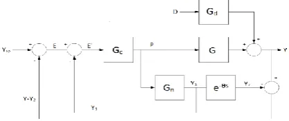
Figure 2: Block diagram for a process with the Smith predictor controller.

As seen in Figure 1, the Smith predictor structure can be divided into two parts. This includes the primary controller, GC(s), and the

predictor structure. The predictor part consists of a model of the plant without time delay (Gn(s)), and a model of the time delay (e-θs)

[10]. The parameter θ is the time delay. Thus, the complete process model is given by equation (11).

𝑃_𝑛 𝑠 =𝐺_𝑛(𝑠)𝑒−𝜃𝑠₍₁₁₎

The model without the dead-time is sometimes called the fast model and is used to compute an open-loop prediction. Thus, the model of the process without time delay (Gn)

is used to predict the effect of control actions on the un-delayed output [11]. Then the controller uses the predicted response (Y1) to

calculate its output signal (P). The actual un-delayed output (Y) is compared with the delayed predicted output (Y2). In the case of

no disturbances or modeling errors, the difference between the process output and the model output will be zero. This means that the output signal (Y-Y2) will be equal to the

output of the plant without any time delay [9].

Derivation of Transfer Function for Inner Feedback Loop-

The block diagram for the Smith predictor given in Figure 2 can be re-drawn as two nested feedback loops as shown in Figure 3.

Figure 3: The Smith Predictor block diagram re-drawn as two nested feedback loops.

To find the equivalent transfer function for the inner feedback loop in Figure 3, an expression for P/E is needed. This function is derived by using the blocks in Figure 3. The goal is to find G‟, given by:

𝐺 = 𝑃

𝐸 12

Investigation of the block diagram in Figure 3 gives the following:

𝑃 =𝐸 𝐺𝑐 (13)

𝐸 = 𝐸 − 𝑌₁− 𝑌₂ (14)

𝑌₁− 𝑌₂ =𝑃𝐺_𝑛 1

− 𝑒−𝜃𝑠 ₍₁₅₎

By inserting equation (15) and (16) into (14), the equation becomes:

𝑃

= 𝐸

− 𝑃𝐺_𝑛 1− 𝑒−𝜃𝑠_𝐺

𝑐 (16)

Simplifying equation (17) gives

𝑃 1 +𝐺𝑐𝐺𝑛 1− 𝑒−𝜃𝑠

=𝐸𝐺_𝑐 (17)

The transfer function for the inner feedback loop in Figure 3 is then obtained:

𝐺 =𝑃

𝐸 =

𝐺_𝑐

1 +𝐺_𝑐𝐺_𝑛(1− 𝑒−𝜃𝑠₎ (18)

By doing some rearrangement, the closed-loop set-point transfer function for the Smith predictor is given by:

𝑌 𝑌_𝑠𝑝 =

𝐺𝑐𝐺𝑛𝑒−𝜃𝑠

1 +𝐺_𝑐𝐺_𝑛 (19)

(5)

International Journal of Research (IJR)

missing from the characteristic equation of the Smith predictor controller, but it is present in the closed-loop set-point transfer function of the PI controller. The characteristic equation is the denominator part of the closed-loop set-point transfer function for a given controller. This gives a theoretical explanation of the time delay compensating ability of the Smith predictor.

1.1.3 Modified Smith predictor

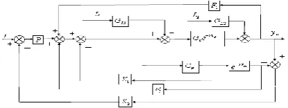
A number of authors have proposed modifications to the Smith predictor structure to improve the regulator response of the compensated system and/or to reduce the effect on either the servo or the regulator response of process-model mismatch. Many of the modifications of the Smith predictor structure discussed are subsets of the implementation provided in Figure 4 below.

Figure 4 modified smith predictor structure

The response of the above system may be derived to be

yp =

(GpPe−sτp)r+1+GmK1+F2−K2Pe−sτm (GL 2L2+GpGL 1e−sτpL1)

1+GmK1+Gm F2−K2Pe−sτm−GpF1−K2Pe−sτp

(20)

One may optimize the servo and regulator responses, and minimize the effect of the mismatch between the process and the model, by appropriate design of three of the five dynamic elements in Figure 2. It may be shown that five separate modifications to the Smith predictor structure may be defined theoretically such that ideal servo and regulator action is achieved, with elimination

of process-model mismatch, under the assumption that the unknown process parameters are represented by appropriate known model parameters. Unfortunately, all of the implementations require the inversion of the model transfer function and/or the time delay to set up one of the required dynamic elements. Such non-proper transfer functions would need to be approximated, which provokes instability in the resulting compensated system. It was decided to design a modified Smith predictor to achieve a servo response similar to that obtained from an open-loop first order lag plus delay (FOLPD) model, with a corresponding regulator response. Such responses may also be achieved by using the Internal Model Control (IMC) strategy described by Morari and Zafiriou [14]. Six separate modifications to the Smith predictor strategy may be defined that will facilitate the desired servo and regulator action, with process-model mismatch elimination, provided the process parameters are known. More realistically, the process parameters are normally unknown; if the process is represented by a known model, then four such modifications to the Smith predictor strategy can be used. Such modifications will not facilitate the complete elimination of process-model mismatch.

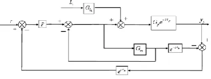
With 𝑏= 𝐺_𝑐(1 +𝐺_𝑚)/(1 +𝐺_𝑐𝐺_𝑚) (21)

If Gmis a first order lag element and Gcis a PI controller, then the best modification to choose is when P=b, F1=F2=0, K1=1 and K2=𝑒𝑠𝜏𝑚_{, as the only non-proper dynamic}

(6)

International Journal of Research (IJR)

Figure 5: Block diagram of the modified Smith predictor structure chosen

This structure has interesting similarities with the structures defined by Hockenet al. [15] (who approximate the extra dynamic element by a time delay equal to the difference between the process and model time delays) and Romagnoliet al. [16] (who use a lag controller dynamic element). However, a better approximation of the time advance is provided by Huang et al. [17], as follows:

𝑒𝜏𝑚𝑠 _≈ 1+𝐵(𝑠)

1+𝐵(𝑠)𝑒−𝑠𝜏𝑚

(22)

𝐵 𝑠 = 𝑘

1+𝑇𝑠

(23)

The time advance approximation may be improved by defining B(s) as a phase lead network i.e. B(s) = (as + 1)/ (as + p), p > 1. The servo and regulator responses, using the approximation, are as indicated below.

𝑦𝑝 𝑟 =

𝐺𝑝𝐺𝑐𝑒−𝑠𝜏𝑝

1+𝐺𝑐𝐺𝑚+𝐺𝑐 ₁₊_{𝐵 𝑠 𝑒−𝑠𝜏𝑚}1+𝐵 𝑠 𝐺𝑝𝑒−𝑠𝜏𝑝−𝐺𝑚𝑒−𝑠𝜏𝑚

(23)

𝑦𝑝 𝐿1=

𝐺𝑝𝑒−𝑠𝜏𝑝1+𝐺𝑚𝐺𝑐 1−𝑒−𝑠𝜏𝑚 +𝐵 𝑠 𝑒−𝑠𝜏𝑚

1+𝐺𝑐𝐺𝑚 1+𝐵 𝑠 𝑒−𝑠𝜏𝑚 +𝐺𝑝 1+𝐵 𝑠 𝐺𝑝𝑒−𝑠𝜏𝑝−𝐺𝑚𝑒−𝑠𝜏𝑚

(24)

2. Results and Discussion

2.1Process model

The process open-loop response is modeled as a second-order plus dead time with a 1 second time delay. The transfer function is given by:

exp −1∗s ∗ 1

. 05∗s2 _{+ .6}_∗_{s + 1}

The step response of the open loop process is shown below in Figure 6.

Figure 6. Step response of spring mass damper system

2.1.1 PI controller:

Proportional-Integral (PI) control is a commonly used technique in Process Control. The PI compensator C consists of a proportional gain Kp and integrator time

constant Ti:

𝐶 𝑠 = 𝐾_𝑝(1 + 1

𝑇𝑖𝑠)

(25)

There are many guidelines for choosing the 𝐾_𝑝

and𝑇_𝑖 parameters. But here we use Ziegler Nicholous tuning rules for finding the value of

𝐾_𝑝and 𝑇_𝑖

𝐾_𝑝 = 0.6

𝑇𝑖 = 1

To evaluate the performance of the PI controller, close the feedback loop is closed and the responses to step changes is simulated in the reference signal ysp and disturbance

(7)

International Journal of Research (IJR)

Figure 7 Step response of the process with PI controller

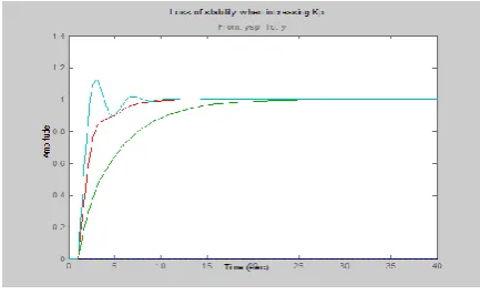
The closed-loop response obtained has acceptable overshoot but is somewhat sluggish (it settles in about 10 seconds). Increasing the proportional gain 𝐾𝑝 speeds up the response

but also significantly increases overshoot and quickly lead to instability as shown in Figure 8.

Figure 8 Effect of increasing the value of proportional gain

2.2 Comparison of PI controller with Smith Predictor

To compare the performance of the two designs, first derive the closed-loop transfer function from ysp, dto y for the Smith

Predictor architecture.

Figure 9 Comparison of step response of PI controller vs smith predictor

The Smith Predictor provides much faster response with no overshoot. The difference is also visible in the frequency domain by plotting the closed-loop Bode response from ysp to y. The higher bandwidth for the Smith

Predictor is shown in Figure 10.

Figure 10 Comparison of Bode plot of PI controller vs smith predictor

2.3 Robustness to model mismatch

In the previous analysis, the internal model

𝐺_𝑝(𝑠)𝑒−𝜏𝑠

Matched the process model P exactly. In practical situations, the internal model is only an approximation of the true process dynamics, so it is important to understand how robust the Smith Predictor is to uncertainty on the process dynamics and dead time.

Consider two perturbed plant models representative of the range of uncertainty on the process parameters:

𝑃1=𝑒−1𝑠

1

. 01𝑠+ 1 . 3𝑠+ 1

𝑃2=𝑒−2𝑠

1

(8)

International Journal of Research (IJR)

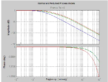
Figure 11 Bode plot of nominal and perturbed process model

To analyze robustness, collect the nominal and perturbed models into an array of process models, rebuild the closed-loop transfer functions for the PI and Smith Predictor designs, and thus bode response and the closed-loop responses is simulated, as shown in Figure 11 and Figure 12 respectively.

Figure 12 Comparison of step response of PI controller vs smith predictor of nominal and

perturbed process model

Both designs are sensitive to model mismatch, as confirmed by the closed-loop Bode plots.Comparison of Bode plot of PI controller vs smith predictor of nominal and perturbed process model is shown in Figure 13.

Figure 13 Comparison of Bode plot of PI controller vs smith predictor of nominal and

perturbed process model

2.3Improving Robustness

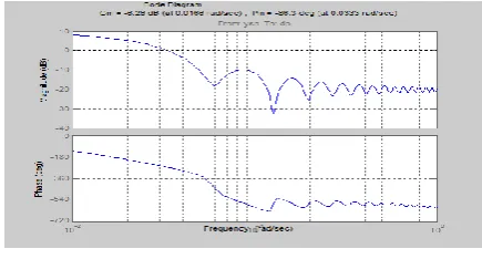
To reduce the Smith Predictor's sensitivity to modeling errors, check the stability margins for the inner and outer loops. The inner loop C has open-loop transfer C*Gp so the stability margin are obtained as shown in Figure 14.

Figure 14 Stability margin of inner loop

The inner loop has comfortable gain and phase margins so focus on the outer loop next. The open-loop transfer function has been derived.

(9)

International Journal of Research (IJR)

Note the -300dB gain: this transfer function is essentially zero, which is to be expected when the process and prediction models match exactly. To get insight into the stability margins for the outer loop, we need to work with one of the perturbed process models, e.g., P1:

Figure 16 Improved Boderesponse with the help of filter

This gain curve has a hump near 0.07 rad/s as shown in Figure 17 that lowers the gain margin and increases the hump in the closed-loop step response. To fix this issue, pick a filter F that rolls off earlier and more quickly.

Figure 17 Improved Boderesponse by making changes in filter

Finally, the closed-loop responses with the modified filter is simulated in Figure 18.

Figure 18 Comparison of modified filter vs PI controller

The modified design provides more consistent performance at the expense of a slightly slower nominal response.

2.4Comparison of PI controller, smith predictor and modified smith predictor:

A Comparison of PI controller vs smith predictor vs modified smith predictor has been shown inFigure 19.

Figure 19 Comparison of PI controller vs smith predictor vs modified smith predictor

This comparison shows that our last design speeds up disturbance rejection at the expense of slower setpoint tracking.

3. Conclusion

(10)

International Journal of Research (IJR)

an extensive literature review, a generalized Smith predictor structure is developed. A modification to the conventional Smith predictor structure for the control of a process with time delay has been proposed to facilitate the achievement of a modest improvement in the closed loop system responses. The modification involves approximating a time advance term that may be incorporated in the outer feedback loop of the predictor. A modified Smith predictor structure is subsequently developed with the aim of achieving excellent servo and regulator responses. From the implementation of this structure, it may be concluded that better regulator responses are achieved in the vast majority of cases when the modified Smith predictor is used instead of the corresponding Smith predictor.

4. REFERENCES

[1.] Smith, O.J.M. (1957)”Closer control of loops with dead time”, Chemical

Engineering Progress, 53, 217-219.

[2.] O‟Dwyer, A. “Handbook of PI and

PID controller tuning rules.” London,

U.K.: Imperial College Press, 2003.

[3.] Astrom, K.J. and Hagglund, T. (1995).

“PID controllers: theory, design and

tuning,” Second Edition, Instrument

Society of America.

[4.] Koivo, H.N. and Tanttu, J.T. (1991).

“Proc. IFAC Intelligent Tuning Adaptive

Control Symp.,“Singapore, 75.

[5.] Bialkowski, W.L. (1996), in “The

Control Handbook, W.S Levine, Ed. Boca

Raton, Florida”, CRC/IEEE Press, 1219.

[6.] Luyben, W.L. and Luyben, M.L. (1997) “Essentials of process control.” Singapore: McGraw-Hill International Edition.

[7.] Hersh, M.A, and M.A. Johnson, M.A. (1997), Control Eng. Practice, 5(6), 771.

[8.] Takatsu, T. and Itoh, T. (1999), IEEE

Trans. Control Syst. Tech., 7(3), 298.

[9.] Sourdille, P. and O‟Dwyer, A. (2003),”An outline and further development of Smith predictor based methods for the compensation of processes with time delay”, Irish Signals and Systems Conference 2003.

[10.] Hang, C.C. and Wong, F.S. (1979) “Modified Smith predictors for the control of processes with dead time, Proceedings of the ISA Conference and Exhibition”

Advances in Instrumentation and Control,

34, 2, 33-44, Chicago, IL., U.S.A.

[11.] Seborg, D.E., Edgar, T.F. and Mellichamp, D.A. (1989)”Process

dynamics and control”, John Wiley and

Sons.

[12.] Gorecki, R. and Jekielek, J. (1997)” Simplifying controller for process control of systems with large dead time”,Proceedings of the ISA Tech/Expo

Technology Update, Anaheim, California,

1, 5, 113-120.

(11)

International Journal of Research (IJR)

Instrumentation, Houston, Texas, U.S.A.,

35, 1, 57-68.

[14.] Morari, M. and Zafiriou, E., “Robust

process control”, Prentice-Hall Inc., 1989.

[15.] Hocken, R.D., Salehi, S.V. and Marshall, J.E. “Time-delay mismatch and the performance of predictor control schemes”, International Journal of

Control, Vol. 38, pages 433-447, 1983.

[16.] Romagnoli, J.A., Karim, M.N., Agamennoni, O.E. and Desages, A., “Controller designs for model-plant parameter mismatch”, IEE Proceedings

Part D, Vol. 135, No. 2, pages 157-164,

March 1988.

[17.] 17. Huang, H.-P., Chen, C.-L., Chao, Y.-C. and Chen, P.-L., “A modified Smith predictor with an approximate inverse of dead time”, AIChE Journal, Vol. 36, No. 7, pages 1025-1031, July 1990