Merge Sort Algorithm
Jaiveer Singh (16915) & Raju Singh(16930)
Department of Information and Technology Dronacharya College of Engineering Gurgaon, India
[email protected] ; [email protected]
ABSTRACT:
Given an array with n elements, we want to rearrange them in ascending order. Sorting algorithms such as the Bubble, Insertion and Selection Sort all have a quadratic time complexity that limits their use when the number of elements is very big. In this paper, we introduce Merge Sort, a divide-and- conquer algorithm to sort an N element array. We evaluate the O(NlogN) time complexity of merge sort theoretically and empirically. Our results show a large improvement in efficiency over other algorithms.
1. INTRODUCTION
Search engine is basically using sorting algorithm. When you search some key word online, the feedback information is brought to you sorted by the importance of the web page. Bubble, Selection and Insertion Sort, they all have an O(N2) time complexity that limits its usefulness to small number of element no more than a few thousand data points. The quadratic time complexity of existing algorithms such as Bubble, Selection and Insertion Sort limits their performance when array size increases. In this paper we introduce Merge Sort which is able to rearrange elements of a list in ascending order. Merge sort works as a
array elements in O(NlogN) time. We evaluate the O(NlogN) time complexity theoretically and empirically. The next section describes some existing sorting algorithms: Bubble Sort, Insertion Sort and Selection Sort. Section 3 provides a details explanation of our Merge Sort algorithm. Section 4 and 5 discusses empirical and theoretical evaluation based on efficiency. Section 6 summarizes our study and gives a conclusion.
Note: Arrays we mentioned in this article have the size of N.
2. RELATED WORK
Selection sort [1] works as follows: At each iteration, we identify two regions, sorted region (no element from start) and unsorted region. We “select” one smallest element from the unsorted region and put it in the sorted region. The number of elements in sorted region will increase by 1 each iteration. Repeat this on the rest of the unsorted region until it isexhausted. This method is called selection sort because it works by repeatedly “selecting” the smallest remaining element.
the first element. Experiments by Astrachan [4] sorting strings in Java show bubble sort is roughly 5 times slower than insertion sort and 40% slower than selection sort which shows that Insertion is the fastest among the three. We will evaluate insertion sort compared with merge sort in empirical evaluation.
Bubble sort works as follows: keep passing through the list, exchanging adjacent element, if the list is out of order; when no exchanges are required on some pass, the list is sorted.
In Bubble sort, Selection sort and Insertion sort, the O(N2) time complexity limits the performance when N gets very big. We will introduce a “divide and conquer” algorithm to lower the time complexity.
3. APPROACH
Merge sort uses a divide-and-conquer approach:
1) Divide the array repeatedly into two halves
2) Stop dividing when there is single element left. By fact, single element is already sorted.
3) Merges two already sorted sub arrays into one. Pseudo Code:
a) Input: Array A[1…N], indices p, q, r (p ≤ q <r). A[p…r] is the array to be divided A[p] is the beginning element and A[r] is the ending element Output: Array A[p…r] in ascending order
4. Theoretical Evaluation
Comparison between two array elements is the key operation of bubble sort and merge sort. Because before we sort the array we need to compare between array elements. The worst case for merge sort occurs when we merge two sub arrays into one if the biggest and the second biggest elements are in two separated sub array. Let N=8, we have array {1,3,2,9,5,7,6,8,}. From figure 1.a, element 3(second biggest element),9(biggest element) are in separated sub array. # of comparisons is 3 when {1,3} and {2,9} were merged into one array. It’s the same case merge {5,7} and {6,8} into one array.
From figure 1.b, 9,8 are in separated sub array, we can see after 3 comparisons element 1,2,3 are in the right place. Then
Let T(N)=# of comparison of merge sort n array element. In the worst case, # of comparison of last merge is
N-1. Before we merge two N/2 sub arrays into one, we need to sort them. It took 2T(N/2). We have
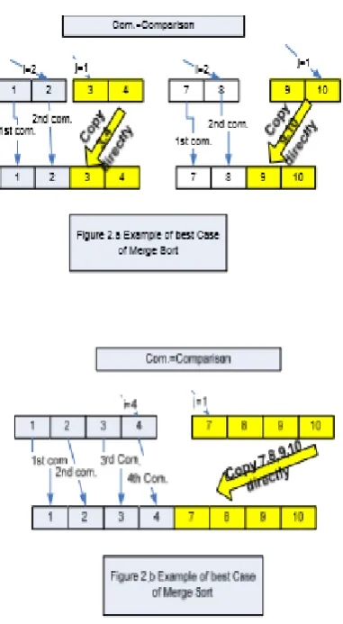
From figure 2.b, we can see after 4 comparisons, element 1,2,3,4 are in the right place. The last comparison occurs when i=4, j=1. Then 7,8,9,10 are copied to the right place directly. # of comparisons is only 4(half of the array size)
Let T(N)=# of comparison of merge sort n array element. In the worst case, # of comparison of last merge is N/2. We have
5.Empirical Evaluation
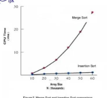
The efficiency of the merge sort algorithm will be measured in CPU time which is measured using the system clock on a machine with minimal background processes running, with respect to the size of the input array, and compared to the selection sort algorithm. The merge sort algorithm will be run with the array size parameter set to: 10k, 20k, 30k, 40k, 50k and 60k over a range of varying-size arrays. To ensure reproducibility, all datasets and algorithms used in this evaluation can be
found at
“http://cs.fit.edu/~pkc/pub/classes/writing/ht tpdJan24.log.zip”. The data sets used are synthetic data sets of varying-length arrays with random numbers. The tests were run on PC running Windows XP and the following specifications: Intel Core 2 Duo CPU E8400 at 3.00 GHz with 2 GB of RAM. Algorithms are run in Java.
5.1 Procedures
The procedure is as follows: 1 Store 60,000 records in an array 2 Choose 10,000 records 3 Sort records using merge sort and insertion sort algorithm 4 Record CPU time 5 Increment Array size by 10,000 each time until reach 60,000, repeat 3-5
5.2 Results and Analysis
Table 1 shows Merge Sort is slightly faster than Insertion Sort when array size N (3000 - 7000) is small. This is because Merge Sort has too many recursive calls and temporary array allocation.
By passing the paired t-test using data in table 1, we found that difference between merge and insertion sort is statistically significant with 95% confident. (t=2.26, d.f.=9, p<0.05)
6. Conclusions
In this paper we introduced Merge Sort algorithm, a O(NlongN) time and accurate
theoretical and empirical analysis showed that Merge sort has a O(NlogN) time complexity. Merge Sort’s efficiency was compared with Insertion sort which is better than Bubble and Selection Sort. Merge sort is slightly faster than insertion sort when N is small but is much faster as N grows. One of the limitations is the algorithm must copy the result placed into Result list back into m list(m list return value of merge sort function each call) on each call of merge . An alternative to this copying is to associate a new field of information with each element in m. This field will be used to link the keys and any associated information together in a sorted list (a key and its related information is called a record). Then the merging of the sorted lists proceeds by changing the link values; no records need to be moved at all. A field which contains only a link will generally be smaller than an entire record so less space will also be used. REFERENCES
[1] Sedgewick, Algorithms in C++, pp.96‐9 8, 102, ISBN 0‐201‐
51059‐6 ,Addison‐Wesley , 1992 [2] Sedgewick, Algorithms in C++, pp.98‐1 00, ISBN 0‐201‐51059‐
6 ,Addison‐Wesley , 1992
[3] Sedgewick, Algorithms in C++, pp.100‐104, ISBN 0‐201‐
51059‐6 ,Addison‐Wesley , 1992