Distributed Network Reconfiguration for Real Power Loss Reduction Using TACPSO

Distributed Network Reconfiguration for Real

Power Loss Reduction Using TACPSO

G.Vinodh1, K.Kathiravan2, G.Mahendran3

Assistant Professor, Dept. of EEE, Theni Kammavar Sangam College of Technology, Theni, Tamilnadu, India1

Assistant Professor, Dept. of EEE, Theni Kammavar Sangam College of Technology, Theni, Tamilnadu, India2

Assistant Professor, Dept. of EEE, Theni Kammavar Sangam College of Technology, Theni, Tamilnadu, India3

ABSTRACT:This paper presents the Time Varying Acceleration particle swarm optimization (TACPSO) algorithm for solving the best possible distribution system reconfiguration problem for Real power loss minimization. The TACPSO is a relatively best powerful intelligence evolution algorithm for solving most favourable reconfiguration problem. It is a inhabitants based approach. The proposed TACPSO in this paper is introduced with some modification such as using an inertia weight that decreases linearly during the simulation and also the particle position is rounded to the nearest value satisfying the position constraints. This allows the TACPSO to explore a bulky area at the start of the simulation,. Also, a modification in the numeral of iterations and the populace size is presented. The proposed algorithm is applied to IEEE-33 bus system and the obtained results are compared with conventional methods.

KEYWORDS: Distributed Network, Reconfiguration, Real power Loss Reduction, Load flow analysis and Time Varying Acceleration Particle Swarm Optimization.

I.INTRODUCTION

The subject of minimizing the distribution system losses has gained a great deal of attention due to the high cost of electrical energy. There are many alternatives are available for reducing losses at the distribution level: 1. reconfiguration, 2. capacitor installation, 3. load balancing, 4. introduction of higher voltage levels. This research focuses on the reconfiguration alternative. Primary distribution systems have two type of switches. They are normally closed switches (sectionalizing switches) and normally open switches (tie switches). Those two type switches are designed for both protection and configuration management. Network reconfiguration is the process of changing the topology of distribution systems by altering the open/closed status of switches. The distribution network reconfiguration is a complicated non differentiable constrained optimization problem. The network reconfiguration is achieved by opening or closing of these two type of switches in such a way that the radiality of the network is maintained. The analysis from [1] has suggested of employing a method based on heuristic algorithm to determine the configuration of radial distribution networks, for loss minimization. The paper [2] introduced a binary particle swam optimization based reconfiguration methodology for the distribution system. The main objective of the reconfiguration is load balancing. The reconfiguration methodology proposed work can only be applied in the power system with radial.

A heuristic based approach for feeder reconfiguration was proposed [3]. The purpose of reconfiguration is to reduce the operating cost in the real time operation environment. The algorithm emphasized timely finding of the solution with a small no of switching operation as possible. Feeder reconfiguration as well as coordination with other distribution automation applications such as relay coordination is also addressed here. The test result proves the performance of the algorithm is efficient and robust.

This paper proposes a TACPSO algorithm [4] for distribution system reconfiguration with a new variable expression design to overcome the drawbacks in the previous method.The effectiveness of the methodology is demonstrated by a practical sized distribution system consisting of 33-bus system.

algorithms are discussed in section IV. Section V summarized the methodology used for the reconfiguration problem. The simulation results in term of power loss and voltage profile are discussed in Section VI and finally the last section presents the conclusion of the study.

. II.PROBLEM FORMULATION

The purpose of distribution network reconfiguration is to find a radial operating structure that minimizes the system power losses while satisfying operating constraints. The problem can be formulated as follows.

Min Plosses=

∑i

|

I

|

R

Where Plosses=objective function (kW), Ii = current in branch i, Ri = resistance of branch i, n is the total number of

branches.

Subject to:

a) Radial network constraint:

Distribution network should be composed of radial structure considering operational point view. det(A)=1 or -1 radial system

det(A)=0 for not radial where A: bus incidence matrix b) Node voltage constraint:

Voltage magnitude Vi at each node must be within their permissible ranges to maintain power quality

V

min

≤

V

≤

V

max ₍₂₎

The standard minimum voltage used is 0.95 and maximum voltage is 1.05 (±5%). The process of works begins with the initial population.

c) Power flow equation

Total active power generation must be equal to the sum of total active power losses and total active load. Similarly, total reactive power generation must be equal to the sum of total reactive power losses and total reactive load as given by the following equations.

PG=PL+LP (3) QG=QL+LQ (4) where,

PG – Total active power generation, QG – Total reactive power generation, PL – Total active load QL– Total reactive load, LP – Total active power loss, LQ – Total reactive power loss.

III. RADIALIDY ALGORITHM

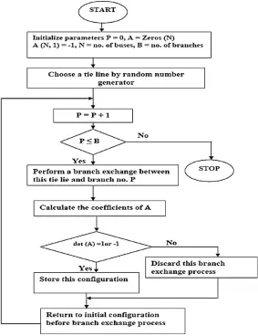
In this section a new algorithm based on the bus incidence matrix A is proposed for checking the radiality of trial solutions. The flow chart of the algorithm is shown in Fig. 1. A graph may be described in terms of a connection or incidence matrix. Of particular interest is the branch-to-node incidence matrix A, which has one row for each branch and one column for each node with an entry axy in row x and column y according to the following rules:

axy= 0 if branch x is not connected to node y (4) axy= 1 if branch x is directed away from node y (5) axy= -1 if branch x is directed toward node y (6)

to be chosen. The column corresponding to the reference node is omitted from A and the resultant matrix is denoted by

A. If the number of branches is equal to the number of nodes then, applying the previous rules a square branch-to-node matrix is obtained. The A matrix has the row–column dimension B × N for any net-work with B branches and N nodes excluding the reference node. By assuming, that there is a branch between this reference node and the root of the network; this will lead to a square matrix if the initial structure of the network is radial. The proposed method is based on the value of the determinant of A. It is found that, if the determinant of A is equal to 1 or −1, then the system is

radial. Else if the determinant of A is equal to zero, means either the system is not a radial or a group of loads are disconnected from the service.

It has the following advantages, they are • It reduces the computation time.

• It restricts each trial solution to be radial network in distribution network reconfiguration.

•

IV. OVERVIEW OF THE DISCRETE PARTICLE SWARM OPTIMIZATION ALGORITHM (TACPSO)

The PSO algorithm is developed by simulating human social behavior and individuals of a swarm. PSO has roots in two main component methodologies. It has been noticed that members within a group seem to share information among themselves-a fact that leads to increased efficiency of the group. The PSO algorithm searches in parallel using a group of individuals similar to other artificial intelligence (AI)-based heuristic optimization techniques. TACPSO is similar to PSO, the particle position is rounded to the nearest discrete value satisfying the position constraints. The TACPSO algorithm searches in parallel using number of individuals. An individual in a swarm approaches the optimum through its present velocity, previous experience, and the experience of its neighbors. In a search space, the position and velocity of an individual are represented as the vectors Xi=(Xi1,Xi2,….Xin) and Vi=(Vi1,Vi2,….Vin). Let Pbest=(Xi1Pbest, Xi2Pbest ,….. Xin Pbest) and Gbesti=(Xi1Gbest, Xi2Gbest ,….. Xin Gbest) respectively, be the best position of and individual and the best position of its neighbors. The updated velocity of an individual is modified under the following equation in the TACPSO algorithm.

Vik+1=W(Vik+C1rand1*(Pbestik-Xik)+C2rand2*(Gbestik-Xik)) (7)

Where C1 and C2 are positive constants, called cognitive and social parameters, respectively, And both are equal to two in general cases; W is the inertia weight factor (a large weight factor facilitates a global search, while a Small inertia weight facilitates a local search; in general, the inertia weight starting at 0.9, linearly decreasing to 0.2 during a run, is adopted to give TACPSO a better Performance);

Vik is the velocity of individual i at iteration k; rand1 and rand2 are random numbers between [0,1]; Xik is the position of individual i at iteration k;

Pbestik is the best position of individual i up to iteration k; and Gbestik is the best position of the group up to iteration k.

Each individual moves from the current position to the next one by using the modified velocity equation (Eq. (7)) in Eq. (8),

Xik+1=round(Xik+Vik+1) (8)

The process of the TACPSO algorithm can be summarized as follows: Step 1: Randomly initialize the group while satisfying

constraints.

Step 2: Velocity and position updates while satisfying constraints.

Step 3: Update of Pbest and Gbest.

Step 4: Go to Step 2 until satisfying stopping criteria. Step 5: Display the results of global best values (Gbest).

Initialization and structure of Individuals

Fig2. Composition of an individual

Fig3. Adjustment strategy for an individual position within a boundary

As shown in Figure 3, the position of the individual at iteration 0 can be represented as the vector of Xi0=(Ti10,…..Tin0), where n is the number of tie switches. The velocity of an individual i (i.e., Vi0=(Vi10,….Vin0). The velocity corresponds to the tie switch update quantity, selected randomly, covering all possible values for tie switches. The following procedure is suggested for any individual in a group:

Step 1: Set j = 1.

Step 2: Select a tie switch from loop j at random.

Step 3: If j = n, then go to Step 4; otherwise j = j + 1 and go to Step 2.

Step4: Stop the initialization process

After creating the initial position of each individual is also created at random.

Velocity Update To modify the position of each individual, it is necessary to calculate the velocity of each individual in the next stage. In this velocity updating process, the values of parameters k, C1, and C2 should be determined in advance. The values of C1 and C2 are considered equal, which implies the same weights are Given between Pbest and Gbest in the evolution processes. The velocity of each particle in the next stage can be updated by using Eq. (7).

Position Modification. The position of each individual is modified by Eq. (8). The resulting position of an individual is not always guaranteed to satisfy the inequality constraints due to over/under velocity.

If any element of an individual violates its boundary condition due to over/under speed, then the position of the individual is fixed to its maximum/minimum operating point. Therefore this can be formulated as

Tijk+1= Tijk+1+Vijk+1 if Tij,min<=( Tijk+1+ Vijk+1)<=Tijmax Tij,min if Tijk+1< Vijk+1< Tij,min

Where Tijk+1 represents the position of the particle, and Tij,min and Tij,max are the boundary values. If the value (Tijk+1= Tijk + Vijk+1) crosses the boundary, then it is set to boundary value. The aforementioned method always produces the position of each individual, satisfying the boundary condition of tie switch position for each loop.

Update of Pbest and Gbest. The Pbest of each individual i at iteration k +1 is Updated as follows Pbestik+1= Xik+1 if TCik+1<TCik

Pbestik+1= Pbestik+1 if TCik+1>TCik Gbestik+1= best(Pbestik+1)

Where TCi , at the position of each individual i, the objective function, is evaluated . Gbest at Iteration k +1 is set as the best evaluated position among Pbestik+1

Stopping Criteria, The TACPSO is terminated if the iteration approaches the predefined no of Maximum iteration.

Parameter selection There exist several parameters to be determined for the Implementation of PSO. In this article, these parameters have been determined through the experiments for the 16-node radial distribution system for loss reduction and the 69-node system for load balancing. The procedures and strategies are adopted as follows:

1) The values of C1 and C2 have the same value, which implies the same weights are given between Pbest and Gbest in the evolution processes.

2) Numbers of particles (10–50) are usually sufficient.

3) Usually C1+C2 = 4, with no good reason other than empiricism (the value taken is solely based on experience).

Repair algorithm

After updating the position of each particle, a position check is carried out to make sure that none of the particles have flown out of the search space bounds. That is all the generated solutions are feasible. If a violation is detected then apply repair algorithm is used to force the violated particle to return to the feasible region as follows:If position of particle (pos(j)) is greater than the maximum position (mp), then pos(j)=mp else if pos(j) is less than one, then pos(j)=1 else end.

V. SOLUTION MECHANISM

The network reconfiguration problem is equivalent to the problem of finding an optimal radial configuration such that the loss is minimized. In this section, the TACPSO algorithm is adapted to solve the network reconfiguration problem. Detailed discussions of each step in implementing the TACPSO are as in the following sections.

Step1:- For each particle, the position and velocity vectors will be randomly initialized with same size.

Step2:- check the network radiality using radiality algorithm this is explained in section III.

Step3:- Measure the fitness (power loss) of

each particle(pbest), the position and store the particle with the best fitness (gbest) value by running the load flow program based on forward sweep method. Step4:- Update velocity and position of each particle according to Eqs. (7) and (8)

Step5:- perform violation check. If violation is detected then apply repair algorithm explained in section IV. Step6:- Repeat steps 2-5 until a stopping a criterion is satisfied.

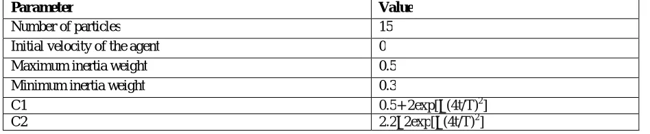
The system load is assumed to be constant and Sbase = 100MVA and Vbase = 12.66KV. The line and load data details can be referred in [5]. The total load on the system is 3715kW and 2300kVAr. The minimum and maximum voltages are set at 0.95 and 1.05p.u.respectively. All calculations for this method are carried out in the per-unit. A computer program is developed to implement the proposed TACPSO algorithm using MATLAB6.5. The TACPSO parameter used during the simulation for the reconfiguration problem is summarized in Table 1.

Fig 4. Initial configuration of the 33 bus distribution system

Table1:- TACPSO parameters used during the simulation

VI. RESULTS AND DISCUSSION

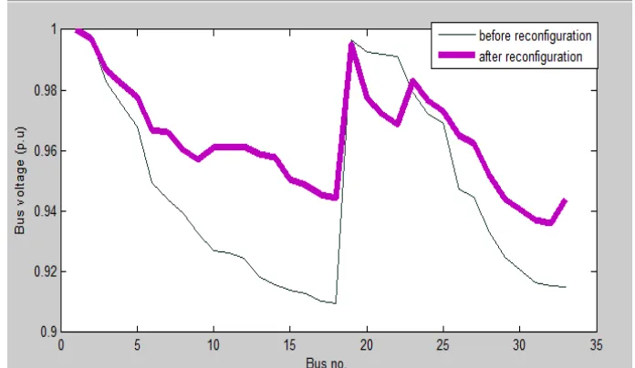
The proposed method is applied to the IEEE 33 bus system to solve the reconfiguration problem using Optimal and Population based proposed method [6,7]. Under base case condition the real power loss is 202.86kW. The lower and upper bounds of the nodal voltage magnitude is Vmax=1p.u and Vmin=0.9097p.u From the table 2. Simulation results show that the power loss after reconfiguration is 139.68kW which is reduced by 31.15% of its initial value. Fig 5. Shows the best moves recorded during the search process, after 10 iteration system leads to power loss reduction (out of 100). The obtained results using the proposed TACPSO algorithm have been reached after 50 trails.

From Fig 6. The voltage profile has been improved by TACPSO algorithm. The minimum bus voltage is 0.9097 under base case and it is raised to 0.9258 after reconfiguration.

Parameter Value

Number of particles 15 Initial velocity of the agent 0 Maximum inertia weight 0.5 Minimum inertia weight 0.3

C1 0.5+ 2exp[−(4t/T)2]

Fig 5. The best moves recorded during the search process for IEEE 33 bus system using TACPSO algorithm

Table 2. Result of 33 bus system using the TACPSO algorithm

Table 3. Objective function statistics for IEEE -33 bus System using the TACPSO algorithm

VII. CONCLUSION

This paper proposed the TACPSO algorithm to solve the optimal reconfiguration problem. The advantage of TACPSO over other method is simplicity. The results obtained during the simulation shows that the TACPSO algorithm is capable of finding the optimal solution. The main objective of this paper is to reduce the real power loss and also improve the voltage profile the bus. A 33-bus distribution system is used to demonstrate the effectiveness of the proposed technique. TACPSO showed the tremendous improvement in term of processing time, number of iterations to reach the optimal value of power losses. The simulation result indicated that the optimal on/off patterns of the tie line can be identified which give the minimum power loss while keeping bus voltage magnitudes within the acceptable limits. Based on these reasons, it is strongly expected that TACPSO is capable of solving large-scale problems arose in network reconfiguration as compared to the existing methods.

REFERENCES

[1] S.Civanlar, J.J. Grainger, H. Yin, S.S.H. Lee, “Distribution feeder reconfiguration for loss reduction”, IEEE Trans. Power Del. 3 (3) (1988) 1217–1223.

[2] X. Jin, J. Zhao, Y. Sun, K. Li, B. Zhang, “Distribution Network Reconfiguration for Load Balancing using Binary Particle Swarm Optimization”, International Conference on Power System Technology, vol. 1, no. 1, Nov. 2004, pp. 507-510

[3] Zhou, Q.; Shirmohammadi, D. and Liu, W.-H. E., “Distribution Feeder Reconfiguration for Operation Cost Reduction”, IEEE Transactions on Power Systems, Vol. 12, No. 2, May 1997, pp. 730-735

[4] T.Ziyu, Z.Dingxue,”A modified particle swarm optimization with an adaptive acceleration coefficient”,Asia-Pacific Conference on Information Processing, Shenzhen, 2009, pp. 330–332.

[5] Smarajit Ghosh, Karma Sonam Sherpa, “An Efficient Method for Load Flow Solution of Radial Distribution Networks”, World Academy of Science, Engineering and Technology, International Journal of Electrical, Computer, Electronics and Communication Engineering Vol:2 No:9, 2008.

[6] Seyed Abbas Taher, Mohammad Hossein Karimi, “ Optimal reconfiguration and DG allocation in balanced and unbalanced distribution system”, Ain Shams Engineering Journa (2014) 5, 735-749.

[7] A.Y. Abdelaziz *, F.M. Mohammed, S.F. Mekhamer, M.A.L. Badr, “Distribution Systems Reconfiguration using a modified particle swarm optimization algorithm”, Electrical Power system research 79(2009)1521-1530.

[8] Yuan-kang Wu, Lee Ching-Yin,Liu Le chang, Tsai Shao – Hong , “Study of reconfiguration for the Distribution system with distributed generators ”, IEEE Trans Power Delivery 2010, 25(3): 1678-85.

[9] Srinivasa Rao R, Narasimham SV, Ramalinga Raju M, Srinivasa Rao A “Optimal network reconfiguration system using harmony search algorithm”, IEEE Trans Power Syst 2011; 26(3),1080-8.

System Power loss Maximum and Minimum

Voltage limits (p.u) Optimal configuration

Before reconfiguration 202.86 kW Vmax=1, Vmin=0.9097 33,34,35,36,37 Ant colony algorithm [8] 142.68kW Vmax=1, Vmin=0.9320 7,10,14,36,37 Harmony search algorithm [9] 139.98kW Vmax=1, Vmin=0.9404 7,9,14,28,32

Proposed method (TACPSO) 138.53kW Vmax=1, Vmin=0.9358 7,9,14,28,36

Best objective function Average objective function Worst objective function