Simulation of Nondifferentiable Models for Groundwater Flow and
Transport
∗C. T. KelleyaK. R. Fowlerb C. E. Keesa
aDepartment of Mathematics and Center for Research in Scientific Computation
North Carolina State University, Box 8205, Raleigh, NC, 27695-8205, USA.
bDepartment of Mathematics and Computer Science Clarkson University,Potsdam, NY
13699-5815, USA
Non-Lipschitz continuous nonlinearities arise frequently in models for groundwater flow and species transport. The van Genuchten and Mualem PSK relations for unsaturated flow and the Freundlich equilibrium expressions in reactive transport are examples. Nu-merical methods such as nonlinear solvers based on Newton’s method, error estimators for differential equations, and stepsize and order control methods for temporal integra-tion, are designed for differentiable problems and may fail when applied to nonsmooth nonlinear problems.
In this paper we consider two approaches to this problem: (1) adding new equations to smooth the nonlinearity and (2) approximating the nonlinearity with a smoother function, such as a spline. In both cases, we replace the non-Lipschitz continuous functions with Lipschitz continuous, but sometimes non-differentiable, nonlinearities. The mathematical properties of Lipschitz continuous nonlinear equations enable standard solvers to work well. We will describe some recent theoretical advances that explain this success and use those results to justify a stepsize and error control strategy for temporal integration. We illustrate the results with two computational examples.
1. INTRODUCTION
Nonsmooth, even non-Lipschitz continuous, constitutive laws are not uncommon in models for groundwater flow and transport. In this paper we consider two example prob-lems with nonsmooth nonlinearities and show how the nonsmoothness can be reduced to a Lipschitz continuous, but non-differentiable, nonlinearity. We will then discuss some theoretical results from [1, 2] on convergence of nonlinear solvers. We will apply those results in § 2 to analyze a first-order integration scheme that incorporates step size and error control.
∗This research was partially supported by National Science Foundation grants 0070641k,
1.1. Richards’ Equation
Richards’ equation (RE) is a simple model of flow in the unsaturated zone [3]. In three space dimensions, letting z be the vertical direction and∇the spatial gradient operator, the pressure head form of RE is
SsSa(ψ)
∂ψ ∂t +η
∂Sa(ψ)
∂t =∇ ·[K(ψ)∇(z+ψ)] (1)
In (1),ψis pressure head, Ssis the specific storage,Sa(ψ) is the aqueous phase saturation,
ηis the porosity, andK(ψ) is the hydraulic conductivity. We will assume that appropriate initial and boundary conditions have been imposed.
In this paper we model saturation with the van Genuchten and Mualem formulae, [4,5],
Sa(ψ) =
(
Sr+ [1+((1α−|ψS|r))n]m, ψ <0
1, ψ ≥0, (2)
K(ψ) =
(
Ks[1−(α|ψ|)
n−1[1+(α|ψ|)n]−m]2
[1+(α|ψ|)n]m/2 , ψ <0
Ks, ψ ≥0
. (3)
In (2) and (3),Sr is the residual saturation,n is an experimentally determined measure
of pore size uniformity, m = 1−1/n, α is an experimentally determined coefficient that is related to the mean pore size, and Ks is the water-saturated hydraulic conductivity.
One can see from (3) that the nonlinearity K is not Lipschitz continuous, much less differentiable, at ψ = 0, if 1 < n < 2. Values of n in this range are physically realistic and solvers must be prepared to deal with nonsmooth nonlinearities.
A common way of dealing with both the nonsmoothness and the cost of the evaluation of the nonlinearity is to approximate the nonlinearity with a spline [2, 6–8]. The simplest such spline, a piecewise linear spline, has been used in practice [7] and found to be effective both computationally and mathematically [1, 2], even though Taylor’s theorem, upon which both Newton’s method and stepsize and error control are based, does not hold.
1.2. Reactive Transport
We consider transport of a reactive solute in porous media using a mass conservative model. We use a formulation that has been studied recently in the context of fully coupled numerical solution techniques for reactive transport problems [9]. The solute reacts with the solid phase, and the reaction rate is assumed to be very fast relative to the transport velocity; more precisely, we assume that the solute in the aqueous phase is in local equilibrium with the solid phase. Furthermore, this solid phase equilibrium concentration is described by the commonly used Freundlich isotherm.
Csθ
ρb
= max(KCr,0) (4)
whereCsis the equilibrium concentration in the solid phase, C is the equilibrium
concen-tration in the aqueous phase,K is the Freundlich coefficient,ris the Freundlich exponent,
ρb is the bulk density of the solid phase, and θ is the porosity. We are interested in the
solute through the porous media can be modeled by combining the Freundlich isotherm with the standard transport equation in porous media [9].
(C+ρb
θ max(KC
r,0))
t+∇ ·[Cv−D∇C] = 0
where v is the mean pore velocity D is the hydrodynamic dispersion tensor.
Numerical solutions of this formulation of the model have not been studied extensively in the non-Lipschitz case, to our knowledge. The approach used to resolve nonlinearities in [9] was to use the auxiliary “fast mass” variable
m=C+ρb
θ max(KC
r,0) (5)
as the primary solution variable. The nonlinear relationC(m) that this approach requires when m >0 was calculated at each outer iteration by finding the root of
f(C) = log(m)−log(C+ρb
θ KC
r)
It is not clear what iterative methods was used to solve this local problem in [9] but they claimed convergence was very fast. Both Picard and Newton outer iterations were tested with this approach and found to be efficient. Furthermore, the formulation above was significantly more robust and efficient than non-conservative formulations of the model.
We view the approach of [9] as a differential algebraic equation (DAE) model. The differential equation is
mt+∇ ·[Cv−D∇C] = 0. (6)
In this paper we reformulate the algebraic constraint as
θmax(m−C,0)
ρbK
!1/r
−C = 0. (7)
Equation (7) is a differentiable, but not Lipschitz continuously differentiable, reformula-tion of (5). A related approach to non-Lipschitz reacreformula-tions has been discussed in [1,10–12].
2. Step size and Error Control
In both of the examples above, we transform a non-Lipschitz nonlinearity to a more tractable Lipschitz continuous or even smooth nonlinearity. Doing this can result in better performance from the nonlinear solver, better robustness, and improved error estimates [1, 2, 6, 8].
original nonlinearity and its smoothed approximation are close, so differentiation must be done carefully if the solver is to succeed [6].
In this paper we assume that the nonlinearity has been smoothed to be Lipschitz continuous, but not necessarily differentiable. In this case nonsmooth analysis [1, 2] can be used to show that Newton’s method, even with a finite-difference Jacobian, will work well to solve the corrector equation in an implicit integration. These results imply that a error control scheme based on comparison of a linear predictor with an implicit Euler step should be reliable, because the nonlinear solver needed to compute the Euler step is reliable. We can therefore quantify how a first order error control method works in the presence of a nonsmooth nonlinearity.
In this section we analyze a model problem based on a system of ordinary differential equations. Discretizing a PDE with the method of lines produces just such a system. In § 3, however, the equations are DAEs, and the analysis predicts the performance of the integrator in that more complex setting.
Consider an initial value problem for a system of ordinary differential equations
y0 =f(y), y(0) =y0, (8)
where f is Lipschitz continuous. Assume that a solution y exists for 0 ≤ t ≤ T. The continuity of f implies thaty is Lipschitz continuously differentiable, but not necessarily twice differentiable.
We begin the design of a first-order stepsize and error control scheme as one would in smooth case. Leth >0 be given and t∈[0, T −h] Clearly
y(t+h) =y(t) +y0(t+h)h+h
Z 1
0 y
0(t+αh)−y0(t+h)dα,
and so the local truncation error in the implicit Euler method is
Ee =h
Z 1
0 y
0(t+αh)−y0(t+h)dα=O(h2).
Error estimation uses previously computed results at t and t−¯h. One compares the implicit Euler result to a linear predictor
yp =y(t) +h
y(t)−y(t−h¯) ¯
h
!
.
The error in the predictor is
Ep =h
Z 1
0 y
0(t+αh)−y0(t−α¯h)dα
Now, sincey0 =f(y), we have
y0(t+αh)−y0(t+h) =f(y(t+αh))−f(y(t+h)).
integral norm (in space), it is reasonable to expect the Lipschitz constant of f(y(t)) to vary slowly as a function of t.
If we assume that f is a local function of y, as it is in the case of the spatial deriva-tive term in Richards’ equation and the scalar constituderiva-tive law in the reacderiva-tive transport problem, we may assume that
kf(y(t+αh))−f(y(t+h))k ≈L(y0(t))|1−α|h
where L(y0(t)) is the local Lipschitz constant for y0(t) =f(y(t)), which we assume varies slowly in t.
If these assumptions are valid, then
kEek ≈L(y0(t))h2/2 and kye−ypk=≈L(y0(t))(h2−h¯h/2). (9)
Step size and error control is based on (9).
In the integration, given implicit Euler steps{yj}nj=0−1 and steps {hj}nj=0 we computeyn
by solving
yn=yn−1+hnf(yn).
We then compareyn to the predicted value
yp
n=yn−1+hn
yn−1−yn−2
hn−1
and use (9) to estimate L(y0(t
n)) by
Ln=
2kyn−ynpk
|2h2
n−hnhn−1|
. (10)
We then compute hn+1 so that the estimated local truncation error
Lnh2n+1/2≤.9τ, (11)
where τ is the tolerance for the integration and the safety factor of .9 is the suggestion from [17].
3. Numerical Results
We present two sets of calculations, one for Richards’ equation and the other for reactive transport. In each case we compare Ln, the estimated Lipschitz constant of y0, with the
actual value of
L(yn0) = kf(y(tn))−f(y(tn−1))k (tn−tn−1)
(12)
using the L2 norm. We consider mesh sizes of ∆z = 1/100,1/200,1/400,and 1/800. For
3.1. Richards’ Equation
To test the first order step-size and error control scheme for Richards’ equation, we simulate flow through homogeneous, 1-D 10m long columns of soil. The simulator uses piecewise linear finite elements in space and backward Euler in time with Newton’s method as the nonlinear solver. We consider two media, clay and silt, which have a value of 1< n <2,making the nonlinearities in (2) and (3) non-Lipschitz. The media begins fully unsaturated and we set the pressure head at the top of the domain so that infiltration begins at the start of the simulation. Infiltration problems of this type are known to be numerically challenging and would require a very small fixed time step in the absence of error control [6, 18].
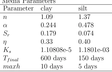
The physical data for these problems is given in Table 1. We sampled 5000 points for the spline approximations to the nonlinearities in (2) and (3) on the interval−15≤ψ ≤0
Table 1
Media Parameters
Parameter clay silt
n 1.09 1.37
α 0.244 0.478
Sr 0.179 0.074
η 0.33 0.40
Ks 1.10808e-5 1.1801e-03
Tf inal 600 days 150 days
maxh 10 days 5 days
For the results in this section we used τ = 10−2, and an initial time step of 10−9.
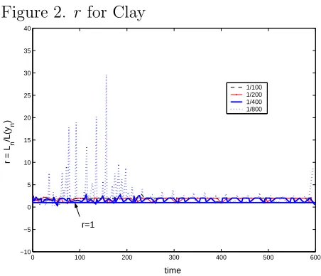
Figures 1 and 2 show r as a function of time
Figure 1. r for Silt
0 50 100 150
−2 −1 0 1 2 3 4 5 6
time
r = L
n
/L(y
n
)
1/100 1/200 1/400 1/800
Figure 2. r for Clay
0 100 200 300 400 500 600
−10 −5 0 5 10 15 20 25 30 35 40
time
r = L
n
/L(y
n
)
1/100 1/200 1/400 1/800
r=1
The estimates of the Lipschitz constant were within a factor of two or three for most of the integrations. The errors were overestimates in most cases. The minimum underes-timate was a factor of two for all but the 1/200 grid, where the minimum underesunderes-timate was a factor of three for the clay problem.
3.2. Reactive Transport
The semi-discrete equations for the reactive transport problem are a DAE of the form
M0 = F(C) (13)
G(C,M) = 0 (14)
The analysis and formulas in the previous section require some alterations because they were derived for and ODE. For step size adaption we use the estimate
Ln=
2kMn−Mpnk
|2h2
n−hnhn−1|
(15) and we estimate the Lipschitz constant of M0 using
L= kF(C(tn))−F(C(tn−1))k (tn−tn−1)
(16) Since ∂G
∂C is invertible for all C (it is a diagonal matrix with non-zero diagonals), we
have by the implicit function theorem that
C= ¯G(M). (17)
The DAE is then locally equivalent to the ODE
M0 =F( ¯G(M(t))), (18)
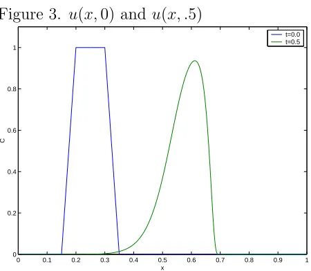
For the reactive transport model we consider a 1D test problem on [0,1] with u(0, t) =
u(1, t) = 0 and initial data given by
u(x,0) =
0 x≤0.2−0.05 1−(0.2−x)/0.05 0.2−0.05< x <0.2
1 0.2≤x≤0.3
1 + (0.3−x)/0.05 0.3< x <0.3 + 0.05 0 x≥0.3 + 0.05
The parameters for the test problem are given in table 2 [9]. We discretized the equa-tion using backward Euler in time, upwind finite differences for the advecequa-tion term, and central differences for the diffusion term. Newton’s method was used to solve the resulting nonlinear systems to a relative residual tolerance of 10−6. Jacobians were inverted using
an LU factorization. We integrated to t = 0.5. The initial conditions and solution are given in figure 3. The ratio of the Lipschitz constants is given in figure 4. The variation on the ratio at the beginning and end of the integration is due to the rapid variation in step-size from the initial step size and for the final step to t= 0.5.
Table 2
Reactive Transport Parameters
D 4.0e-4 v 1.0
r 0.7 K 0.126
ρb 1.59 θ 0.4
Figure 3. u(x,0) andu(x, .5)
0 0.1 0.2 0.3 0.4 0.5 0.6 0.7 0.8 0.9 1
0 0.2 0.4 0.6 0.8 1
x
C
Figure 4. r for Reactive Transport: smooth formulation
0 0.1 0.2 0.3 0.4 0.5
0.5 1 1.5 2 2.5 3
time
r=L
n
/L(y
n
)
1/100 1/200 1/400 1/800
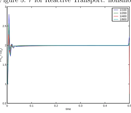
We also tested approximating the original non-Lipschitz formulation by using a piece-wise linear spline of the Freundlich isotherm in a neighborhood of the non-Lipschitz point. Instead of (7) we used
m=C+
ρbK
θ C
r C ≥10−4
ρbK
θ 104(1−r)C 0≤C <10−4
0 C <0
(19)
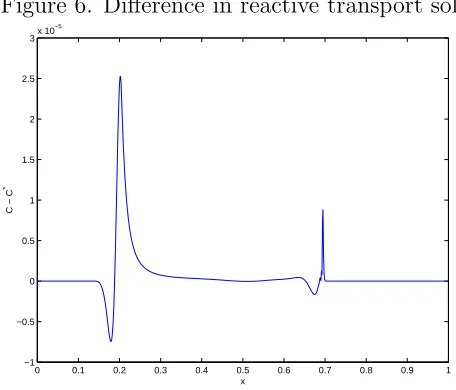
Both the performance of the integrator and the solution were virtually identical. The ratios are plotted in Figure 5 and the differences in the solutions in Figure 6.
Figure 5. r for Reactive Transport: nonsmooth formulation
0 0.1 0.2 0.3 0.4 0.5
0.5 1 1.5 2 2.5 3
time
r=L
n
/ L(y
n
)
Figure 6. Difference in reactive transport solutions
0 0.1 0.2 0.3 0.4 0.5 0.6 0.7 0.8 0.9 1
−1 −0.5 0 0.5 1 1.5 2 2.5
3x 10 −5
x
C − C
*
4. Conclusions
We have show that first order error estimation and control works correctly for certain Lipschitz continuous nonlinearities that arise in the simulation of subsurface flow and species transport. We have analyzed the ODE case, and performed computations for the more general DAE case. Our computions illustrate the potential to make reactive transport calculations more robust by the kind of variable transformation that was done in [1, 9, 10, 19].
Acknowledgements
The authors are grateful to Matthew Farthing for providing the reactive transport test problem and its dense grid solution.
REFERENCES
1. K. R. Fowler and C. T. Kelley. Pseudo-transient continuation for nonsmooth nonlinear equations. Technical Report CRSC-TR03-29, North Carolina State University, Center for Research in Scientific Computation, July, 2003.
2. K. R. Kavanagh. Nonsmooth Nonlinearities in Applications from Hydrology. PhD thesis, North Carolina State University, Raleigh, North Carolina, 2003.
3. L. A. Richards. Capillary conduction of liquids through porous media. Physics, 1:318–333, 1931.
4. M. T. van Genuchten. Predicting the hydraulic conductivity of unsaturated soils. Soil Science Society of America Journal, 44:892–898, 1980.
5. Y. Mualem. A new model for predicting the hydraulic conductivity of unsaturated porous media. Water Resources Research, 12(3):513–522, 1976.
of Richards’ equation for non-uniform porous media. Water Resources Research, 34:2599–2610, 1998.
7. Kimberlie Staheli, Joseph H. Schmidt, and Spencer Swift. Guidelines for Solving Groundwater Problems with ADH, January 1998.
8. K. R. Kavanagh, C. T. Kelley, R. C. Berger, J. P. Hallberg, and Stacy E. Howing-ton. Nonsmooth nonlinearities and temporal integration of Richards’ equation. In S. Majid Hassanizadeh, Ruud J. Schotting, W. G. Gray, and G. F. Pinder, editors,
Computational Methods in Water Resources XIV, Vol. 2, pages 947–954, Amsterdam, 2002. Elsevier.
9. J. F. Kanney, C. T. Miller, and D. A. Barry. Comparison of fully coupled approaches for approximating nonlinear transport and reaction problems. Advances in Water Resources, 26(4):353–372, APR 2003.
10. X. Chen. A superlinearly and globally convergent method for reaction and diffusion problems with a non-lipschitzian operator. Computing [suppl], pages 79–90, 2001. 11. A. K. Aziz, A. B. Stephens, and M. Suri. Numerical methods for reaction-diffusion
problems with non-differentiable kinetics. Numer. Math., 53:1–11, 1988.
12. J. W. Barrett and R. M. Shanahan. Finite element approximation of a model reaction - diffusion problem with a non-Lipschitzian nonlinearity. Numer. Math., 59:217–242, 1991.
13. C. T. Kelley. Iterative Methods for Linear and Nonlinear Equations. Number 16 in Frontiers in Applied Mathematics. SIAM, Philadelphia, 1995.
14. C. T. Kelley. Solving Nonlinear Equations with Newton’s Method. Number 1 in Fundamentals of Algorithms. SIAM, Philadelphia, 2003.
15. J. M. Ortega and W. C. Rheinboldt. Iterative Solution of Nonlinear Equations in Several Variables. Academic Press, New York, 1970.
16. J. E. Dennis and R. B. Schnabel. Numerical Methods for Unconstrained Optimization and Nonlinear Equations. Number 16 in Classics in Applied Mathematics. SIAM, Philadelphia, 1996.
17. U. M. Ascher and L. R. Petzold. Computer Methods for Ordinary Differential Equa-tions and Differential Algebraic EquaEqua-tions. SIAM, Philadelphia, 1998.
18. M. D. Tocci, C. T. Kelley, and C. T. Miller. Accurate and economical solution of the pressure head form of Richards’ equation by the method of lines. Advances in Water Resources, 20:1–14, 1997.