Simulation Algorithms for Continuous Time Markov
Chain Models
H.T. Banks1, Anna Broido2, Brandi Canter3, Kaitlyn Gayvert4, Shuhua Hu1
, Michele Joyner3
, Kathryn Link5 1
Center for Research in Scientific Computation Center for Quantitative Sciences in Biomedicine
North Carolina State University Raleigh, NC 27695-8212 USA
2
Department of Mathematics Boston College
Chestnut Hill, MA 02467-3806 USA
3
Department of Mathematics and Statistics East Tennessee State University Johnson City, TN 37614-70663 USA
4
Department of Mathematics State University of New York at Geneseo
Geneseo, NY 14454 USA
5
Department of Mathematics Bryn Mawr College Bryn Mawr, PA 19010-2899 USA
December 14, 2011
Abstract
Continuous time Markov chains are often used in the literature to model the dy-namics of a system with low species count and uncertainty in transitions. In this pa-per, we investigate three particular algorithms that can be used to numerically simu-late continuous time Markov chain models (a stochastic simulation algorithm, explicit and implicit tau-leaping algorithms). To compare these methods, we used them to an-alyze two stochastic infection models with different level of complexity. One of these models describes the dynamics of Vancomycin-Resistant Enterococcus (VRE) infec-tion in a hospital, and the other is for the early infecinfec-tion of Human Immunodeficiency Virus (HIV) within a host. The relative efficiency of each algorithm is determined based on computational time and degree of precision required. The numerical results suggest that all three algorithms have similar computational efficiency for the VRE model due to the low number of species and small number of transitions. However, we found that with the larger and more complex HIV model, implementation and modification of tau-Leaping methods are preferred.
1
Introduction
Deterministic approaches involving ordinary differential equations to approximate large number discrete populations with a continuum, though widely used, have proven less useful when applied (often with little or no justification!) to small sample sizes. To ad-dress this issue, continuous time Markov chain (CTMC) models are often used when dealing with low species or population counts. There are a variety of stochastic algo-rithms that can be employed to simulate CTMC models. However, it appears that none of these algorithms is universally efficient in many problems of interest.
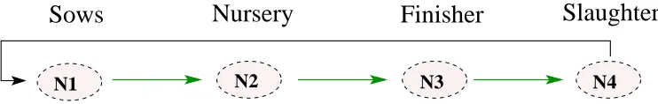
There are a plethora of applications in which the questions we investigate here arise. In addition to the infection models we use for illustration, similar stochastic models arise in just-in-time production networks, manufacturing and delivery, logistic/supply chains, and multi-scale (large/small) population models as well as network models in commu-nications and security. A typical example is the agricultural (pork) production system investigated in [2]. There a stochastic transport model was used to study the impact of disturbances (introduction of diseases and other disruptions in the network) in produc-tion systens such as that depicted in Figure 1.
Slaughter
Finisher
Nursery
Sows
N4 N3
N1 N2
Figure 1: Aggregated agricultural network model.
The schematic represents a simplified swine production network with four levels of production nodes: (i) growers/sows (N1), (ii) nurseries (N2), (iii) finishers (N3), and (iv) processing plants/slaughterhouses (N4). At the grower or sow farms (N1), new piglets are born and weaned approximately three weeks after birth. The three-week old piglets are moved to nursery farms (N2) to mature for another seven weeks. They are then trans-ferred to the finisher farms (N3) where they grow to full market size. This takes approx-imately twenty weeks. Once they reach market weight, the matured pigs are moved to the processors (slaughterhouses) (N4).
quickly spread throughout the system. Other interruptions occur when nurseries supply-ing farms have nowhere to send animals as they mature if the farms have not cleared their current animals for some reason. This will cause finishers and slaughterhouses to have supply interrupted. Randomness seen in the stochastic network model originates from random movement of discrete “individuals” from node to node. Analysis (see [2]) shows that, due to an averaging effect, these random effects become less important as the sys-tem size (numberN of “individuals”) increases. We observe that an application of such a stochastic transportation model to describe the system behavior should account for size of groups in which pigs are transported between nodes. If thousands of pigs are moved at a time, an appropriate notion of an “individual” in the context of the model might be a thousand pigs. Then treating each group of a thousand animals as unit would lead to a marked increase in magnitude of stochastic fluctuations seen at the “population” level. As a result, scaling in the model may result in vastly different stochastic fluctuations in model simulations. Thus one must exercise care in how data and “units” are formulated in modeling populations.
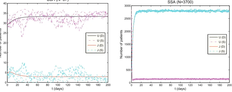
To further illustrate these practical modeling concerns, we consider the results related to our investigations below of Vancomycin-Resistant Enterococcus (VRE) transmission among patients in hospital intensive care units. Figure 2 depicts the results obtained when comparing stochastic model simulations with corresponding deterministic ordi-nary differential equation formulations for the total number of bedsN = 37(left panel) and N = 3700(right panel). The figure reveals that behaviors of the model simulations are quite different when treating one 3700 bed unit as 37 bed units in 100 hospitals if we could argue (not often plausible) that the units are similar in patient and health care worker routines. This offers rather clear warnings for the indiscriminate use of limiting deterministic ordinary differential equations in place of Markov chain models to study small population count systems.
Fundamental to the investigation of such systems is the ability to efficiently simulate the systems in the context of inverse problems, parameter estimation, sensitivity, con-trol, etc. Computational methods abound for the corresponding deterministic limiting (as population size increases) differential equations. While a number of stochastic simu-lation algorithms exist, they are often difficult to use in the contexts mentioned above.
The goal of this paper is to illustrate how widely performances may vary for some stochastic algorithms when compared on two stochastic infection models and to demon-strate how one might perform computational studies to aid in selection of appropriate algorithms. Specifically, we examine three commonly used algorithms: a stochastic simu-lation algorithm (SSA), and explicit and implicit tau-leaping methods. One of the models used to demonstrate the efficiency of these three algorithms describes progression of a Vancomycin-resistant enterococcus (VRE) infection in a hospital unit. The other model describes the dynamics of HIV during the early stage of infection, in which the target cells are still at very high level while the infected cells are at very low level.
tau-0 20 40 60 80 100 120 140 160 180 200
0
5
10 15 20 25 30 35 40
t (d ays ) Nu
m
be
r
o
fp
a
ti
e
n
ts
U (D ) U (S ) J (D ) J (S )
0 20 40 60 80 100 120 140 160 180 200
0
500 1000 1500 2000 2500 3000
t (d ays ) Nu
m
be
r
o
fp
a
tie
n
ts
S S A (N = 3 7 0 0 )
U (D ) U (S ) J (D ) J (S )
Figure 2: Results from VRE model simulations: Graphs in the left column are for un-colonized patients (U) and colonized patients in isolation (J) and N=37 and the ones in right column are for uncolonized patients (U) and colonized patients in isolation (J) and N=3700. The (D) and (S) in the legend denote the solutions obtained with the deter-ministic VRE model and stochastic VRE model introduced below, respectively, where the stochastic results are obtained with the SSA.
leaping algorithms. In Section 3 we apply these three stochastic algorithms to the VRE and HIV models and compare their computational efficiency. We conclude the paper in Section 4 with some summary remarks.
2
Simulation Algorithms
In this section, three computational algorithms for solving stochastic systems will be ex-amined, the stochastic simulation algorithm, the explicit tau-leaping method and the im-plicit tau-leaping method. Outlines for implementing each algorithm will be given along with motivations for the algorithm and discussions about when one might want to use one algorithm over another.
Unless otherwise indicated, a capital letter is used throughout to denote a random variable, a bold capital letter is for a random vector, and their corresponding small letters are for their realizations.
2.1
Stochastic Simulation Algorithm
come in whole numbers as well as the inherent degree of randomness in their dynamical behavior. However, in addition to simulating chemically reacting systems, the Gillespie algorithm has become the method of choice to numerically simulate stochastic models arising in a variety of other biological applications [1, 2, 12, 13, 16, 17].
Two mathematically equivalent procedures were originally proposed by Gillespie, the “Direct method” and the “First Reaction method”. Both procedures are exact procedures rigorously based on the chemical master equation [8]; however, the direct method is the method typically implemented due to its efficiency. Likewise, this is the method em-ployed in this paper. The direct method can be described for a general system by as-suming X = (X1, X2, ..., Xn)T represents the state variables of the system where Xi(t) denotes the number in stateXi at timet(Ximay be the number of patients, cells, species,
etc). Furthermore, it is assumed ltransitions (often referred to as reaction channelsin the biochemistry literature) are possible with associated transition rates (often referred to as propensity functions in the biochemistry literature) represented by λi, i = 1, ..., l. Given
this terminology, the direct method for the Gillespie algorithm can be described by the following procedure:
Step 1. Initialize the state of the systemx0;
Step 2. For the given statexof the system, calculate the transition ratesλi(x),i= 1, ..., l;
Step 3. Calculate the sum of all transition rates,λ=
l
X
i=1
λi(x);
Step 4. Simulate the time,τ, until the next transition by drawing from an exponential dis-tribution with mean1/λ;
Step 5. Simulate the transition type by drawing from the discrete distribution with proba-bility Prob(transition=i) =λi(x)/λ. Generate a random numberr2from a uniform distribution and choose the transition as follows: If0< r2 < λ1(x)/λ, choose transi-tion 1; ifλ1(x)/λ < r2 <(λ1(x) +λ2(x))/λchoose transition 2, and so on;
Step 6. Update the new timet =t+τ and the new system state;
Step 7. Iterate steps 2-6 untilt≥tstop.
2.2
Tau-Leaping Methods
transitions take place during a given subinterval. It is assumed that the value of the leap, τ, is small enough that there is no significant change in the value of the transition rates along the subinterval [t, t+τ]. This condition is known as the leap condition. The tau-leaping method thus has the advantage of simulating many transitions in one leap while not losing significant accuracy, resulting in a speed up in computational time. In this paper, we consider two tau-leaping methods, an explicit and an implicit tau-leaping method.
2.2.1 An Explicit Tau-Leaping Method
The explicit tau-leaping method is based on an explicit formulation for the update in number of speciesXat timet+τ, givenX(t) =x. The basic explicit tau-leaping method approximatesKj, the number of times a transitionj is expected to occur within the time
interval [t, t+τ], by a Poisson random variable Pj(λj(x), τ) with mean (and variance)
λj(x)τ. Once the number of transitions are estimated, the approximate number of species,
known as thetau-leaping approximation, ofXat timet+τ is given by the formula
X(t+τ) =x+
l
X
j=1
Pj(λj(x), τ)vj (2.1)
with vj = (v1j, ..., vnj)T where vij represents the change in state variable Xi caused by
transitionj [6]. However, as mentioned previously, the process for selectingτ is critical in the tau-leaping method. Ifτ is chosen too small, tau-leaping will essentially stop, leading to the standard SSA algorithm; on the other hand, if the value of τ is too large, the leap condition may not be satisfied, possibly causing significant inaccuracies in the simulation. In this paper, we use aτ-selection procedure based on the algorithm in [6]. For alternative procedures for selectingτ, we refer the reader to references [6, 9, 10].
Let ∆Xi =Xi(t+τ)−xi withxibeing theith component ofx, i= 1,2, . . . n, andǫbe
an error control parameter with0< ǫ≪1. In the givenτ-selection procedure,τ is chosen such that
∆Xi ≤max
ǫ
gi
xi,1
, i= 1, ..., n, (2.2)
which evidently requires the relative change inXito be bounded by
ǫ
gi
except thatXiwill
never be required to change by an amount less than 1. The value of gi in (2.2) is chosen
such that the relative changes in all the transition rates will be bounded byǫ.
leap-interval. In some instances, if a population or number of species is small at the be-ginning of the leap-interval, the estimate of the state variable after numerous transitions may result in a negative population. To avoid this situation, Cao, et al. [5, 6] introduced another control parameter,nc, a positive integer (normally set between 2 and 20) which is
used to separate transitions into two classes, critical transitions or noncritical transitions. A transitionj is deemed critical if afternc of these transitions, there is a danger in one of
the state variables involved in the transition reaching zero. An estimate for the maximum number of timesLj,j = 1, ...l that transitionj can occur before reducing one of the state
variables involved in the transition to 0 (or less) is calculated by
Lj = min
{1≤i≤n;νij<0}
xi
|vij|
with the brackets indicating the floor function. If Lj is less than the control parameter
nc, then the reaction is deemed critical. All critical transitions are then restricted to a
single transition during the leap period reducing the probability of a negative population to nearly zero. All the remaining noncritical transitions use the traditional tau-leaping method. The algorithm for the modified explicit tau-leaping method is given below.
Step 1. Given X(t) = x, identify all critical transitions by first estimating the maximum number of times,Lj, that a transition can occur before causing a negative population
where
Lj = min
{1≤i≤n;νij<0}
xi
|vij|
with the brackets indicating the floor function. A transition is considered critical if
Lj < nc. (In our calculations, we setnc =10)
Let
Jcr ={j ∈ {1, ..., l}|jis a critical transition}
and
Jncr ={j ∈ {1, ..., l}|j is a noncritical transition}.
Step 2. Choose a value for the error control parameter ǫ. (In our calculations, we set ǫ = 0.03). Then, compute τ1 so each transition rate λj, j = 1, ..., l is bounded byǫ,
ac-cording to the following definitions:
τ1 = min 1≤i≤n
(
max{ǫxi/gi,1}
|µˆi(x)|
,max{ǫxi/gi,1}
2
ˆ
σ2
i(x)
)
(2.3)
whereµˆi(x) =
X
j∈Jncr
vijλj(x), ˆσi2(x) =
X
j∈Jncr
v2
ijλj(x), andgi as described in the text,
Step 3. Determine whether tau-leaping is appropriate by comparingτ1 to1/λ. Ifτ1 is less than some multiple of1/λ(chosen to be 10 in our calculations), then abandon tau-leaping and execute a set number of single transition SSA steps (chosen to be 100 in our calculations) and return to step 2. Otherwise proceed.
Step 4. Compute the sum of all critical transition rates
λc = X
j∈Jcr
λj(x).
Generate a second candidate time leap, τ2 as a sample of the exponential random variable with mean1/λc
.
Step 5. Letτ = min{τ1, τ2}. Approximate the number of transitions within the time interval,
Kj, as a sample of the Poisson random variable with mean λj(x)τ for allj ∈ Jncr.
For all critical transitions, defineKj as follows:
• Ifτ =τ1, setKj = 0for allj ∈Jcr (no critical transitions occur).
• If τ = τ2, let jc be a sample of the integer random variable with point
proba-bilitiesλj(x)/λc forj ∈ Jcr. SetKjc = 1(jc indicates the only critical transition
which occurs) andKj = 0forj ∈Jcr, j 6=jc(only one critical transition occurs).
Step 6. If there is a negative component inx+X
j
Kjvj, reduceτ1 by half and return to step
3. Otherwise leap by replacing the time,t =t+τ and then update the new system state,
x(t+τ) =x+X
j
Kjvj.
Step 7. Iterate steps 1-6 untilt≥tstop.
2.2.2 An Implicit Tau-Leaping Method
In many applications, such as the HIV model explained in Section 3.2, problems of “stiff-ness” may arise. Rathinam et al. [15] explored the nature of stiffness in discrete stochastic systems and demonstrated that an implicit tau-leaping method (similar to implicit Eu-ler methods for ordinary differential equations) is capable of taking large time steps for stiff, discrete systems, producing accurate results for such systems while significantly re-ducing the computational time when compared to explicit tau-leaping methods [11]. The implicit tau-leaping method replaces the explicit update formula given in equation (2.1) by an implicit tau-leaping formula given by
X(t+τ) =x+
l
X
j=1
Note that the above formula typically gives a non-integer vector forX(t+τ). To overcome this difficulty, Rathinam et al. [15] proposed a two-stage process given by
e
X=x+
l
X
j=1
Pj(λj(x), τ)−λj(x)τ+λj(Xe)τ
vj, (2.4)
and
X(t+τ) =x+
l
X
j=1
r
Pj(λj(x), τ)−λj(x)τ +λj(Xe)τ
z
vj, (2.5)
whereJzKdenotes the nearest non-negative integer corresponding to a real numberz. The implicit tau-leaping method does not have a stability limitation as does the ex-plicit tau-leaping (i.e., the relative changes in all the transition rates are bounded by ǫ) due to the implicitness of the scheme. In [7] the stepsize for the stiff system is chosen to bound the relative changes of those transition rates resulting from the non-equilibrium reactions byǫ, thus, a larger stepsize is allowed. However, as remarked by the authors in [7], it is generally difficult to determine whether or not a reaction is in partial equilib-rium, and the partial equilibrium condition is only formulated in [7] for those reversible reaction pairs for some biochemical systems. To overcome this difficulty, in this paper we use (2.3) to choose τ1 for the implicit tau-leaping method but with a largerǫ to allow a possible large time stepsize.
To avoid the possibility of negative populations (i.e., to ensure (2.4) has non-negative solution), the algorithm for implicit tau-leaping is implemented in the same way as that for the explicit tau-leaping method except the update for states (i.e., replace (2.1) by (2.4) and (2.5)).
3
Numerical Examples
In this section, we report on applying the SSA, explicit and implicit tau-leaping algo-rithms to two stochastic infection models in the literature. One is used to describe VRE infection in a hospital. The other describes the early HIV infection within a host. All three algorithms were coded in Matlab, and all the simulation results were run on a linux machine with a 2GHz Intel Xeon Processor with 8GB of RAM total.
The following notation will be used throughout the subsequent discussions: Zn is the set of n-dimensional column vectors with integer components, and ei ∈ Zn is the
ith unit column vector, that is, the ith entry of ei is 1 and all the other entries are zeros,
i= 1,2, . . . , n.
3.1
VRE Model
tau-leaping methods. In this model, the dynamics of VRE infection is modeled as a continu-ous time Markov chain, and a constant population is assumed so that the hospital remains full for all time; that is, the overall admission rate equals the overall discharge rate. LetN
denote the total number of beds available in the hospital, and{XN(t), t ≥0}be a contin-uous time Markov chain withXN = (XN
1 , X
N
2 , X
N
3 )
T
, where the meanings of the random variablesXiN,i= 1,2,3are given in Table 1.
Variables Description
X1N(t) Number of uncolonized patients at timetin a hospital withN beds
X2N(t) Number of VRE colonized patients at timetin a hospital withN beds
X3N(t) Number of VRE colonized patients in isolation at timetin a hospital withN beds Table 1: State variables for the VRE model.
In any small time interval of length ∆t, the process{XN(t), t ≥ 0}jumps from state xN toxN +vj with probabilityλj(xN)∆t+o(∆t), that is,
ProbXN(t+ ∆t) =xN +vj |XN(t) =xN =λj(xN)∆t+o(∆t), j = 1,2, . . . , l, (3.1)
where xN = (xN
1 , x
N
2 , x
N
3 )
T ∈
Z3 , vj ∈ Z3, and λj is the transition rate for transition
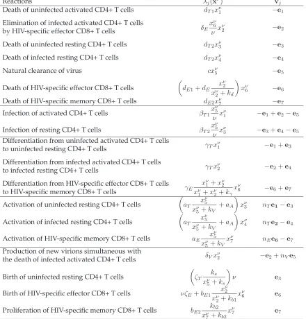
j given in the second column of Table 2 (see [13] for details on the rationale behind in deriving these transition rates). From this table, we see that there are five transition rates
Reactions λj(xN) vj
X1N →X
N
2 mµ1xN1 +βx
N
1 (x
N
2 + (1−γ)x
N
3 ) −e1+e2
X3N →X
N
2 mµ2xN3 e2−e3
X2N →X
N
1 (1−m)µ2xN2 e1−e2
X3N →X
N
1 (1−m)µ2xN3 e1−e3
X2N →X
N
3 αx
N
2 −e2+e3
Table 2: Transition rates λj(xN) as well as the corresponding state changes vj for the
stochastic VRE model.
(i.e.,l = 5), and the corresponding states changesvj are listed in the third column of this table.
3.1.1 Numerical Results
Numerical results were obtained by applying the SSA, explicit tau-leaping and implicit tau-leaping to the stochastic VRE model (3.1) with transition rates given in Table 2. We compare the computational time of the SSA, explicit and implicit tau-leaping methods with different values ofN. All the simulations were run for the time period [0,200] days with parameter values given by
and initial conditions XN(0) = N
29 37,
4 37,
4 37
T
. That is, all the simulations start with
the same initial density
29 37,
4 37,
4 37
T
.
For the tau-leaping methods, the value ofgi is found to begi = 4, i = 1,2,3, and the
value ofǫis set as 0.3 for the implicit tau-leaping. This is chosen based on the simulation results so that the computational time is comparatively short without compromising the accuracy of the solution.
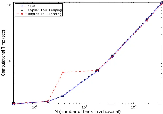
Figure 3 depicts the computational time of each algorithm for an average of five typ-ical simulation runs with N varying from37,185,370,1850,3700,18500,37000. From this
102 103 104
101 102
N (number of beds in a hospital)
Computational Time (sec)
SSA
Explicit Tau−Leaping Implicit Tau−Leaping
Figure 3: Comparison of computational time of different algorithm (SSA, Explicit Tau-Leaping and Implicit Tau-Tau-Leaping) for an average of five typical simulation runs.
figure, we see that the computational time for all the algorithms increases as the value
N increases. This is expected for the SSA as the mean time stepsize for the SSA is the inverse of the sum of all transition rates, which increases asN increases (roughly propor-tional toN2
N continues to increase, we see that the computational times for the implicit tau-leaping are similar to those of the SSA and the explicit tau-leaping methods. This is because the time stepsize becomes significantly higher than the those of these two methods which compensates for the time consuming solving of systems of nonlinear equations. As we can see from (2.3) and the transition rates illustrated in Table 2, ifǫxi/gi >1, then the first
term inside the minimum sign of (2.3) is roughly proportional to 1/N while the second term is roughly proportional to 1. The simulation results show that the first term inside of the minimum sign of (2.3) is smaller than the second term whenN increases to 1850 and above. Hence, the time stepsize for the implicit tau-leaping method decreases as N in-creases whenN ≥1850. This implies the computational time for the implicit tau-leaping method increases as N increases. Based on the above discussions, we see that the SSA performs similarly to the tau-leaping methods (and may be slightly better in some cases). Due to its simplicity and accuracy, the SSA is the best choice for this particular problem.
3.2
HIV Model
We adopted the stochastic model developed in [3] for the dynamics of early HIV infec-tion within a host to demonstrate the computainfec-tional efficiency of the SSA, explicit and implicit tau-leaping methods. In this model the dynamics of HIV infection are modeled as a continuous time Markov chain. Let ν denote the volume of blood (unit: µl-blood), and{Xν(t), t ≥ 0}be a pure jump Markov process with Xν = (Xν
1, X
ν
2, . . . , X
ν
7)
T
, where the meanings of random variablesXν
i, i = 1,2, . . . ,7are stated in Table 3. In any small
Variables Description
X1ν(t) number of non-infected activated CD4+ T-cells inν µl-blood at timet
Xν
2(t) number of infected activated CD4+ T-cells inν µl-blood at timet
X3ν(t) number of non-infected resting CD4+ T-cells inν µl-blood at timet
X4ν(t) number of infected resting CD4+ T-cells inν µl-blood at timet
Xν
5(t) number of RNA copies of infectious free virus inν µl-blood at timet
X6ν(t) number of HIV-specific effector CD8+ T-cells inν µl-blood at timet
X7ν(t) number of HIV-specific memory CD8+ T-cells inν µl-blood at timet Table 3: State variables for the stochastic HIV model.
time interval of length∆t, the process {Xν(t), t ≥ 0}jumps from statexν toxν +vj with probabilityλj(xν)∆t+o(∆t). That is,
Prob{Xν(t+ ∆t) =xν +vj |Xν(t) =xν}=λj(xν)∆t+o(∆t), j = 1,2, . . . , l, (3.2)
where xν = (xν
1, x
ν
2, . . . , x
ν
7)
T
Reactions λj(xν) vj Death of uninfected activated CD4+ T cells dT1xν1 −e1
Elimination of infected activated CD4+ T cells
δEx ν 6 ν x
ν
2 −e2
by HIV-specific effector CD8+ T cells
Death of uninfected resting CD4+ T cells dT2xν3 −e3
Death of infected resting CD4+ T cells dT2xν4 −e4
Natural clearance of virus cxν5 −e5
Death of HIV-specific effector CD8+ T cells
dE1+dE xν
2 xν
2+kd
xν6 −e6
Death of HIV-specific memory CD8+ T cells dE2xν7 −e7
Infection of activated CD4+ T cells βT1 xν5
ν x ν
1 −e1+e2−e5
Infection of resting CD4+ T cells βT2 xν5
ν x ν
3 −e3+e4−e5 Differentiation from uninfected activated CD4+ T cells
γTxν1 −e1+e3 to uninfected resting CD4+ T cells
Differentiation from infected activated CD4+ T cells
γTxν2 −e2+e4 to infected resting CD4+ T cells
Differentiation from HIV-specific effector CD8+ T cells γE xν 1+xν2 xν
1+xν2+kγ
xν6 −e6+e7 to HIV-specific memory CD8+ T cells
Activation of uninfected resting CD4+ T cells
aT xν
5 xν
5+kV +aA
xν3 nTe1−e3
Activation of infected resting CD4+ T cells
aT x ν 5 xν
5+kV +aA
xν4 nTe2−e4
Activation of HIV-specific memory CD8+ T cells aE x ν 5 xν
5+kV
xν7 nEe6−e7
Production of new virions simultaneous with
δVxν2 −e2+nVe5 the death of infected activated CD4+ T cells
Birth of uninfected resting CD4+ T cells
ζT ks xν
5+ks
ν e3
Birth of HIV-specific effector CD8+ T cells νζE+bE1 xν2 xν
2+kb1
xν6 e6
Proliferation of HIV-specific memory CD8+ T cells bE2 kb2 xν
7+kb2
xν7 e7
Table 4: Transition rates λj(xν) as well as the corresponding state changes vj for the
stochastic HIV model.
3.2.1 Numerical Results
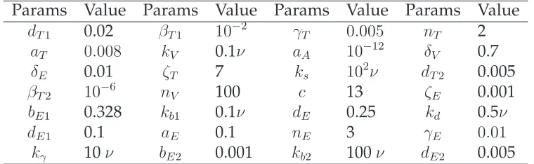
[0,100] days with parameter values given in Table 5 (adapted from Table 2 in [4]) and initial conditions
Xν(0) =ν(5,1,1400,1,10,5,1)T. (3.3)
Thus all the simulations start with the same initial concentrations(5,1,1400,1,10,5,1)T
.
Params Value Params Value Params Value Params Value
dT1 0.02 βT1 10−2 γT 0.005 nT 2
aT 0.008 kV 0.1ν aA 10−12 δV 0.7
δE 0.01 ζT 7 ks 102ν dT2 0.005
βT2 10−6 nV 100 c 13 ζE 0.001
bE1 0.328 kb1 0.1ν dE 0.25 kd 0.5ν
dE1 0.1 aE 0.1 nE 3 γE 0.01
kγ 10ν bE2 0.001 kb2 100ν dE2 0.005
Table 5: The values of parameters used in the simulation.
For the implicit tau-leaping method, the value ofǫis set as 0.12. This is chosen (based on multiple simulation results) so that the computational time is comparatively short without compromising the accuracy of the solution. In addition, the value of gi in the
tau-leaping methods is found to be
gi =
(
4, i= 2,3,4,5,6,
3, i= 1,7.
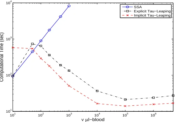
Figure 4 depicts the computational time of each algorithm for an average of five typ-ical simulation runs withν varying from 10,50,102
,2×102
,5×102
,103
for the SSA and
10,50,102
,2×102
,5×102
,103
,104
,105
,106
,5×106
for the explicit and implicit tau-leaping. From this figure, we see that the computational times for the SSA increase as the values
ν increase. This is again expected as the mean time stepsize for the SSA is the inverse of the sum of all transition rates, which increases asνincreases (roughly proportional to
ν, as can be seen from the transition rates illustrated in Table 4). In addition, even with
ν = 103
, it took the SSA more than8000 seconds for one sample path (for this reason we did not run any simulations for the SSA withνgreater than103
). Hence, it is impractical to implement the SSA if one desires to run this HIV model for a typical human (generally having5×106
µl-blood). This is not surprising due to the large value of uninfected resting CD4+ T cells (as can be seen from the initial condition (3.3)).
From Figure 4 we also see that the computational time for the explicit tau-leaping method increases as the value ν increases from 10 to 50, and decreases as ν increases to 100. Its computational time decreases dramatically as the value ofν increases from 100 to 104
, and then stabilizes there for ν ≥ 104
. This is related to the formula for τ1. As we can see from (2.3) and transition rates in Table 4, if ǫxi/gi > 1 then the first term
101 102 103 104 105 106 101
102 103 104
νµl−blood
Computational Time (sec)
SSA
Explicit Tau−Leaping Implicit Tau−Leaping
Figure 4: Comparison of computational time of different algorithm (SSA, Explicit Tau-Leaping and Implicit Tau-Tau-Leaping) for an average of five typical simulation runs.
the simulation results that the first term inside the minimum sign of (2.3) is much larger than the corresponding second term until ν = 104
, and becomes smaller than the second term when ν ≥ 104
. Hence, τ1 increases as ν increases when ν ≤ 104 and has roughly similar values for all the cases when ν ≥ 104
. This agrees with the observation that the computational time decreases dramatically as the value ofνincreases from 100 to104
, and then stabilizes forν ≥ 104
. The increase of computational time asν increases from 10 to 50 is becauseτ1 is so small that a large number of the SSA steps are implemented instead of tau-leaping.
We also observe from Figure 4 that the computational time for the implicit tau-leaping method decreases asν increases whenν ≤104
and then stabilizes forν ≥104
; this can be attributed to the same reason as in the explicit tau-leaping method. In addition, we see that the computational times for implicit tau-leaping are significantly higher than those of the SSA and explicit tau-leaping at ν = 10. This is because in this case the implicit tau-leaping is implemented for many times (solving the system of nonlinear equations in each implicit tau-leaping step is costly) and the time stepsizes are not significantly larger than those of the other two methods.
4
Concluding Remarks
In this paper we summarized comparison studies on the computational efficiency of the SSA, explicit and implicit tau-leaping methods for two distinct stochastic models with different levels of complexity. Simulation results reveal that for both models the compu-tational times of the SSA increase as the sample size (number of bedsN in the VRE model and volume of bloodνin the HIV model) increases. This is because the mean time step-size for the SSA is the inverse of the sum of the transition rates, which increases as the sample size increases. In addition, the results suggest these three algorithms have compa-rable computational times for the VRE model because of the low number of species and small number of transitions, and thus the SSA is the best choice for this problem because of its simplicity and accuracy. However, for the HIV model both tau-leaping methods have significantly lower computational cost than the SSA except when the sample sizeν
is very small (e.g., less than 100µl-blood). In addition, the implicit tau-leaping method has lower computational cost than the explicit tau-leaping method when the sample size is sufficiently large (primarily due to the stiffness of the underlying system).
Note that the stochastic HIV model in this paper describes the early infection where the number of uninfected resting T cells is very large (on order of 1000 cells perµl-blood). This explains why it required the SSA more than 8000 seconds to run one sample path with ν = 1000 µl-blood. If we assume that an average person has 5×10⁶
µl-blood, it is impractical for the SSA to run even one sample path at this scale. The numerical re-sults demonstrate that the dynamics of uninfected resting CD4+ T cells could be well approximated by ordinary differential equations even with ν = 10 µl-blood (see [3] for details). In addition, Table 5 reveals that there is a large variation between the values of the parameters. Thus, the HIV model in this paper is multi-scaled in both states and time. There are some hybrid simulation methods (also referred to as multi-scale approaches; in-terested readers can see [14] for an overview of these methods) specifically designed for multi-scale systems. The basic idea of these hybrid method is to partition the system into two subsystems, one containing fast transitions and the other containing slow transitions. Then the two subsystems are simulated iteratively by using numerical integration of ordi-nary differential equations (or stochastic differential equations) and stochastic algorithms (such as the SSA), respectively. Although these algorithms are very attractive, they are most challenging to implement and require major levels of user intervention. This is the primary reason we did not pursue these methods in our current efforts.
Acknowledgements
Num-ber NIAID R01AI071915-09 from the National Institute of Allergy and Infectious Diseases.
References
[1] L.J.S. Allen,An Introduction to Stochastic Processes with Applications to Biology, Chap-man & Hall/CRC, Boca Raton, FL, 2011.
[2] P. Bai, H.T. Banks, S. Dediu, A.Y. Govan, M. Last, A.L. Lloyd, H.K. Nguyen, M.S. Olufsen, G. Rempala and B.D. Slenning, Stochastic and deterministic models for agricultural production networks,Mathematical Biosciences and Engineering, 4 (2007), 373–402.
[3] H.T. Banks, S. Hu, M. Joyner, A. Broido, B. Canter, K. Gayvert and K. Link, A com-parison of computional efficiencies of stochastic algorithms in terms of two infection models, CRSC-TR11-13, Center for Research in Scientific Computation, North Car-olina State University, Raleigh;Math. Biosci. Engr., submitted.
[4] H.T. Banks, M. Davidian, S. Hu, G. Kepler and E.S. Rosenberg, Modelling HIV im-mune response and validation with clinical data, Journal of Biological Dynamics, 2 (2008), 357–385.
[5] Y. Cao, D.T. Gillespie and L.R. Petzold, Avoiding negative populations in explicit Poisson tau-leaping,The Journal of Chemical Physics, 123 (2005), 054104.
[6] Y. Cao, D.T. Gillespie and L.R. Petzold, Efficient step size selection for the tau-leaping simulation method,The Journal of Chemical Physics, (124) 2006, 044109.
[7] Y. Cao, D.T. Gillespie and L.R. Petzold, Adaptive explicit-implicit tau-leaping method with automatic tau selection, The Journal of Chemical Physics, 126 (2007), 224101.
[8] D.T. Gillespie, A General Method for Numerically Simulating the stochastic time evolution of coupled chemical reactions, The Journal of Computational Physics, 22 (1976), 403–434.
[9] D.T. Gillespie, Approximate accelerated stochastic simulation of chemically reacting systems,The Journal of Chemical Physics, 115 (2001), 1716–1733.
[10] D.T. Gillespie and L.R. Petzold, Improved leap-size selection for accelerated stochas-tic simulaton,The Journal of Chemical Physics, 119 (2003), 8229–8234.
[11] D.T. Gillespie and L.R. Petzold, Stochastic simulation of chemical kinetics, Annual Review of Physical Chemistry, 58 (2007), 25–55.
[13] A.R. Ortiz, H.T. Banks, C. Castillo-Chavez, G. Chowell and X. Wang, A deterministic methodology for estimation of parameters in dynamic Markov chain models,Journal of Biological Systems, 19 (2011), 71–100.
[14] J. Pahle, Biochemical simulations: stochastic, approximate stochastic and hybrid ap-proaches,Brief Bioinform, 10 (2009), 53–64.
[15] M. Rathinam, L.R. Petzold, Y. Cao and D.T. Gillespie, Stiffness in stochastic chem-ically reacting systems: the implicit tau-leaping method, The Journal of Chemical Physics, 119 (2003), 12784–12794.
[16] E. Renshaw,Modelling Biological Populations in Space and Time, Cambridge Univ. Press, 1991.