DEPARTMENT OF STATISTICS
North Carolina State University
2501 Founders Drive, Campus Box 8203
Raleigh, NC 27695-8203
Institute of Statistics Mimeo Series No. 2605
Simultaneous factor selection and collapsing levels in
ANOVA
Howard D. Bondell and Brian J. Reich
Department of Statistics, North Carolina State University
Raleigh, NC 27695-8203, U.S.A.
Simultaneous factor selection and collapsing levels in
ANOVA
Howard D. Bondell and Brian J. Reich
Department of Statistics, North Carolina State University,
Raleigh, NC 27695-8203, U.S.A.
October 1, 2007
Summary. When performing an Analysis of Variance, the investigator often has two main
goals: to determine which of the factors have a significant effect on the response, and to
detect differences among the levels of the significant factors. Level comparisons are done
via a post-hoc analysis based on pairwise differences. One common complaint about this
approach is that the levels are not necessarily collapsed into non-overlapping groups. This
paper proposes a novel constrained regression approach to simultaneously accomplish both
goals via shrinkage within a single automated procedure. The form of this shrinkage has
the ability to collapse levels within a factor by setting their effects to be equal, while also
achieving factor selection by zeroing out entire factors. Using this approach also leads to the
identification of a structure within each factor, as levels can be automatically collapsed to
form groups. In contrast to the traditional pairwise comparison methods, these groups are
necessarily non-overlapping so that the results are interpretable in terms of distinct subsets
of levels. The proposed procedure is shown to perform well in simulations and in a real data
example.
Key words: ANOVA; Grouping; Multiple comparisons; Shrinkage; Variable selection.
1. Introduction
Analysis of Variance (ANOVA) is a commonly used statistical technique to determine a
relationship between a continuous response and categorical predictors. ANOVA is
particu-larly applicable to designed experiments where the focus is on discovering the relevant factors
that affect the response. An initial goal in ANOVA is to judge the overall importance of
these categorical factors. If a factor is deemed important, a secondary analysis is performed
to determine which levels of an important factor really differ from one another and which do
not. This second question is typically answered via a post-hoc analysis involving pairwise
comparisons within factors that are found to be important. Some common approaches to
judge significance when the pairwise comparisons are considered include Tukey’s Honestly
Significantly Different (HSD) test, Fisher’s Least Significant Difference (LSD) procedure,
Bonferroni or Scheffe multiple comparison adjustments, and more recently, procedures based
on the False Discovery Rate (Benjamini and Hochberg, 1995; Storey, 2002). One common
complaint of applied scientists in this type of analysis is that it is often not possible to
collapse the levels into non-overlapping groups based on the pairwise difference results.
Accomplishing the goal of judging importance of the factor levels is a variable selection
problem that has received a great deal of attention in the literature. In particular,
penal-ized, or constrained, regression has emerged as a highly-successful technique for variable
selection. For example, the LASSO (Tibshirani, 1996) imposes a bound on the L1 norm
of the coefficients. This results in both shrinkage and variable selection due to the nature
of the constraint region which often results in several coefficients becoming identically zero.
Alternative choices of constraints, or penalties, have also been proposed for shrinkage and
selection in regression (Frank and Friedman, 1993; Fan and Li, 2001; Tibshirani et al., 2005;
Zou and Hastie, 2005; Bondell and Reich, 2006; Zou, 2006).
typically coded in terms of dummy variables, as opposed to a single coefficient as in the
case of regression using continuous predictors. Naive use of a penalization technique does
not achieve variable selection properly in this situation, as it can set some of the dummy
variables corresponding to a factor to zero, while others are not. Yuan and Lin (2006) propose
the Group LASSO in order to perform variable selection for entire factors by appropriately
treating these dummy variables as a group and constraining the sum of group norms as
opposed to a single overall norm. This approach accomplishes the first goal in ANOVA
of selecting the important factors. However, the post-hoc analysis of pairwise comparisons
must still be performed, as it is not built in to this procedure. For each significant factor,
each of the dummy variables will be given a distinct coefficient in the estimated model.
A novel constrained regression approach called CAS-ANOVA (for Collapsing And
Shrink-age in ANOVA) is proposed in this paper to simultaneously perform the two main goals of
ANOVA within the estimation procedure. The form of the constraint encourages similar
effect sizes within a factor to be estimated with exact equality, thus collapsing the
corre-sponding levels. In addition, via the typical ANOVA design parametrization combined with
this constraint, entire factors can be collapsed to a zero effect, hence providing the desired
factor selection. In this manner, the proposed procedure allows the investigator to
con-duct a complete analysis on both the factors and the individual levels in a single step, thus
eliminating the need for a secondary analysis.
In addition to performing the collapsing of levels within the estimation procedure itself,
another important distinction between this CAS-ANOVA approach and the typical
post-hoc pairwise comparison approach is that the typical approaches in many instances will
not actually yield a feasible collapsing of levels, whereas in the proposed procedure, this is
automatic. As a simple example, in a typical ANOVA analysis for a factor with 3 levels,
significantly different from level 3. This result would not correspond to any possible way of
grouping the three levels, whereas in the proposed procedure, this infeasible grouping cannot
occur, as the structure is incorporated into the estimation procedure.
This procedure requires a single tuning parameter to control the degree of shrinkage.
Various methods to choose this parameter are discussed including a new technique to tune
the procedure based on a notion of False Selection rate. The intuitive idea is to add false
differences to the data. This is accomplished by artificially splitting cells of the design and
monitoring how well the procedure fuses them back together.
The remainder of the paper proceeds as follows. The CAS-ANOVA procedure is
intro-duced in §2, while computation and a data adaptive version of the procedure are discussed
in§3. Techniques for tuning the procedure including a novel procedure based on estimating
the False Selection Rate appear in §4. Finally, §5 gives a simulation study and a real data
example.
2. Collapsing And Shrinkage in ANOVA
2.1 The procedure
To establish notation, consider the additive ANOVA model with J factors and a total sample size n. Factor j has pj levels, and denote p=
PJ
j=1pj. Letn
(k)
j be the total number
of observations with factor j at level k, for k = 1, ..., pj and j = 1, ..., J. Under a balanced
design this simplifies to n(jk) =nj =n/pj for all k.
Assume that the responses have been centered to have mean zero, so that the intercept
can be omitted in the case of a balanced design. Let the n ×p design matrix X be the typical over-parameterized ANOVA design matrix composed of zeros and ones denoting the
combination of levels for each of the n observations. This parametrization is useful for this approach as equality of coefficients correspond exactly to collapsing levels.
esti-mates the p coefficients, which can be interpreted as the effect sizes for each level, by the solution to
ˆ
βββ = arg minβββ||y−Xβββ||2
subject to
Ppj
k=1βjk= 0 for all j = 1, ..., J,
(1)
where the constraint forces the effects for the levels within each factor to sum to zero for
identifiability.
An additional constraint can then be added to this optimization problem to shrink the
coefficients in order to perform variable selection, such as the LASSO, or Group LASSO. To
perform the collapsing of levels, a desirable constraint would not only have the ability to set
entire groups to zero, it would additionally be able to collapse the factor levels by setting
subsets of coefficients within a group to be equal. For the linear regression setting, the
OSCAR (Bondell and Reich, 2006) uses a mixture of L1 and pairwise L∞ penalty terms to
simultaneously perform variable selection and find clusters among the important predictors.
The nature of this penalty naturally handles both positive and negative correlations among
continuous predictors, which does not come into play in the ANOVA design.
With the ANOVA goals in mind, the proposed CAS-ANOVA procedure places a
con-straint directly on the pairwise differences as
˜
βββ = arg minβββ||y−Xβββ||2
subject to
Ppj
k=1βjk= 0 for all j = 1, ..., J and
PJ
j=1
P
1≤k<m≤pjw
(km)
j |βjk−βjm| ≤t,
(2)
wheret >0 is a tuning constant andw(jkm) is a weight for the pair of levelsk andmof factor
j. These weights are needed to account for the fact that the number of levels for each factor are not necessarily the same and that the design may also be unbalanced. In the balanced
design case, the weights for all pairs of levels within a given factor would be equal, so in that
case w(jkm) =wj. An appropriate choice of weights is discussed in the next section.
each factor used in the standard ANOVA. The second constraint is a generalized version of
the Fused LASSO-type constraint (Tibshirani et al., 2005) taken on the pairwise differences
within each factor. The Fused LASSO itself constrains consecutive differences in the
regres-sion setting to yield a smoother coefficient profile for ordered coefficients. Here the pairwise
constraints smooth the within factor differences towards one another. This second constraint
enables the automated collapsing of levels within the factor. In addition, combining the two
constraints implies that entire factors will be set to zero once their levels are collapsed.
As opposed to the typical pairwise comparison methods, this approach will automatically
yield non-overlapping groups so that a feasible group structure among the levels of a factor
will always emerge. This additional benefit alleviates the common problem faced by applied
scientists in the interpretation of the post-hoc analysis.
2.2 Choosing the weights
In any penalized regression, having each predictor on a comparable scale is essential so
that the predictors are penalized equally. This is typically done by standardization, so that
each column of the design matrix has its 2-norm equal unity. This could instead be done by
weighting each term of the penalty as in (2). Clearly, when the penalty is based on a norm,
rescaling a column of the design matrix is equivalent to instead weighting the corresponding
coefficient in the penalty term by the inverse of this rescaling factor. In standard situations
such as the LASSO, each column contributes equally to the penalty, so it is clear how
to standardize the columns (or, equivalently, weight the terms in the penalty). However,
standardizing the predictors in the CAS-ANOVA procedure is not as straightforward, as the
penalization involves the pairwise differences. Although the design matrix consists of only
zeros and ones, the number of terms in the penalty changes dramatically with the number
of levels per factor, while the amount of information in the data to estimate each coefficient
It is now shown that an appropriate set of weights to use in the CAS-ANOVA procedure
(2) are
wj(km) = (pj+ 1)−1
q
n(jk)+n
(m)
j , (3)
which for the special case of the balanced design would be wj = (pj + 1)−1
p
2nj. The idea
behind these weights is based on the notion of ‘standardized predictors’ as follows.
Let θθθ denote the vector of the pairwise differences taken within each factor. Hence θθθ
is a vector of length d = PJ
j=1dj =
PJ
j=1pj(pj −1)/2. Let the over-parameterized model
withq =p+dparameters arising from thepcoefficients plus the d pairwise differences have parameter vector denoted by
γγγ =Mβββ = βββT1, θθθ
T
1, . . . , βββ
T J, θθθ
T J
T
,
whereβββj andθθθj are the coefficients and pairwise differences corresponding to factor j. The
matrix M is block diagonal withjth block given by M
j = [Ipj×pj D
T
j]T, withDj the dj ×pj
matrix of ±1 that creates the vectorθθθj fromβββj for a given factor j by picking off each of
the pairwise differences from that factor.
The corresponding design matrix Z for this overparameterized design is then an n×q
matrix such that Zγγγ =Xβββ for allβββ. Hence it is desired to solve ZM =X. ClearlyZ is not uniquely defined. An uninteresting choice would be Z = [X 0n×d]. Also, Z = XM∗, with
M∗ as any left inverse ofM, would suffice. We choose
Z =XM−,
where M− denotes the Moore-Penrose generalized inverse of M. This resulting matrix Z is
an appropriate design matrix for the overparamterized space. One could directly work with
after standardization would no longer have the same interpretation as differences between
effects, so that collapsing levels is no longer accomplished. Hence the corresponding approach
to weighting the terms in the penalty is advocated. The appropriate weights are then just
the Euclidean norm of the columns of Z that correspond to each of the differences. It can be shown that the proposed weights are exactly these norms.
Proposition. The Moore-Penrose generalized inverse of the matrix M is block diagonal
with the jth diagonal block corresponding to the jth factor and of the form (M−)
j = (pj+
1)−1[(I
pj×pj+1pj1
T pj) D
T
j ]. Furthermore, under the ANOVA design, the column ofZ =XM−
that corresponds to the difference in effect for levelsk and mof factorj has Euclidean norm (pj+ 1)−1
q
n(jk)+n(jm).
The above proposition, whose proof is given in the appendix, allows the determination
of the weights via the standardization in this new design space. Under the balanced design,
the weights only depend on the factor regardless of the levels considered, whereas that is not
the case in the unbalanced design.
Note that standardizing the columns of Z and imposing an L1 penalty on θθθ as in the
typical LASSO approach (Tibshirani, 1996), is strictly equivalent to choosing the weights to
be the Euclidean norm of the corresponding column only when the columns have mean zero.
Now for the matrixZ, the columns corresponding to a difference consist of elements given by {0,±(pj + 1)−1}, and the mean of each of these columns is given by{n(pj+1)}−1{n(
k)
j −n
(m)
j },
so that under the balanced design the columns have mean zero. Meanwhile, in an unbalanced
design, the weighting is at least approximately equivalent to standardization, as the mean
3. Computation
The CAS-ANOVA optimization problem can be expressed as a quadratic programming
problem as follows. For each k = 1, ..., d, set θk =θk+−θ
−
k with both θ
+
k and θ
−
k being
non-negative, and only one is nonzero. Then |θk|=θk++θ
−
k. Now let the full p+ 2ddimensional
parameter vector be denoted byη. For each factorj, letX∗
j = [Xj 0n×2dj], whereXj denotes
the columns of the design matrix corresponding to factor j and dj = pj(pj − 1)/2 is the
number of differences for factorj. Then let X∗ = [X∗
1...XJ∗] be then×(p+ 2d) dimensional
design matrix formed by combining all of the X∗
j. Then X∗η = Xβ. The optimization
problem can be written as
˜
η= arg minη||y−X∗η||2
subject to
Lη= 0, Pd
k=1w(k)(θk++θ
−
k)≤t and θ+k, θ
−
k ≥0 for all k = 1, ..., d,
(4)
wherew(k) denotes the weight for pairwise difference k and the matrix Lis a block diagonal
matrix with jth block L
j givenby
Lj =
Dj Idj −Idj
1T pj 0
T dj 0
T dj
for each j = 1, ..., J.
The optimization problem given by (4) is just a standard quadratic programming problem
as all constraints are linear. This quadratic programming problem has p+ 2d parameters and p+ 3d linear constraints. Note that both the number of parameters and constraints grow withp, but the growth is not quadratic in p, it is only quadratic in the number of levels within a factor, which is typically not too large. Hence this direct computational algorithm
is feasible for the majority of practical problems.
4. An adaptive CAS-ANOVA
It has been shown both theoretically and in practice that a weighted version of the LASSO
of selecting the correct model and not overshrinking large coefficients (Zou, 2006). The
intuition is to weight each coefficient in the penalty so that estimates of larger coefficients
are penalized less and in the limiting case, coefficients that are truly zero will be infinitely
penalized unless the estimate is identically zero. Specifically the optimization problem for
the adaptive LASSO is given by
˜
βββ = arg minβββ||y−Xβββ||2
subject to
Pp
k=1|βˆk|−1|βk| ≤t,
(5)
where ˆβk denotes the ordinary least squares estimate for βk. The idea is that the weights
for the non-zero components will converge to constants, whereas the weights for the zero
components diverge to infinity. Zou (2006) has shown that if the bound is chosen
appro-priately, the resulting estimator has the oracle property in that it obtains consistency in
variable selection along with asymptotic efficiency for the non-zero components.
This approach can also be used here directly by modifying the CAS-ANOVA optimization
problem given by (2) as
˜
βββA= arg minβββ||y−Xβββ||2
subject to
Ppj
k=1βjk= 0 for all j = 1, ..., J and PJj=1P1≤k<m≤pjw
(km)∗
j |βjk−βjm| ≤t,
(6)
where
wj(km)∗ =wj(km)|βˆjk−βˆjm|−1,
with w(jkm) as in (3), and the vector ˆβββ denotes the estimate obtained from the typical least squares ANOVA with the sum to zero constraint as given by (1). This is exactly the adaptive
LASSO on the space of pairwise differences.
Note that computationally, a single ANOVA fit is done initially and the weight for each
difference is adjusted based on this fit as above. Then the computation in the adaptive
5. Tuning the procedure
5.1 Cross-validation and degrees of freedom
In general penalized, or constrained, regression techniques, one must choose the value of
the tuning parameter, the boundtin this case. The choice oft yields a trade-off of fit to the data with model complexity, or sparsity. This choice can be accomplished via minimizing
any of the standard techniques to estimate out-of-sample prediction error, such as AIC, BIC,
Generalized Cross-Validation (GCV), or directly via k-fold Cross-Validation. To use any of
the criteria such as AIC, BIC, or GCV, an estimate of the number of degrees of freedom is
needed. For the LASSO, it is known that the number of non-zero coefficients is an unbiased
estimate of the degrees of freedom (Zou et al., 2004). For the Fused LASSO (Tibshirani et
al., 2005), the number of non-zero blocks of coefficients is used as an estimate of degrees of
freedom. In this ANOVA design case, the natural estimate of degrees of freedom for each
factor is the number of unique coefficients minus one for the constraint, this represents the
number of resulting levels minus one. Specifically, one has
ˆ df =
J
X
j=1
p∗
j −1
, (7)
where p∗
j denotes the number of estimated unique coefficients for factorj.
5.2 False selection rate
Using prediction error to judge the fit in order to choose the tuning parameter is not
necessarily the most appropriate measure when the main goal in the ANOVA analysis is to
determine the important factors and levels. In keeping with this goal, an alternative tuning
procedure is now introduced for the CAS-ANOVA procedure based on the idea of False
Selection Rate (FSR) as proposed in the context of variable selection by Wu et al. (2006).
FSR in variable selection is the analogue of False Discovery Rate (FDR) in that it measures
the proportion of unimportant variables selected, U(X, Y), out of the total number selected,
made explicit, and the 1 in the denominator reflects the inclusion of an intercept and also
avoids division by zero in the case that no variables are selected.
However, which of the variables are truly important or unimportant is, of course,
un-known, so that the number of unimportant variables selected by a procedure, U(X, Y), is not known and must somehow be estimated. The approach of Wu et al. (2006) is to
gen-erate new data sets by appending known irrelevant variables to the original data and, for a
given tuning parameter, monitor the proportion of these variables that are selected out of
the total number of selected variables, on average. Under some simplifying assumptions, a
multiplicative factor is derived to obtain a direct estimate of the FSR for the original data
set corresponding to that tuning parameter. One then chooses the tuning parameter that
selects the largest model whose estimated FSR, ˆγ, remains below a desired level, typically
γ0 = 0.05. This idea is intuitively appealing for this situation as it is more in line with the
goals of ANOVA, as opposed to a criterion based on prediction error.
Specifically, the method of Wu et al. (2006) proposes to estimate the FSR for a given
tuning parametert as
ˆ
γ = kˆUU¯
∗
P/kP
1 +S(X, Y, t), (8) where ˆkU is the estimated number of truly unimportant variables in the original data set, ¯UP∗
is the average number of known irrelevant variables that were selected from the appended
data sets, kP denotes the number of irrelevant variables that were appended to create each
new data set, and the dependence on the tuning parameter t is made explicit.
However, simply adding extra variables to the ANOVA design matrix is not directly
applicable for tuning this procedure, as just adding additional factors is not sufficient to
also judge the collapsing of levels. Instead, a novel method is proposed to implicitly add
new differences that are known to be zero and monitor the FSR on the full set of pairwise
comparisons with the currently used methods. However, with the proposed CAS-ANOVA
technique, this is accomplished simultaneously within the estimation procedure where the
pairwise differences from all factors, including those that are set to zero, is taken into account
by the FSR.
To fix ideas, consider the replicated balanced ANOVA design so that there arec=QJ
j=1pj
total combinations (cells), each having r > 1 observations. To effectively add these known irrelevant differences, the proposed method splits each cell of the ANOVA table as follows.
Letννν be a c×1 vector of parameters, then a derived new model is
y=Xβββ+Aννν+,
with the matrix A containing elements given by {0,±1/2} that randomly splits the obser-vations for each cell into two groups of size r/2.
Remark: This idea naturally generalizes to unequally splitting of cells if r is odd or if the design is unbalanced, including splitting of only some cells if there are replications for
some combinations but not for others. Additionally, splitting could be into multiple groups
if there were a large number of replications thus obtaining more irrelevant differences. This
approach to tuning the procedure does require that there are replications of at least some
combinations so that it is possible to divide at least some of the cells.
As parameterized, the vector ννν represents the differences in predicted response between each half of the split cells, which plays exactly the role that the pairwise differences play.
Hence for estimation in this derived model, each of the |νj| is penalized along with θθθ, the
vector of pairwise differences, in (2) and thus the matrix Aplays the role of adding the irrel-evant difference variables to the full vector of pairwise differences. Using the standardization
idea, assuming a balanced design and equal splitting of each cell into two groups, the weight
of A.
Now for a given tuning parameter t, one estimates the full vector (βββ, θθθ, ννν) based on the matrix A corresponding to a possible splitting of the cells. The number of total nonzero estimates of elements ofννν then plays the role of U∗
P, the number of chosen irrelevant
differ-ences. Note that ifr= 2 there is only one split possible so that the term ¯U∗
P used to estimate
the FSR is based solely on the number of nonzero estimates of the components ofννν for this split. If r >2 then the cells can be split in multiple ways so that ¯U∗
P is based on averaging
the number of nonzero estimates over the splits, either via all possible splits, or by random
splits.
Remark: This approach to tuning is not advocated for the adaptive CAS-ANOVA as,
in that case, one must also adaptively weight each |νj|. These weights would be different
depending on the split, thus changing the meaning of the tuning parameter t for each split.
This method proposed to estimate the FSR by Wu et al. (2006) is based on the
assump-tion that on average, the real unimportant variables and the added unimportant variables
have the same probability of being selected. Wu et al. (2006) recognize that this assumption
is almost surely to be violated and only claim the method to be an approximation. In this
ANOVA setting, since the ‘variables’ under consideration are actually the pairwise
differ-ences and hence tied together in a complex manner, this assumption is even less likely to
hold. However, the simulation results in the next section show that, although it is only an
approximation, tuning the CAS-ANOVA procedure in this manner works well in practice for
control of the FSR.
6. Examples
6.1 Simulation study
A simulation study was carried out to examine the performance of the CAS-ANOVA
The first example is a three-factor experiment having 8, 4, and 3 levels respectively. The
response is generated to have overall mean zero and true effect vector for the first factor given
by β = (2,2,−1,−1,−1,−1,0,0)T and the remaining two factors have zero effect. The first
factor truly has 3 distinct subgroups, hence an ‘oracle’ procedure would eliminate the two
extraneous factors and collapse the 8 levels into 3 groups. The simulation was done for a
balanced design with a single observation per combination, and then repeated for the two
additional cases of 2 and 4 replications per combination.
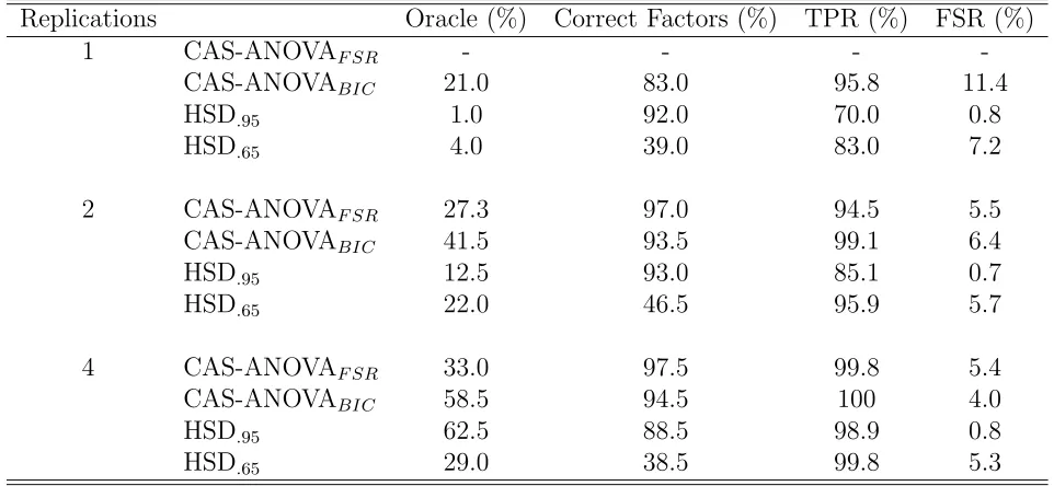
Table 1 compares the standard version tuned by AIC, BIC, and GCV, with the adaptive
version tuned in the analagous manner for this example. ‘Oracle’ represents the percent
of time the procedure chose the fully correct model in terms of which factors should be
eliminated and which levels collapsed. ‘Correct Factors’ represents the percent of time that
the complete nonsignificant factors are eliminated and the true factors are kept. True Positive
Rate (TPR) represents the average percent of true differences found (out of the 20 total true
differences), whereas FSR represents the average percent of declared differences that are
mistaken (the observed False Selection Rate).
***** TABLE 1 GOES HERE ******
Clearly, the adaptive weights yield a large improvement in terms of the model selection as
expected. In addition, the adaptive version using BIC is much preferred as the other criteria
regularly choose too large of a model. This was seen in each of the examples that were tried,
so that for the remainder of the simulations and real example, the adaptive version tuned
via BIC is the method used, and is the method recommended in practice.
Table 2 shows the results for the proposed procedure (CAS-ANOVA) tuned via
estimated FSR of 0.05 in the standard CAS-ANOVA procedure. Additionally is shown the results for the proposed adaptive version of the procedure tuned via BIC. Note that the
CAS-ANOVA procedure tuned via the FSR is not applicable for the unreplicated design so
the corresponding entries in the table are omitted. It is also again noted that the adaptive
version tuned via FSR is not appropriate to choose the tuning parameter, as this parameter
does not have the same meaning in each newly created data set.
Tukey’s HSD procedure based on the 95% confidence level is shown for comparison. As
seen in the table, the HSD procedure is overly conservative in terms of its FSR and is thus
selecting a smaller model in general. This is seen from the much lower TPR and Oracle. The
HSD procedure using the 65% confidence level was empirically found to yield an approximate
FSR of 0.05, and thus is given as an additional comparison. This procedure is too aggressive in that too many terms are included in the model. This can be seen by the poor performance
in not dropping the irrelevant factors often enough. Additionally, the fact that impossible
grouping structures can be found by the HSD procedures help to contribute to the lower
percentages of selecting the true model (‘Oracle’). Overall, the CAS-ANOVA procedures
tuned by both methods do a good job in picking out the appropriate model structure. For
larger samples, the adaptive version tuned via BIC exhibits better performance than that of
tuning by FSR, but does not allow for control of the error rate. The tuning by FSR allows
the user to approximately control the error rate, but cannot be used in all situations.
***** TABLE 2 GOES HERE ******
A second simulation setup with 4 factors having smaller effect sizes was also examined.
Again the response has overall mean zero with the first two factors having effects given by
β1 = (.75, .75,−.5,−.5,−.5,0)T andβ2 = (.25, .25,−.5)T, respectively. The other two factors
Table 3 shows the results of this simulation for the CAS-ANOVA procedure tuned by
the two previous methods, as well as the two versions of Tukey’s HSD. Again one can see
that the newly proposed method does well at accurately detecting the underlying model
structure.
***** TABLE 3 GOES HERE ******
6.2 Real data example
The data for this example comes from a three-way analysis of variance for yields of
barley. The response is the barley yield for each of five varieties at six experimental farms
in Minnesota for each of the years 1931 and 1932 giving a total of 60 observations. Note
that there is a single observation for each variety/location/year combination representing
the total barley yield for that combination. This data was first introduced by Immer et al.
(1934), and variations of this dataset have been used by Fisher (1971), Cleveland (1993) and
Venables and Ripley (2002).
A practitioner would proceed by conducting an overall analysis of variance to decide on
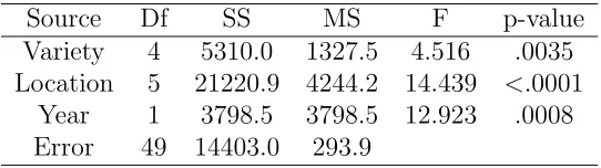
the significant factors. The standard ANOVA table for testing the overall factors is given in
Table 4. Clearly all three factors are significant, so a typical analysis would next proceed by
considering the pairwise differences to determine which factor levels differ from one another.
To accomplish this goal, a post-hoc analysis using Tukey’s HSD procedure at both the .95
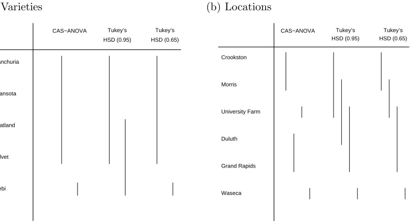
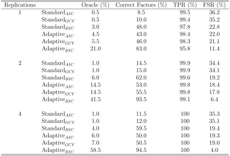
and the .65 levels was performed and is plotted in Figure 1. Tukey’s procedure (at both
confidence levels) produces overlapping groups of levels for the location factor (Figure 1b).
For example, Tukey’s procedure finds that the Morris and Duluth locations are significantly
different, but neither location significantly differs from the University Farm.
Instead of performing a first analysis to determine significance and then the post-hoc
Table 4: ANOVA table for the barley data.
Source Df SS MS F p-value Variety 4 5310.0 1327.5 4.516 .0035 Location 5 21220.9 4244.2 14.439 <.0001
Year 1 3798.5 3798.5 12.923 .0008 Error 49 14403.0 293.9
single combined analysis. Since there is no replication, the tuning via FSR is not applicable,
so the adaptive version of the procedure tuned via BIC was used. As with the standard
ANOVA, the CAS-ANOVA procedure includes all three factors. The grouping structure is
shown in Figure 1. By construction, the groups are non-overlapping. The overlapping-group
problem of Tukey’s procedure is resolved by creating a separate group for the University
Farm.
***** FIGURE 1 GOES HERE ******
Based on the simulations and the real data example, the new proposal of this paper
appears to be a competitive alternative to the standard post-hoc analysis in ANOVA. An
additional benefit is that it allows the investigator to directly determine a grouping structure
among the levels of a factor that may not be clearly demonstrated by using a standard
pairwise comparison procedure.
7. Discussion
This paper has proposed a new procedure to simultaneously include pairwise comparisons
into the estimation procedure when performing an analysis of variance. By combining the
overall testing with the collapsing of levels, it creates distinct groups of levels within a
structure. The procedure avoids the use of multiple testing corrections by performing the
comparisons directly. In the case of a design with replication, a tuning method based on
the idea of controlling False Selection Rate has been introduced. In cases with or without
replication, the reweighted version of this procedure with tuning parameter chosen via BIC
has shown strong performance.
In a similar manner, if desired, the collapsing of levels can be accomplished on interaction
terms as well. Currently an approach to collapse levels in a hierarchical framework is under
investigation. In this case it may be desired to collapse two levels of a main effect only if
it is also reasonable to completely collapse all interactions of those two levels with each of
the other terms. This enforcing of the hierarchical structure would require a more complex
penalty form.
An additional important idea from this approach is that, in general, it may be possible
to combine individual components of an analysis into a single step by an appropriately
constructed constraint, or penalty function. In this manner, constrained regression can be
tailored to accomplish multiple statistical goals simultaneously.
The ANOVA model has also been revisited recently from the Bayesian perspective. For
example, Nobile and Green (2000) model the factor levels as draws from a mixture
distri-bution, thus ensuring non-overlapping levels at each MCMC iteration. The CAS-ANOVA
procedure also has a Bayesian interpretation. The CAS-ANOVA solution is the posterior
mode assuming each factor’s levels have a Markov random field prior (popularized for spatial
modelling by Besag et al., 1991) with L1-norm, i.e.,
p(βββj)∝exp
−λ X
1≤k<m≤pj wkm
j |βjk−βjm|
,
Appendix
Proof of Proposition 1.
The matrix M is block diagonal withjth block given by M
j = [Ipj×pj D
T
j ]T, with Dj the
d×pj matrix of ±1 that picks off each of the pairwise differences from factor j. Hence it
suffices to consider each block individually. Consider the matrix M−
j = (pj+ 1)−1[(Ipj×pj+
1pj1
T pj) D
T
j ]. ThenM
−
j Mj = (pj+1)−1[(Ipj×pj+1pj1
T pj)+D
T
j Dj]. Now via direct calculation,
one obtains DT
j Dj =pjIpj×pj −1pj1
T
pj, so thatM
−
j Mj =Ipj×pj.
Now to show that M−
j is the Moore-Penrose inverse of Mj, it suffices to show
1. M−
j MjMj−=M
−
j .
2. MjMj−Mj =Mj.
3. M−
j Mj is symmetric.
4. MjMj− is symmetric.
Clearly (1), (2), and (3) follow directly from the fact that M−
j Mj =Ipj×pj. For (4),
MjMj− = (pj + 1)−1
(Ipj×pj+1pj1
T
pj) D
T j
Dj(Ipj×pj +1pj1
T
pj) DjD
T j
.
Now from the form of Dj, it follows that Dj1pj1
T
pj = 0d×pj. Thus the matrix is symmetric.
Hence M− is the Moore-Penrose inverse of M. The Euclidean norm of the columns of
Z = XM− corresponding to the differences follows directly, as these columns of Z contain
References
Benjamini, Y. and Hochberg, Y. (1995), Controlling the false discovery rate: a practical and
powerful approach to multiple testing, Journal of the Royal Statistical Society B, 57,
289-300.
Besag, J., York, J. C., and Molli´e, A (1991), Bayesian image restoration, with two
ap-plications in spatial statistics (with discussion), Annals of the Institute of Statistical
Mathematics, 43, 1-59.
Bondell, H. D. and Reich, B. J. (2006), Simultaneous regression shrinkage, variable selection
and clustering of predictors with OSCAR, Institute of Statistics Mimeo Series # 2583,
North Carolina State University.
Cleveland, W. S. (1993), Visualizing Data, New Jersey: Hobart Press.
Fan, J. and Li, R. (2001), Variable selection via nonconcave penalized likelihood and its
oracle property, Journal of the American Statistical Association, 96, 1348-1360.
Fisher, R. A. (1971),The Design of Experiments, New York: Hafner, 9th edition.
Frank, I. E. and Friedman, J. (1993), A statistical view of some chemometrics regression
tools,Technometrics, 35, 109148.
Immer, F. R., Hayes, H. D., and Powers, L. (1934), Statistical determination of barley
varietal adaptation,Journal of the American Society for Agronomy, 26, 403419
Nobile, A. and Green, P. J. (2000), Bayesian analysis of factorial experiments by mixture
modelling, Biometrika, 87, 15-35.
Storey, J. D. (2002), A direct approach to false discovery rates, Journal of the Royal
Statis-tical Society B, 64, 479-498.
Tibshirani, R. (1996), Regression shrinkage and selection via the lasso, Journal of the Royal
Statistical Society B, 58, 267-288.
smooth-ness via the fused lasso, Journal of the Royal Statistical Society B, 67, 91-108.
Venables, W. N. and Ripley, B. D. (2002), Modern Applied Statistics with S, New York:
Springer, 4th edition.
Wu, Y., Boos, D. D. and Stefanski, L. A. (2006), Controlling Variable Selection By the
Addition of Pseudo-Variables,Journal of the American Statistical Association,102,
235-243.
Yuan, M. and Lin, Y. (2006), Model selection and estimation in regression with grouped
variables,Journal of the Royal Statistical Society B, 68, 49-67.
Zou, H. (2006), The adaptive LASSO and its oracle properties, Journal of the American
Statistical Association, 101, 1418-1429.
Zou, H. and Hastie, T. (2005), Regularization and variable selection via the elastic net,
Journal of the Royal Statistical Society B, 67, 301-320.
Zou, H., Hastie, T., and Tibshirani, R. (2004), On the degrees of freedom of the lasso,
Figure 1: Group structure for the barley data using Tukey’s HSD (with 95% and 65% confidence levels) and CAS-ANOVA. Each vertical line represents a set of levels that are grouped.
Manchuria
Svansota
Peatland
Velvet
Trebi
CAS−ANOVA Tukey’s HSD (0.95)
Tukey’s HSD (0.65)
Crookston
Morris
University Farm
Duluth
Grand Rapids
Waseca
CAS−ANOVA Tukey’s HSD (0.95)
Table 1: Example 1. Comparison of the adaptive and standard CAS-ANOVA procedures for the selection criteria AIC, BIC, and GCV. Oracle represents the percent of time the procedure chose the entirely correct model. Correct Factors represents the percent of time the nonsignificant factors are completely removed. TPR represents the average percent of true differences found, whereas FSR represents the average percent of declared differences that are mistaken.
Replications Oracle (%) Correct Factors (%) TPR (%) FSR (%)
1 StandardAIC 0.5 8.5 99.5 36.2
StandardGCV 0.5 10.0 99.4 35.2
StandardBIC 3.0 48.0 97.8 22.8
AdaptiveAIC 4.5 43.0 98.4 22.0
AdaptiveGCV 5.5 46.0 98.3 21.1
AdaptiveBIC 21.0 83.0 95.8 11.4
2 StandardAIC 1.0 14.5 99.9 34.4
StandardGCV 1.0 15.0 99.9 34.1
StandardBIC 6.0 62.0 99.6 19.2
AdaptiveAIC 14.5 53.0 99.8 18.4
AdaptiveGCV 14.5 55.5 99.8 17.8
AdaptiveBIC 41.5 93.5 99.1 6.4
4 StandardAIC 1.0 11.5 100 35.3
StandardGCV 1.0 12.0 100 35.1
StandardBIC 4.0 59.5 100 19.4
AdaptiveAIC 6.0 50.0 100 19.3
AdaptiveGCV 7.0 50.5 100 19.0
Table 2: Example 1. Performance of the CAS-ANOVA procedure using the False Selection Rate criterion and the adaptive CAS-ANOVA procedure using BIC. Tukey’s Honestly Sig-nificant Difference (HSD) is shown for comparison. Oracle represents the percent of time the procedure chose the entirely correct model. Correct Factors represents the percent of time the nonsignificant factors completely removed. TPR represents the average percent of true differences found, whereas FSR represents the average percent of declared differences that are mistaken.
Replications Oracle (%) Correct Factors (%) TPR (%) FSR (%)
1 CAS-ANOVAF SR - - -
-CAS-ANOVABIC 21.0 83.0 95.8 11.4
HSD.95 1.0 92.0 70.0 0.8
HSD.65 4.0 39.0 83.0 7.2
2 CAS-ANOVAF SR 27.3 97.0 94.5 5.5
CAS-ANOVABIC 41.5 93.5 99.1 6.4
HSD.95 12.5 93.0 85.1 0.7
HSD.65 22.0 46.5 95.9 5.7
4 CAS-ANOVAF SR 33.0 97.5 99.8 5.4
CAS-ANOVABIC 58.5 94.5 100 4.0
HSD.95 62.5 88.5 98.9 0.8
Table 3: Example 2. Performance of the CAS-ANOVA procedure using the False Selection Rate criterion and the adaptive CAS-ANOVA procedure using BIC. Tukey’s Honestly Sig-nificant Difference (HSD) is shown for comparison. Oracle represents the percent of time the procedure chose the entirely correct model. Correct Factors represents the percent of time the nonsignificant factors are completely removed. TPR represents the average percent of true differences found, whereas FSR represents the average percent of declared differences that are mistaken.
Replications Oracle (%) Correct Factors (%) TPR (%) FSR (%)
1 CAS-ANOVAF SR - - -
-CAS-ANOVABIC 15.5 86.0 89.3 11.0
HSD.95 0 89.0 67.1 1.8
HSD.65 0.5 43.0 81.4 10.7
2 CAS-ANOVAF SR 25.0 94.5 89.7 5.9
CAS-ANOVABIC 35.5 87.0 95.1 7.4
HSD.95 4.5 90.0 82.1 1.4
HSD.65 11.0 38.0 91.7 10.4
4 CAS-ANOVAF SR 39.0 97.5 98.6 5.1
CAS-ANOVABIC 58.0 93.0 99.4 5.2
HSD.95 35.5 89.5 93.8 1.3