Sensitivity Analysis of Drinking Dynamics: From
Deterministic to Stochastic Formulations
Ariel Cintr´on-Arias∗1,2, Fabio S´anchez3, Carlos Castillo-Ch´avez3
1 Center for Research in Scientific Computation
North Carolina State University
Box 8212, Raleigh, NC 27695-8205
2 Center for Quantitative Sciences in Biomedicine
North Carolina State University
Box 8213, Raleigh, NC 27695-8213
3 Mathematical and Theoretical Biology Institute
Arizona State University
P.O. Box 871804, Tempe, AZ 85287-1804
October 20, 2008
Abstract
The similarities between drinking behavior and contagion are used to explore —
under two types of social structure in the population: homogenous and heterogeneous
mixing— the role of nonlinear social interactions on the dynamics of alcohol
con-sumption; quantifying how some model parameters influence the latter dynamics. A
deterministic model, assuming homogeneous mixing, is used to derive relative
sensitiv-ity functions which explain how the recovery and relapse rates affect the establishment
of problem drinkers. A continuos-time Markov chain model is derived from the
de-terministic model; stochastic simulations are used to quantify how histograms of the
number of problem drinkers depend on the recovery and relapse rates, as these rates
are gradually incremented. The impact of lowering the relapse rate, as a result of
suc-cessful treatment, at various intervention times, is assessed by stochastic simulations of
drinking dynamics among communities with small-world structure; reductions in the
average number of problem drinkers are obtained —with some community structures
showing more vulnerability to higher levels of prevalence than others. We conclude
from sensitivity analyses (of deterministic and stochastic models) that, either:
increas-ing the recovery rate; or lowerincreas-ing the relapse rate, are measures with positive effects
—they tend to reduce the number of problem drinkers.
1
Introduction
The National Institute of Alcohol Abuse and Alcoholism estimates 18 million Americans suffer from alcohol abuse and alcohol dependence; the economic toll taken by problems related to excessive alcohol consumption, in the U.S. (United States) society, adds up to $185 billion annually [1]. Excessive alcohol use is the third leading cause of death in the U.S.; causing nearly 80,000 fatalities every year, during 2001-05 [2]. This latter number suggests that current prevention and control efforts, including various forms of treatment and education programs targeting children [3] and adolescents [4], are yet to be improved. Excessive alcohol use can cause anxiety, tension and intoxication, which consequently may reflect in the malfunction of several organs, including the stomach, liver, and heart [5]. On the other hand, alcohol addiction often obeys physical as well as psychological factors with four salient features [6]:
(i) Strong need or desire to drink.
(ii) Lack of control once drinking starts.
(iii) Withdrawal symptoms such as anxiety, nausea, and perspiration when alcohol intake is interrupted.
(iv) Increasing alcohol tolerance.
associated with the dynamics of drinking at the population level are complex and seem to be highly influenced by drinking environments —such as nightclubs, fraternity parties, local bars, and sports events— as well as by the time spent in each type of drinking environ-ment [9]. Indeed, cultural norms play a fundaenviron-mental role on the dynamics of drinking [9]; while, in the context of infectious diseases or contagion, various factors such as changing social landscapes (heterogeneous mixing), for sexually transmitted diseases [10], and in-creased travel patterns, for emerging and re-emerging diseases [11, 12], affect transmission dynamics.
Theoretical epidemiologists [13, 14] define a contact as either: (i) the actual event of a transmission opportunity, or (ii) the pairing of two individuals during which multiple transmission opportunities may occur. Moreover, epidemiologists note that the most im-portant aspects of contacts for infection transmission are [14]: the number of contacts per unit of time; and the number of different individuals with whom these contacts occur.
models have proved successful when applied to study patterns of social influence, including the spread of scientific ideas and innovations [16], as well as problem behaviors fueled by social influence, such as: eating disorders [17], alcohol use [15], violence [18], crime [19], and use of illicit drugs [20, 21].
We consider two types of community structure: well-mixed and small-world. In contrast to [22], a recent contribution pertaining small-world network theory and alcohol epidemi-ology, we build compartmental models ranging from deterministic homogeneous mixing to stochastic homogeneous mixing to stochastic heterogenous mixing; examining the sensi-tivity of drinking dynamics to the rates of recovery and relapse. Despite the difference in approaches, those proposed here versus those in [22], the results are consistent; simple mathematical formulations with social structure prove useful while informing the effects of potential treatment and prevention programs.
2
A Deterministic Model for Well-mixed Drinking
Commu-nities
A classical SIR (Susceptible-Infected-Recovered) epidemiological framework is used to de-scribe the dynamics of drinking in as simple settings as possible [23, 15]. We revisit the formulation proposed in [15], where the population under consideration is, at any time t,
divided into three drinking classes: moderate and occasional drinkers [24, 1], S(t);
prob-lem drinkers (also referred to as heavy drinkers [25, 1]), D(t); and temporarily recovered
individuals (those who are at risk of relapse),R(t). (The definitions of state variables and
parameters are given in Table 1.) It is assumed the drinking community has individuals who interact (or contact each other) at random. In other words, the likelihood that an individual will have contacts with members of each class is given by the size of the class divided by the total population size. For example, the chance of contacting a problem drinker is D(t)/N. It is also assumed that all drinking environments are identical (other
heterogeneous environments are considered in [9]). The drinking dynamics within a homo-geneously mixing (also referred to as well-mixed) population are given by the following set of nonlinear differential equations:
dS
dt = µN −βS(t)
D(t)
N −µS(t), (1)
dD
dt = βS(t)
D(t)
N +ρR(t)
D(t)
N −(µ+φ)D(t), (2)
dR
dt = φD(t)−ρR(t)
D(t)
N = S(t) +D(t) +R(t), (4)
where 1/µ is the average residence time of an individual in this drinking community; β
denotes the effective transmission rate (progression from moderate to problem drinker); φ
is the per-capita recovery rate, implying that 1/(µ+φ) is the mean length of time spent
by an individual in classD; while ρ denotes the community driven relapse rate.
The question of whether or not problem drinkers become established in this community pertains to the number of conversions from S to D when S ≈ N (total population), a
concept known as reproductive number [23, 14], defined —in a population with recovery— by
Rφ≡ R(φ) = β
µ+φ, (5)
which when evaluated at φ = 0 gives the so-called basic reproductive number, R0 ≡
R(0) =β/µ [15]. Typically a disease (problem drinker behavior) becomes established —
establishment refers to local stability of a nontrivial equilibrium, for additional details see [15]— in the population whenever the reproductive number is greater than one, Rφ > 1;
and under this scenario we explore the role played by recovery —assuming it is highly influenced by treatment— and relapse in the number of problem drinkers. It is of particular interest to address howD(t) changes in response to changes inφandρ; which, in the case
of the deterministic model defined by equations (1)–(3), can be quantified by calculating
∂D(t)
∂φ and
∂D(t)
∂ρ . (6)
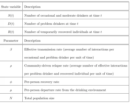
Table 1: State variables and parameters of the contagion model in well-mixed drinking communities.
State variable Description
S(t) Number of occasional and moderate drinkers at timet D(t) Number of problem drinkers at time t
R(t) Number of temporarily recovered individuals at timet
Parameter Description
β Effective transmission rate (average number of interactions per
occasional and problem drinker per unit of time)
ρ Community-driven relapse rate (average number of effective interactions
per problem drinker and recovered individual per unit of time)
φ Per-person recovery rate
the partial derivatives in equation (6). Before we outline this computation we introduce some notation. The vector
θ= (N, µ, β, ρ, φ),
denotes the model parameters. On the other hand, u(t;θ) = (S(t;θ), D(t;θ), R(t;θ))T
denotes the state variable vector, at timetfor a givenθ. We also assumeg= (g1, g2, g3) is the vector function whose entries are given by the expressions on the right sides of equations (1)–(3), and write
du
dt =g(u(t;θ);θ). (7)
Since the function g is differentiable, taking the partial derivatives ∂/∂θ of both sides
of equation (7) we obtain the differential equation
d dt ∂u ∂θ = ∂g ∂u ∂u ∂θ + ∂g
∂θ. (8)
In equation (8) the 3×3 matrix ∂g/∂uis equal to
−$Nβ +µ% −NβS 0
β
ND
β
NS+
ρ
NR−(µ+φ)
ρ
ND
0 φ− NρR −&NρD+µ'
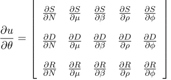
while∂u/∂θ is a 3×5 matrix given by ∂u ∂θ = ∂S
∂N ∂S∂µ ∂S∂β ∂S∂ρ ∂S∂φ
∂D
∂N ∂D∂µ ∂D∂β ∂D∂ρ ∂D∂φ
∂R
∂N ∂R∂µ ∂R∂β ∂R∂ρ ∂R∂φ
.
Numerical values of∂u/∂θ are calculated by solving (7) and (8) simultaneously; we define
x(t) = ∂u∂θ(t;θ), let the parameters be evaluated at some known values, θ = ˆθ, and solve
the following differential equations fromt=t0 tot=tn,
du
dt = g(u(t;θ);θ) (9)
d
dtx(t) =
∂g
∂ux(t) +
∂g
∂θ (10)
x(0) = 0. (11)
Relative sensitivity functions, sφ(t) and sρ(t), defined as
sφ(t) =
φ D(t; ˆθ)
∂D
∂φ(t; ˆθ) (12)
sρ(t) =
ρ D(t; ˆθ)
∂D
∂ρ(t; ˆθ), (13)
are dimensionless variables, that can be used to compare, within the same scale, the degree of sensitivity ofD(t) with respect to the recovery rate φand the relapse rateρ.
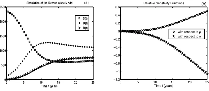
Figure 1 displays numerical solutions to equations (9)–(10), obtained while using known parameter values suggested in [15] (the units are written in square brackets); N = 2500;
1(a), the number of, at timet: occasional and moderate drinkers, S(t), problem drinkers,
D(t), and temporarily recovered individuals, R(t), are shown in squares, crosses, and
tri-angles, respectively. Figure 1(b) displays the relative sensitivity functions; sφ(t)(stars)
and sρ(t) (circles), versus timet. Neither of these functions changes sign, during the time
window under consideration, suggesting monotonic behavior in D(t) originates from
fluc-tuations in the parameters. On one hand, it is seen the functionsρ(t) is positive (sρ(t)>0
for 0 < t < 25), implying that the number of problem drinkers, D(t), is increasing
rela-tive to increments in the relapse rate ρ. On the other hand, sφ(t) < 0 for 0 < t < 25,
suggests that variations in the recovery rateφ, cause the number of problem drinkers to
0 5 10 15 20 25 0 500 1000 1500 2000 2500
Time t [years] Simulation of the D eterministic M odel
S(t) D (t) R (t)
(a)
! " #! #" $! $"
!#%$ !# !!%& !!%' !!%( !!%$ ! !%$ !%( !%' )*+,-.-/0,1234 5,61.*7,-8,93.*7*.0-:;9<.*=93 ->*.?-2,3@,<.-.=-! >*.?-2,3@,<.-.=-" ABC
Figure 1: Numerical solutions of the deterministic model for drinking dynamics. Panel (a) shows S(t) (squares), D(t) (crosses), and R(t) (triangles), as functions of time t,
respec-tively. Panel (b) displays the relative sensitivity functions, ρ
D(t)
∂D(t)
∂ρ (circles) and φ
D(t)
∂D(t)
∂φ
(stars), versus time t. The baseline values used to obtain these numerical solutions are:
3
A Stochastic Model in Well-mixed Drinking Communities
In this Section we derive a stochastic model from the deterministic formulation described by equations (1)–(4). The goal is to quantify the variability on drinking dynamics due to stochastic effects; intending to highlight some of the differences and similarities between the deterministic and stochastic approaches.
The derivation of the stochastic model is standard —see for instance[28, 29]— and our analysis here is primarily based on simulations. Transitions between drinking classes involve discrete events which change the number of individuals in every class, one at a time. For example, when a drinking contagion event occurs, the number of moderate drinkers is decreased by one, while the number of problem drinkers increases by one. The probability an event takes place during an infinitesimal time interval [t, t+dt] is calculated from the
average rates in the deterministic model (the probability equals the rate multiplied by the length of the time interval). In the example mentioned above, the event occurs at a rate equal toβS(t)D(t)/N, then the probability it happens during [t, t+dt] is (βS(t)D(t)/N)dt.
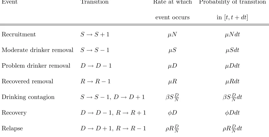
All the events, their rates of occurrence, and the probabilities at which they take place are listed in Table 2.
It is assumed the events (see first column in Table 2) are described by independent Poisson processes [28]. The term
E=µN+µS+µD+µR+βSD/N+φD+ρRD/N, (14)
Table 2: Possible events in the drinking model, their rates and probabilities of their occur-rence in time interval [t, t+dt]. For simplicity, the dependence ont is omitted, writingS,
D, and R, instead ofS(t), D(t), andR(t), respectively.
Event Transition Rate at which Probability of transition event occurs in [t, t+dt]
Recruitment S →S+ 1 µN µN dt
Moderate drinker removal S →S−1 µS µSdt
Problem drinker removal D→D−1 µD µDdt
Recovered removal R→R−1 µR µRdt
Drinking contagion S →S−1,D→D+ 1 βSDN βSDNdt
Recovery D→D−1,R→R+ 1 φD φDdt
dependence on t and we writeS, D, and R, instead of S(t),D(t), and R(t), respectively.
The time between events is exponentially distributed with mean 1/E; in fact, the time at
which the next event happens is found by sampling from an exponential distribution with mean 1/E.
To decide which event takes place (once it is known an event occurs), we divide up the interval (0, E) into lengths that correspond to the relative occurrence probabilities of the
various events. In other words, given that an event has occurred, the probability that it is a recruitment is µN/E, the probability that it is a moderate drinker removal is µS/E,
the probability that it is a problem drinker removal is µD/E, etc. A random number U
is sampled from the uniform distribution on (0,1) and an event is selected if this sampled
number falls within the subinterval in (0, E) corresponding to such event. For instance,
we decide that a recruitment has occurred if 0< U < µN/E, a moderate drinker removal
ifU lies between µN/E and (µN+µS)/E, a problem drinker removal if U lies between
(µN+µS)/E and (µN+µS+µD)/E, and so on.
The average behavior of the stochastic model described in Table 2 is compared to its deterministic analog when stochastic realizations and numerical solutions are computed using the same parameter values (N = 2500; β= 0.65;ρ= 0.10;φ= 0.10; andµ= 0.10).
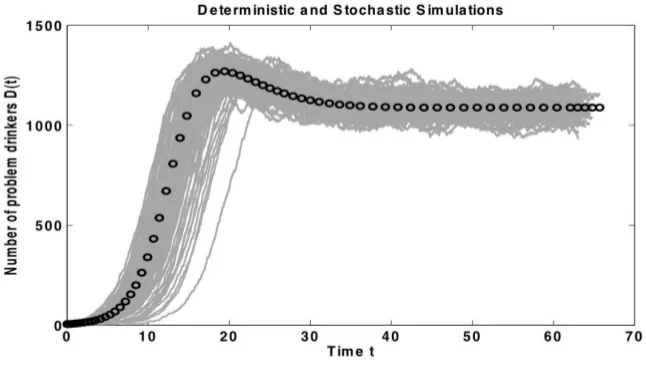
In Figure 2 it is observed the dynamics of the deterministic model (black circles) agrees with the mean (over 100 realizations) dynamics of the stochastic model (grey curves), as is expected whenRφ>1 (albeit extinction in the stochastic model is theoretically possible;
Figure 2: Results from numerical simulations. 100 stochastic realizations (grey curves) and numerical solutions of the deterministic (black circles) problem drinker class D(t) versus
time t. For these simulations the following values of parameters were used: N = 2500;
and the stochastic model (Table 2) is that for the same set of parameters: the latter model gives rise to several distinct time trajectories, each of them referred to as a realization, while the former model gives an only possible outcome. The variability of the number of problem drinkers, at a particular time point, can be quantified from the realizations of the simulated stochastic model. For instance, letting T denote a stoppage time (if tj
denotes the time at which thejth event takes place, see equation (14), then define T =tn,
for some n, as the stoppage time of the simulations —for those displayed in this Section,
we used n = 10000), then the variability of D(T) can be quantified by calculating its
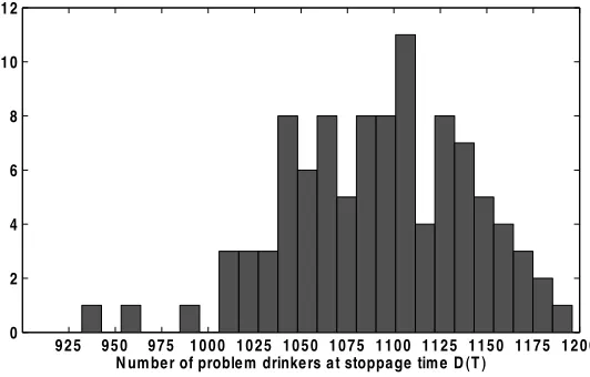
mean and variance from the realizations. To illustrate the variability ofD(T) (number of
problem drinkers at a stoppage time T) we show a histogram in Figure 3, resulting from
100 stochastic realizations.
It is of interest to investigate how the stochastic drinking dynamics are affected by the recovery and relapse rates. We address it using simple numerical experiments, which quantify the dependence of D(T) on ρ (relapse rate) and φ (recovery rate assumed to be
fueled by treatment). More precisely, most of the model parameters are held fixed while one parameter is varied, and 25 realizations of the stochastic model are calculated: φis varied
fromφ= 1.0×10⁻⁸ toφ= 5.0×10⁻¹;ρ is varied from ρ= 1.0×10⁻⁸ toρ= 5.0×10⁻¹;
while N = 2500; β = 0.65; ρ = 0.10 (while varying φ); φ = 0.10 (while varying ρ); and
µ = 0.10. Figure 4(a) displays the mean and standard deviation of D(T) versus φ; the
9 2 5 9 5 0 9 7 5 1 0 0 0 1 0 2 5 1 0 5 0 1 0 7 5 1 1 0 0 1 1 2 5 1 1 5 0 1 1 7 5 1 2 0 0 0
2 4 6 8 1 0 1 2
N um be r of proble m drinke rs a t stoppa ge tim e D (T )
Figure 3: Histogram of D(T), number of problem drinkers at stoppage time T, resulting
from 100 stochastic realizations.
lower dashed curve. It is seen that the meanD(T) decreases as a function of the recovery
rateφ, this is consistent with the information conveyed by the relative sensitivity function
sφ(t) in Figure 1(b). On the other hand, Figure 4(b) displays the meanD(T), and the mean D(T) plus (upper dashed curve) and minus (lower dashed curve) one standard deviation,
as functions ofρ. It is clear the meanD(T) is an increasing function of the relapse rateρ,
0 0.1 0.2 0.3 0.4 0.5 0
500 1000 1500 2000 2500
R ecovery rate !
D
(T
)
(a)
0 0 .1 0 .2 0 .3 0 .4 0 .5
8 0 0 1 0 0 0 1 2 0 0 1 4 0 0 1 6 0 0 1 8 0 0 2 0 0 0
R e la pse ra te !
D
(T
)
(b)
Figure 4: Results from 25 stochastic simulations while varying the recovery rateφand the
relapse rateρ. Panel (a) displays the mean number (solid square) of problem drinkers at a
stoppage time T,D(T), along with the mean plus/minus one standard deviation (dashed
curves), for each value ofφused in the simulations; from φ= 1.0×10⁻⁸ toφ= 5.0×10⁻¹. Panel (b) shows the meanD(T), and the mean plus (upper dashed curve) and minus (lower
dashed curve) one standard deviation, versusρ; fromρ= 1.0×10⁻⁸ toρ= 5.0×10⁻¹. The other parameters were held fixed at the following values: N = 2500; β = 0.65; ρ = 0.10
4
A Stochastic Model for Structured (Small-world)
Drink-ing Communities
The fact that several processes (including drinking) are highly dependent on the contacts and types of contacts between heterogeneous individuals has motivated the study of epi-demics on networks [30, 31, 32]. A network (graph) is a set of nodes and connections between them (edges). Random graphs are natural representations of the space (land-scape) of contacts between individuals in a population; by letting each node represent an individual and allowing a random connection between two nodes resemble a potential contact [33].
Watts and Strogatz [34] introduced a parametrization of families of networks that inter-polate between two architectures (topologies): from a regular lattice to a random graph. Their proposed parametrization is stated as an algorithm (used to construct networks) which is initialized with a one-dimensional periodic ring lattice ofN nodes, each of them
connected to the closest &k' neighbors (two nodes are neighbors if there is an edge
con-necting them). The network continues to be updated by re-wiring each edge to a randomly selected node with probabilityp(referred to as the disorder parameter). When the disorder
parameter satisfiesp→0, then the algorithm leaves the lattice intact, whilep→1 implies
transmis-sion. This property is known as the small-world effect and was discovered by the social psychologist S. Milgram as a result of letter-forwarding experiments [36]. In addition, these networks (constructed with the Watts-Strogatz algorithm) have also a property called clus-tering, which pertains to how the neighborhoods of connected nodes overlap (cliquishness), in other words, whether or not “friends of friends are friends of each other” [34].
In this study we use the terms network and community interchangeably. Moreover, community structure is modeled by random graphs; with nodes representing individuals and random edges denoting social connections to other individuals which may lead to a conversion into a problem drinker. Nodes can be in one of three distinct states: moderate drinkers, problem drinkers, and temporarily recovered. They transition between states according to probabilities which are functions of time and the number of neighbors in particular states. Suppose there is a community with N nodes; a given node i (where
1 ≤ i≤ N) has δ(i, t) neighbors who, at time t, are in the state called problem drinker.
We define the probability nodeichanges:
1. from moderate drinker into problem drinker as 1−exp(−βδ(i, t)), where β denotes
the transmission rate;
2. from problem drinker into temporarily recovered as 1−exp(−φ), where φ denotes
the recovery rate;
3. from temporarily recovered into problem drinker as 1−exp(−ρτ(t)δ(i, t)), whereρτ(t)
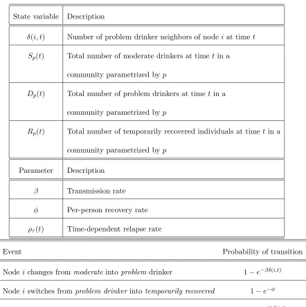
Table 3: State variables, parameters, events, and transition probabilities of the drinking contagion model in small-world communities.
State variable Description
δ(i, t) Number of problem drinker neighbors of nodeiat time t
Sp(t) Total number of moderate drinkers at timet in a
community parametrized byp
Dp(t) Total number of problem drinkers at time tin a
community parametrized byp
Rp(t) Total number of temporarily recovered individuals at time tin a
community parametrized byp
Parameter Description
β Transmission rate
φ Per-person recovery rate ρτ(t) Time-dependent relapse rate
Event Probability of transition
Nodeichanges from moderateinto problemdrinker 1−e−βδ(i,t) Nodeiswitches fromproblem drinker intotemporarily recovered 1−e−φ
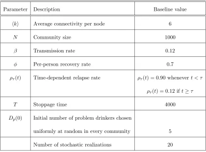
Table 4: Parameter values utilized in simulations of drinking contagion in small-world communities.
Parameter Description Baseline value
&k' Average connectivity per node 6
N Community size 1000
β Transmission rate 0.12
φ Per-person recovery rate 0.7
ρτ(t) Time-dependent relapse rate ρτ(t) = 0.90 whenevert < τ ρτ(t) = 0.12 if t≥τ
T Stoppage time 4000
Dp(0) Initial number of problem drinkers chosen
This formulation (see Table 3) determines a stochastic process and the terms Sp(t),
Dp(t), and Rp(t) are random variables denoting, at time t, the total number of
moder-ate drinkers, problem drinkers, and temporarily recovered, respectively, in a community parametrized by the disorder parameterp.
We simulate drinking dynamics among small-world communities, by calculating stochas-tic realizations of the random networks [34] and the stochasstochas-tic process defined in Table 3, while using the parameter baseline values summarized in Table 4. We relax the assumption about time between events being exponentially distributed; instead we let time between events have length one, with arbitrary time units.
To contrast the role played by a time-dependent relapse rate, we consider bothρτ(t)≡0
and ρτ(t) *= 0. In the case ρτ(t) ≡0 —that is, assuming nobody relapses after drinking
stops— the model reduces to a network SIR epidemic model [31] with a well known qualita-tive behavior; the number of problem drinkers grows from a small number until it peaks at a maximum to later fade out, since eventually everyone recovers. This feature derives from the deterministic [23] and stochastic [28] single-outbreak SIR model, only being enhanced by the community structure.
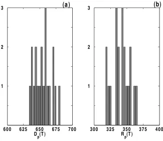
Histograms of Dp(T) andRp(T), whereT denotes a stoppage time in the simulations
(see Table 4), are computed for each value of p; for instance, Figure 5 displays the
his-tograms obtained over 20 realizations withp= 3.02×10⁻⁴. To assess the role community
6(a) shows that Dp(T) = 0, for all p, implying that every problem drinker node
eventu-ally becomes temporarily recovered across all community structures. However, the average size, at a stoppage time T, of the temporarily recovered class Rp(T), displayed in
Fig-ure 6(b), varies substantially for various community structFig-ures; random networks with
1.00×10⁻⁴ < p <1.00×10⁻² have mean Rp(T) values under 200 (less than 20%), while
communities with 1.00×10⁻¹ < p <1.00 display averageRp(T) values between 600 and
800 (from 60% to 80%). The results of Figure 6(b) suggest that in the absence of demo-graphics and relapse, the community structure does affect the total number of temporarily recovered individuals; small average distance between nodes (in the community) promotes drinking contagion.
The next case considered here uses a nontrivial time-dependent relapse rate,ρτ(t)*= 0,
defined as
ρτ(t) =
0.90 ift < τ
0.12 ift≥τ,
(15)
whereτ denotes a time at which the relapse rate drops as a result of treatment. The values
of the relapse rate were chosen to have the average relapse probability change, at t = τ,
from
1−e−ρτ(t)#k$≈1 (16)
to
1−e−ρτ(t)#k$≈0.50, (17)
600 625 650 675 700 1
2 3
D
p(T )
300 325 350 375 400
1 2 3
R
p(T )
(a)
(b)
Figure 5: Histograms of the total number of problem drinkers and temporarily recovered individuals,Dp(T) and Rp(T), respectively, at a stoppage time T. Samples obtained from
20 stochastic realizations in simulated communities withp = 3.02×10⁻⁴ (the parameter
1 0!4 1 0!3 1 0!2 1 0!1 1 00
!1
!0 .5 0 0 .5 1
M
e
a
n
D p
(T
)
1 0!4 1 0!3 1 0!2 1 0!1 1 00
0 2 0 0 4 0 0 6 0 0 8 0 0 1 0 0 0
M
e
a
n
R p
(T
)
N e twork disorde r pa ra m e te r p
(b)
(a )
Figure 6: Average and variance ofDp(T) andRp(T) as functions of the simulated
commu-nity architecture parametrized byp(logarithmic scale). The mean (circles) and mean plus
and minus one standard deviation (dash curves) are computed from 20 stochastic realiza-tions for each fixed value ofp. Panels (a) and (b) display results of simulated contagion in
p = 0 (see Table 4; for the simulations we set &k' = 6). The average relapse probability
of equation (16) illustrates a worst-case scenario in which temporarily recovered nodes become problem drinkers with probability nearly one. Figure 7 displays results for a worst-case scenario using τ = ∞ (i.e. the relapse rate remains constant). Under this
scenario we find community structure does not affect the average size of either the problem drinker or the temporarily recovered class; all communities seem to be equally at risk of supporting endemic levels of problem drinkers (these levels are above 60%, 600 out 1000, of the community size). It is seen in Figure 7 that on average Dp(T) +Rp(T) = 1000;
implying that every node in the simulated communities has been converted into a problem drinker at least once, leaving the total number of moderate drinkers nearly empty.
The sensitivity of the prevalence levels of problem drinkers, at time T, with respect
to the recovery and relapse rates is investigated by simulating drinking dynamics, while increasing the values ofφandρ, respectively. More precisely: the recovery rate is increased
from φ= 1.0×10⁻⁴ to φ= 3.0×10⁻¹; the relapse rate is increased from ρ = 1.0×10⁻¹
to ρ = 2.5; while all the other parameters are held fixed at values displayed in Table
4. It can be observed in Figure 8(a) that when displayed as a function of the recovery rate φ, the mean Dp(T) decreases to nearly one-half, for p = 0 and p = 1, respectively.
Hence, increasing the recovery rate when the average relapse probability is extremely high (1−e−ρτ(t)#k$ ≈1) promotes reductions in the number of problem drinkers (and therefore
1 0!4 1 0!3 1 0!2 1 0!1 1 00 4 0 0
5 0 0 6 0 0 7 0 0 8 0 0
M e a n D p (T )
1 0!4 1 0!3 1 0!2 1 0!1 1 00
2 0 0 2 5 0 3 0 0 3 5 0 4 0 0 4 5 0
M e a n R p (T )
N e twork disorde r pa ra m e te r p
(b)
(a )
Figure 7: Dependence of the average and variance ofDp(T) andRp(T) on the community
structurep(logarithmic scale). Average (circles) and one standard deviation added to and
subtracted from the average (dash curves) are calculated from 20 stochastic realizations for each fixed value of p. The results shown in Panels (a) and (b) assess a “worst case
as ρ increases the average Dp(T) increases as well. Network structure does not affect
the sensitivity of φ, however, it does affect the sensitivity of ρ: Figure 8(b) suggests that
small average distance between nodes, in the drinking community, results in larger average numbers of problem drinkers —compare the mean Dp(T) at p = 1 (circles) and p = 0
(squares) for 0.10< ρ< 0.25.
The sensitivity of the meanDp(T) with respect to the relapse rate, Figure 8(b), suggests
that while using a time-dependent relapse rate ρτ(t), with τ < ∞, one would expect
significant outcomes. To explore numerically the role of applying successful treatment programs in drinking communities, which prevent temporarily recovered individuals from relapse, at distinct timesτ, we carry out simulations forτ = 3, 5, 7, 10. Figure 9 displays
the effect of how long it takes to launch treatment programs that reduce relapse; it suggests that for τ = 3, 5, 7, 10, there is not much differences in the average Dp(T) and Rp(T).
However, these averages give evidence of improvement when compared to those obtained withτ =∞. Therefore, the treatment programs promoting a lower relapse are beneficial,
0 0.25 0.5 0.75 1 1.25 1.5 1.75 2 2.25 2.5 0 200 400 600 800 1000
R ecovery rate !
M e a n D p (T ) p=0 p=1 (a)
0 0.05 0.1 0.15 0.2 0.25 0.3 0 100 200 300 400 500 600 700 800 900 1000
R elapse rate !
M e a n D p (T ) p=0 p=1 (b)
Figure 8: Dependence of the averageDp(T) on the recovery rate,φ, and the relapse rate,ρ.
The averages of 10 stochastic realizations are displayed for simulated communities obtained atp = 0 (squares) and p = 1 (circles). Panels (a) and (b) provide basic measures on the
sensitivity of the meanDp(T) to variations in φand ρ, respectively. It is clear from Panel
(a) that increments in the recovery rateφlead to a decay in the mean Dp(T); while Panel
(b) suggests that a decay in the meanDp(T) is expected from decreasing the relapse rate
ρ. It is seen in Panel (b) that simulated communities obtained at p = 1 (circles) seem
to accumulate larger numbers of problem drinker nodes relative to those of communities with p= 0, for 0.10 < ρ < 0.25. On the other hand, Panel (a) shows that both types of
community structure (p= 0 andp= 1) have the same decreasing behavior inDp(T) as φ
!"!# !"!$ !"!% !"!! !"" " !"" %"" $"" #"" &"" '"" ("" )*+,-./0123-.1*.045.56*+*.04 7*5809 4 :;< 0 0 !=$ !=& !=( !=!" !="
!"!# !"!$ !"!% !"!! !""
" !"" %"" $"" #"" &"" '"" ("" >"" ?"" !""" )*+,-./0123-.1*.045.56*+*.04 7*580@ 4 :;< 0 0 !=$ !=& !=( !=!" !=" :5< :A<
Figure 9: AverageDp(T) andRp(T) as functions of the community structure parameterized
byp. Panels (a) and (b) display the results obtained from using a time-dependent relapse
rate ρτ(t). The relapse rate is decreased from 0.90 to 0.12 at time t = τ. In this way
on average every node diminishes its probability to change from temporarily recovered into problem drinker by half. In symbols, the probability 1−e−0.90#k$ ≈ 1 decreases to
1−e−0.12#k$≈0.5. Panels (a) and (b) show the averages sampled by applying this relapse reduction at distinct times: τ = 3 (upward triangles); τ = 5 (diamonds); τ = 7 (right
triangles); τ = 10 (circles). The averages displayed in Figure 7 are shown here as τ =∞
5
Discussion
Under the assumption of homogeneous mixing we model drinking dynamics as a contact process [15, 39]; using a simple deterministic formulation based on nonlinear differential equations. The sensitivity equations of the deterministic model are derived and numerical solutions, obtained using known parameter values, are suggestive of the roles played by the relapse and recovery rates in the prevalence of problem drinkers. The numerical solutions displayed in Figure 1(b) suggest the establishment of problem drinkers would benefit from increments in the relapse rate, while increasing recovery rates should be detrimental for such establishment.
The deterministic model, introduced in Section 2, is extended into a stochastic model; by allowing the contact process to evolve according to stochastic rules. This stochastic formulation permits to quantify the variability in the size of the problem drinker class and using numerical studies we confirm that: (i) the deterministic model matches the average behavior of the stochastic model; (ii) the meanD(T) decreases as a function of the recovery
rateφ; and is an increasing function of the relapse rate ρ.
algorithm [34] and are parameterized by a disorder parameter p. For p = 0, we have a
situation where individuals only interact locally, that is, only with the nearest neighbors, while when p = 1 they basically interact with everybody in the community. According
to the simulations under a worst-case scenario —having a high average relapse probabil-ity, 1−e−ρτ(t)#k$ ≈ 1, with τ = ∞— all community structures are equally exposed to
develop nearly the same average endemic levels of problem drinkers. On the other hand, improvements (reductions in mean Dp(T)) are seen when simulating treatment programs
that promote lowering the relapse rate at various times (τ = 3,5,7,10); network structure
plays a role in the latter scenario, the meanDp(T) and Rp(T) attain higher levels asp→1
(see Figure 9).
6
Acknowledgments
A. C.-A. was also supported in part by Grant Number R01AI071915-07 from the National Institute of Allergy and Infectious Diseases. The content is solely the responsibility of the authors and does not necessarily represent the official views of the NIAID or the NIH.
References
[1] National Institute of Alcohol Abuse and Alcoholism, NIAAA five year strategic plan, website:
http://pubs.niaaa.nih.gov/publications/StrategicPlan/NIAAASTRATEGICPLAN.htm, accessed on April 29, 2008.
[2] Centers for Disease Control and Prevention, Alcohol and public health, website: http://www.cdc.gov/alcohol/index.htm, accessed on April 29, 2008.
[3] Leadership to keep children alcohol free, website: http://www.alcoholfreechildren.org/, accessed on May 11, 2008.
[4] College drinking, website: http://www.collegedrinkingprevention.gov/, accessed on May 11, 2008.
http://www.cdc.gov/alcohol/quickstats/general info.htm, accessed on May 1, 2008.
[6] National Institute of Alcohol Abuse and Alcoholism, frequently asked questions for the general public, website:
http://www.niaaa.nih.gov/FAQs/General-English/default.htm, accessed on April 29, 2008.
[7] K. Daido, Risk-averse agents with peer pressure.Appl. Econ. Lett.11, 383-386 (2004).
[8] E. R. Weitzman, A. Folkman, K. L. Folkman, and H. Weschler, The relationship of alcohol outlet density to heavy and frequent drinking and drinking-related problems among college students at eight universities. Health Place9, 1-6 (2003).
[9] A. Mubayi, P. Greenwood, C. Castillo-Ch´avez, P. Gruenewald, and D. M. Gorman, On the impact of Relative Residence Times, in Highly Distinct Environments, on the Distribution of Heavy Drinkers.Socio. Econ. Plan. Sci. (In press, 2008).
[10] C. Castillo-Chavez, W. Huang, and J. Li, Competitive Exclusion in Gonorrhea Models and Other Sexually-Transmitted Diseases.SIAM J. Appl. Math. 56, 494-508 (1996).
[12] G. Chowell, C. E. Ammon, N. W. Hengartner, J. M. Hyman, Transmission dynamics of the great influenza pandemic of 1918 in Geneva, Switzerland: Assessing the effects of hypothetical interventions. J. Theor. Biol.241, 193-204 (2006).
[13] C. Castillo-Ch´avez, J. X. Velasco-Hern´andez, and S. Fridman, Modeling contact struc-tures in biology, InFrontiers of Theoretical Biology. Lecture Notes in Biomathematics, Vol. 100(Edited by S. A. Levinet al.), pp. 454-491. Springer-Verlag. New York (1994).
[14] O. Diekmann and J. A. P. Heesterbeek,Mathematical Epidemiology of Infectious Dis-eases: Model Building, Analysis and Interpretation, Wiley, Chichester, New York (2000).
[15] F. Sanchez, X. Wang, C. Castillo-Chavez, D. M. Gorman, P. J. Gruenewald, Drinking as an epidemic—a simple mathematical model with recovery and relapse. In Thera-pist’s Guide to Evidence-Based Relapse Prevention: Practical Resources for the Mental
Health Professional, (Edited by K. A. Witkiewitz and G. A. Marlatt), pp. 353-368. Academic Press, Burlington, Massachusetts (2007).
[16] L. M. A. Bettencourt, A. Cintr´on-Arias, D. I. Kaiser, and C. Castillo-Ch´avez, The power of a good idea: quantitative modeling of the spread of ideas from epidemiological models. Physica A 364, 513-536 (2006).
[18] S. B. Patten, and J. A. Arboleda-Florez, Epidemic theory and group violence. Soc. Psych. Psych. Epid. 39, 853-856 (2004).
[19] M. Gladwell, The Tipping Point.New Yorker72, 32-39 (1996).
[20] B. Song, M. Castillo-Garsow, C. Castillo-Ch´avez, K. R´ıos Soto, M. Mejran, and L. Henso, Raves, Clubs, and Ecstasy: The Impact of Peer Pressure. Math. Biosci. Eng.
3, 249-266 (2006).
[21] D. R. Mackintosh, and G.T. Stewart, A mathematical model of a heroin epidemic: implications for control policies. J. Epidemiol. Commun. H.33, 299-304 (1979).
[22] R. J. Braun, R. A. Wilson, J. A. Pelesko, and J. R. Buchanan, Applications of small-world network theory in alcohol epidemiology.J. Stud. Alcohol 67, 591-599 (2006).
[23] F. Brauer, and C. Castillo-Ch´avez, Mathematical Models in Population Biology and Epidemiology, Texts in Applied Mathematics 40, Springer-Verlag, New York (2001).
[24] Centers for Disease Control and Prevention, Frequently Asked Questions; what does moderate drinking mean?, website: http://www.cdc.gov/alcohol/faqs.htm#6, ac-cessed on May 11, 2008.
[26] P. Bai, H. T. Banks, S. Dediu, A. Y. Govan, M. Last, A. L. Lloyd, H. K. Nguyen, M. S. Olufsen, G. Rempala, and B. D. Slenning, Stochastic and deterministic models for agricultural production networks. Math. Biosci. Eng.4, 373-402 (2007).
[27] M. Eslami, Theory of Sensitivity in Dynamic Systems: An Introduction, Springer-Verlag, New York, New York (1994).
[28] L. J. S Allen, An Introduction to Stochastic Processes with Applications to Biology, Pearson Education-Prentice Hall, Upper Saddle River, New Jersey (2003).
[29] E. Renshaw, Modelling Biological Populations in Space and Time, Cambridge Univ. Press, Cambridge, New York (1991).
[30] A. L. Lloyd, and R.M. May, Epidemiology. How viruses spread among computers and people. Science292, 1316 (2001).
[31] L. A. Meyers, Contact network epidemiology: bond percolation applied to infectious disease prediction and control. B. Am. Math. Soc. 44, 63-86 (2007).
[32] R. Pastor-Satorras, and A. Vespignani, Epidemic spreading in scale-free networks.
Phys. Rev. Lett. 86, 3200 (2001).
[34] D. J. Watts, and S. H. Strogatz, Collective dynamics of ‘small-world’ networks.Nature
383, 440-442 (1998).
[35] B. Bollob´as,Random Graphs, Cambridge Univ. Press, Cambridge, New York (2001).
[36] S. Milgram, The small world problem.Psychol. Today1, 60-67 (1967).
[37] G. Chowell, and C. Castillo-Ch´avez, Worst-case scenarios and epidemics, In Bioterror-ism: Mathematical Modeling Applications in Homeland Security. Frontiers in Applied
Mathematics vol. 28., (Edited by H. T. Banks and C. Castillo-Ch´avez), pp. 35-53. Society for Industrial and Applied Mathematics. Philadelphia, Pennsylvania (2003).
[38] G. Chowell, A. Cintr´on-Arias, S. Del Valle, F. S´anchez, B. Song, J. M. Hyman, H. W. Hethcote, and C. Castillo-Ch´avez, Mathematical applications associated with the deliberate release of infectious agents, In Modeling the Dynamics of Human Disease: Emerging Paradigms and Challenges. Contemporary Mathematics Series vol. 410. , (Edited by A. Gummelet al.), pp. 51-72. American Mathematical Society. Providence, Rhode Island (2006).
[39] J. Orford, M. Krishnan, M. Balaam, M. Everitt, and K. Van der Graaf, University student drinking: the role of motivational and social factors.Drug-Educ. Prev. Polic.