ABSTRACT
RICE, JENNA MARIE. Teachers’ Use of Technology in Solving an Informal Inference Problem. (Under the direction of Dr. Hollylynne Stohl Lee.)
Informal statistical inference is the process of making inferences based on data without using formal statistical procedures. The purpose of this study is to examine how teachers use technology to solve an informal inference problem, and to determine their levels of reasoning about the relationship between expectation, variation, and sample size.
Fifty-seven pre-service and in-service teachers across three institutions in the United States wrote documents describing their problem-solving strategies for a specific task. These documents ranged in length from one page (including screenshots) to fifteen pages. This study utilized a case study approach that considered three different technologies, Probability Explorer, Microsoft Excel, and Fathom, to be three cases.
A framework to determine teachers’ levels of reasoning about the relationship
between expectation, variation, and sample size was modified from the framework described by Watson, Callingham, and Kelly (2007). The modified framework outlined hierarchical levels of reasoning that ranged from Inconsistent to Explanatory Comparative. Teachers were coded at specific levels based on their responses and how they used simulated data to support their conclusions.
The findings from this study indicate that teachers who use Probability Explorer tend to simulate fewer repeated samples than teachers who use Microsoft Excel or Fathom,
Teachers’ Use of Technology in Solving an Informal Inference Problem
by
Jenna Marie Rice
A thesis submitted to the Graduate Faculty of North Carolina State University
in partial fulfillment of the requirements for the degree of
Master of Science
Mathematics Education
Raleigh, North Carolina 2013
APPROVED BY:
_______________________________ ______________________________
Dr. Herle McGowan Dr. Allison W. McCulloch
BIOGRAPHY
Jenna Rice was born and raised in New Bern, North Carolina. She is the daughter of Frank and Kathleen Rice, and the younger sister of Jeff. Jenna graduated from New Bern High School in 2007 with honors, and went on to attend North Carolina State University for her undergraduate career. She graduated summa cum laude from N. C. State in 2011 with a B.S. in Mathematics Education and a B.S. in Statistics. After participating in research opportunities as an undergraduate in both statistics and mathematics education, Jenna decided to pursue an M.S. in Mathematics Education and began her graduate career during the summer of 2011.
Jenna currently teaches at Lee Early College High School in Sanford, NC. She has taught high school math there for one and a half years. Jenna has taught Geometry, Algebra 2, Advanced Functions and Modeling, and she is excited to teach Statistics this year. She enjoys teaching at LEC because of her wonderful colleagues and her clever and funny students.
ACKNOWLEDGMENTS
I would like to thank all of the teachers I have had the privilege of learning from throughout my life. From Pre-K to graduate school, my teachers have been invaluable in my growth as a life-long learner. Thank you for instilling confidence in my mathematical
abilities, and for pushing me to be a better writer. Thank you for showing me the joy of learning, and that perseverance is the key to success. Thank you for the years of service you have committed to your community. Thank you. I hope to pay it forward.
I would like to express my gratitude to my advisor, Dr. Hollylynne Stohl Lee for her support and guidance throughout this process. The ability to bounce ideas off of someone who is so knowledgeable and to ask for advice or suggestions has been priceless. Also, I would like to thank Dr. McCulloch and Dr. McGowan for their suggestions and patience during this project, and for their willingness to serve as committee members.
I would also like to thank my family for believing in me, and for supporting me in my endeavors. Thank you for caring about my success in school without demanding
unachievable perfection. I feel lucky to have a family so supportive of my ambitions, even when they seem to come out of nowhere. To my brother, Jeff, thank you for motivating me to reach the high bar you set before me.
For my friends who are teachers, thank you for working hard and making a
The research reported in this thesis was partially supported by the National Science Foundation under Grant Nos. DUE 0442319 and DUE 0817253 awarded to North Carolina State University. Any opinions, findings, and conclusions or recommendations expressed herein are those of the author and do not necessarily reflect the views of the National Science Foundation. The researcher also thanks the mathematics teacher education faculty and
TABLE OF CONTENTS
LIST OF TABLES ... ix
LIST OF FIGURES ...x
CHAPTER 1: INTRODUCTION ...1
Statement of the Problem ...5
CHAPTER 2: LITERATURE REVIEW ...6
Informal Statistical Inference ...6
Frameworks for Informal Statistical Inference ...7
Samples ...8
Sample Size ...9
Sampling Variation ...12
Sampling Variation with Respect to Expectation ...14
Sampling Distributions ...16
Sample Collection ...19
Simulations ...20
Probability Explorer ...22
Fathom ...25
Microsoft Excel ...28
Graphing Calculator ...30
The Teacher’s Role ...31
CHAPTER 3: METHODOLOGY ...35
Larger Study...35
Context for the Study ...36
Analysis Techniques ...38
Coding Initial Expectations for the Proportion ...39
Coding Variation with Respect to Sample Size ...41
Coding Repeated Sampling...44
Formation of Conclusions ...46
Looking Across Cases...53
CHAPTER 4: RESULTS BY TECHNOLOGY CASE ...55
Probability Explorer ...55
Reasons for Choosing Probability Explorer ...56
Initial Expectations for the Proportion of Hats ...57
Reasoning About Variation with Respect to Sample Size ...59
Engaging in Repeated Sampling ...60
Use of Probability Explorer to Formulate Conclusions ...62
Microsoft Excel ...64
Reasons for Choosing Microsoft Excel ...64
Initial Expectations for the Proportion of Hats ...66
Reasoning About Variation with Respect to Sample Size ...67
Use of Excel to Formulate Conclusions ...70
Fathom ...72
Reasons for Choosing Fathom ...72
Initial Expectations for the Proportion of Hats ...74
Reasoning About Variation with Respect to Sample Size ...75
Engaging in Repeated Sampling and Forming Conclusions ...76
Comparing the Cases ...77
Reasoning Levels in Parts (a) and (b) ...78
Comparing Repeated Sampling for Technology ...78
Comparing Conclusion Types for Technology ...79
Choosing a Technology ...80
CHAPTER 5: RESULTS BY CROSS-CASE ANALYSIS ...82
Type of Sampler vs. Variation with Respect to Sample Size ...82
Type of Sampler vs. Type of Conclusion ...85
Comparing Levels of Reasoning for Initial Proportions and Comparing Variations ...87
CHAPTER 6: DISCUSSION ...93
Summaries and Conclusions ...93
Research Question 1 ...94
Research Question 2 ...99
Limitations ...102
LIST OF TABLES
Table 1 A Table Describing Watson et al.’s (2007) Coding Scheme for
Variation and Expectation...15
Table 2 Coding Scheme for Initial Expectations for the Proportion ...40
Table 3 Coding Scheme for Variation with Respect to Sample Size ...42
Table 4 Types of Conclusions Formed with Descriptions ...47
Table 5 Top Justifications for Choosing Probability Explorer ...56
Table 6 The Reasoning Levels for Probability Explorer Users in Part (a) ...58
Table 7 The Reasoning Levels for Probability Explorer Users in Part (b) ...59
Table 8 Frequency Table for Types of Samplers vs. Types of Conclusions for Probability Explorer ...63
Table 9 Top Justifications for Choosing Excel ...65
Table 10 The Reasoning Levels for Excel Users in Part (a) ...66
Table 11 The Reasoning Levels for Excel Users in Part (b) ...68
Table 12 Frequency Table for Types of Samplers vs. Types of Conclusions for Excel ...71
Table 13 Top Justifications for Choosing Fathom ...73
Table 14 The Reasoning Levels for Fathom Users in Part (a) ...74
Table 15 The Reasoning Levels for Fathom Users in Part (b) ...75
Table 16 A Frequency Table for Type of Sampler by Levels for Comparing Variations ...83
Table 17 A Frequency Table for Type of Sampler by Type of Conclusion ...86
LIST OF FIGURES
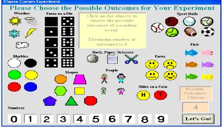
Figure 1 Designing an Experiment in Probability Explorer ...23
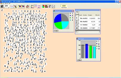
Figure 2 The Home Screen in Probability Explorer Showing the Results of Simulations ...24
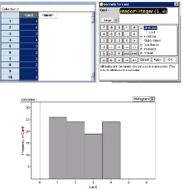
Figure 3 Simulating Random Integers in Fathom...26
Figure 4 Collecting Measures and Generating Dot Plots in Fathom ...27
Figure 5 Generating Random Numbers in Excel ...28
Figure 6 “Count If” Command in Excel ...29
Figure 7 Generating Random Integers in a Graphing Calculator ...30
Figure 8 The Informal Inference Task Teachers Solved ...37
Figure 9 An Organization of the Problem-Solving Pattern and Related Questions ...39
Figure 10 Two Data Tables of the Simulated Results of Two Samples in Probability Explorer ...49
Figure 11 Two Tables of the Simulated Results of Two Samples (Size 387) in Excel ....50
Figure 12 A Dot Plot in Fathom of the Number of Hats for 100 Simulated Samples (Size 93) ...51
Figure 13 A Spreadsheet in Excel Showcasing Formal Procedures ...52
Figure 14 Number of Repeated Samples Teachers Took Using Probability Explorer ....61
Figure 15 Number of Repeated Samples Teachers Took Using Excel ...69
CHAPTER 1 INTRODUCTION
In the current age of access to volumes of data, it is increasingly important that we are able to analyze and make inferences appropriately. Every day we read about studies citing statistics, or making claims about how one program or prescription is better than another. Policies that affect our entire society are often based on the results of experiments,
observational studies, and surveys. Because of this, it is vital that all citizens have a basic level of statistical literacy that allows them to ask insightful questions about how data was collected and what techniques were used for analysis instead of blindly accepting another person’s conclusions as fact. By teaching students how to interpret and evaluate various types of data, teachers play an essential role in educating students to make them better citizens in society (Garfield & Ben-Zvi, 2008).
With the introduction of the Common Core Standards (CCSSM, National Governors Association Center for Best Practices, Council of Chief State School Officers, 2010),
mathematics educators will be expected to teach big statistical ideas beginning in sixth grade and continuing throughout high school. For example, some of the topics students will be expected to learn are: sampling variability, describing distributions, using random sampling to make inferences, comparing two populations, and making inferences based on
that are based on data” (NCTM, 2000, p. 248). Specifically, high school students were expected to “use simulations to explore the variability of sample statistics from a known population and to construct sampling distributions,” and “understand how sample statistics reflect the values of population parameters and use sampling distributions as the basis for informal inference” (NCTM, 2000, p. 324). Based on these popular standards, statistical inference is a major topic that requires our attention.
Statistical inference has generally been regarded a difficult topic for students to understand – resulting in the need for learning about informal inferential reasoning first (Zieffler, Garfield, delMas & Reading, 2008; Makar & Rubin, 2009). Zieffler et al. (2008) and Makar & Rubin (2009) have suggested frameworks to help support future research on informal inferential reasoning, and offered examples of activities that help students learn about informal inference. These frameworks are designed to be broad in nature, allowing for activities at the elementary school level, or as complex as high school tasks. According to Makar and Rubin (2009), informal inferential reasoning in statistics is “the process of making probabilistic generalizations from (evidence with) data that extend beyond the data collected” (p. 83). Students can engage in an informal inference task by designing an experiment, collecting data, and making inferences using their data as supportive evidence.
inference tasks because students are involved in collecting and analyzing the data, and then they must either interpret salient features of the data or draw inferences. The teacher’s role is to design or choose open-ended tasks that will be appropriate for his/her students.
Additionally, the teacher should ask focused questions to keep the students engaged in task and attentive to the data being collected. While this sounds simple enough, teachers often struggle to ask questions that will deepen students’ understanding of the statistical topic they are learning (Lee & Mojica, 2008; Leavy, 2010).
In addition to choosing appropriate tasks and asking deeper questions, teachers also need to have the necessary content knowledge of the statistical topics embedded in informal inference. First, teachers need to know about samples, and that randomly selected samples accurately reflect characteristics of the population (Konold & Higgins, 2003). Second,
teachers need to be aware of the relationship between expectation and variation, and how that relationship is affected by sample size (Watson, Callingham, & Kelly, 2007). Finally,
teachers need to know that different samples yield different statistics, and that appropriate variation is difficult to intuitively predict (Watson & Kelly, 2004).
design experiments and collect data through simulation. After gaining experience with hands-on simulatihands-ons, such as flipping a coin or rolling a dice, it is more efficient to use computer simulations (Drier, 2001; Rossman & Chance, 1999; Ben-Zvi, 2000). The use of simulations is also suggested by NCTM (2000) and CCSSM (2010).
informal inference task. By collecting simulated data for a real-world context, students can begin to observe the differences that occur between samples, and they will be able to
determine which statistics are typical, and which would be considered unusual. Teachers can help guide this process by modeling problems, and by direct questioning or small group discussions. This will help lay the conceptual foundations students will need when they eventually encounter formal statistical inference.
Statement of the Problem
CHAPTER 2 LITERATURE REVIEW
Informal statistical inference is a relatively new research topic that encompasses many statistical topics and has varying levels of complexity. The purpose of this review of the literature is to consider the research that has already been done and determine a cohesive way of viewing the major facets of informal inference. This literature review distinguishes formal and informal statistical inference, identifies common statistical ideas within informal inference problems, describes the role of technology in solving these problems, and considers the part that teachers play in teaching these topics.
Informal Statistical Inference
Formal statistical inference is notoriously difficult to teach which is one reason why informal statistical inference is now being taught at the 6-12 grade levels. According to Wild, Pfannkuch, Regan, and Horton (2011), the term ‘statistical inference’ refers “to the territory that is addressed by confidence intervals, critical values, p-values, and posterior
knowledge. Throughout the investigation of these tasks, students can build an understanding of samples, statistical measurements, variability, distributions, etc. Formal statistical
inference requires not only an understanding of these big ideas, but also how to use what is observed to make conclusions. In order to develop an intuitive understanding of these processes, informal statistical inference plays a key role in building the conceptual groundwork that students will need.
Frameworks for Informal Statistical Inference
Several theoretical frameworks exist that help define and outline informal statistical inference. The Informal Inferential Reasoning (IIR) Framework, created by Zieffler et al. (2008), highlights three main ideas: making judgments or predictions based on data without using formal methods, using prior statistical knowledge, and making final claims about the population using data from samples (p. 45). Makar and Rubin (2009) also state the
importance of making generalizations about the population with supporting evidence from the data, but they add the importance of using probabilistic language to indicate a level of certainty about conclusions. Vallecillos and Moreno (2002) determined four major
constructs needed to engage in statistical inference: the relationship between populations and samples, the inferential process, sample sizes, and sampling types and biases. While these topics were not mentioned as part of an informal framework, since they are for “elementary” inferential statistics, they would be useful topics to consider in informal inferential reasoning.
Good tasks typically follow the PCAI model (Graham, 1987; Friel, O’Connor, & Manner, 2006), which highlights portions of a statistical investigation. Students should first pose the question(s), engage in collecting data, analyzing data, and then interpreting the results. Students will typically be given a contextual problem for which they have to formulate questions that can be answered by data. After they have formulated their questions, they must collect data, which could be from a randomized process such as simulations. Then, students would analyze the distribution of data using appropriate methods, and finally, they would draw conclusions or make inferences in the context of the problem by using the data as supporting evidence. This type of process supports informal inferential reasoning because the task is generally open-ended, and students would utilize the methods they know in order to justify their conclusions.
Samples
One of the main concepts needed to engage in informal inference is the idea of a sample. For the vast majority of problems we encounter in life, it is impractical to know every single unit of a population of interest. Because of this, we take one or more samples to learn information about the population without expending too much time or money. By taking samples from a population, we are collecting data that gives us information about the population. If samples are collected properly, then conclusions or predictions can be made about the population by using the sample as supporting evidence.
do not want to generalize from samples because “(a) you can only know about the cases you observe [and] (b) to characterize a group, you must test every member of that group” (p. 196). Students appear to recognize that units in the population differ from one another, but they seem to have trouble accepting that one can make generalizations based upon the observed units if they are collected properly. For elementary school students who did accept making generalizations from a sample, they often favored biased sampling methods. For example, Konold and Higgins (2003) describe how students preferred self-selected samples, or techniques that emphasized “fairness” (p. 197). The reasoning behind this was to prevent feelings from being hurt, or to ensure that the individuals chosen would represent the population.
As students get older and become more experienced with collecting random samples, they begin to encounter other statistical ideas that should influence their conclusions. Several factors about the sample(s) need to be taken into consideration in order to make appropriate conclusions. These factors include: sample size, sampling variation, sampling distributions, and how the samples were collected. The following paragraphs will discuss these ideas along with common misconceptions associated with each.
Sample Size
coin flips, most people would expect two flips to be heads, even though such a small number of flips could produce very unbalanced results. A variation of this belief is the notion that subsections of a long sequence of events will also accurately reflect the true proportions of the population, even though long strings of the same event often occur. If students believe that small samples are just as likely to represent the population accurately as large samples, then they may not think it is necessary to collect large amounts of data in order to make their inferences.
The second belief that people tend to have is the “empirical law of large numbers,” which is the intuition “that a large sample is better than a small sample for estimating a population parameter” (Sedlmeier & Gigerenzer, 1997, p. 35). For instance, many people would predict that a random sample of 100 adult males would give an average height closer to the true population mean than the average height of a random sample of 10 adult males. This belief would indicate that students may have an intuitive understanding of an
appropriate way to collect data and draw conclusions, but various studies have suggested that students do not always apply the “empirical law of large numbers” even when it would be appropriate to take sample size into account.
generally utilized one of those types of tasks, they developed different conclusions. When participants answer frequency distribution tasks, they have to consider the results of one sample. The “empirical law of large numbers” tends to work for these tasks because participants only need to recognize that a larger sample is more likely to produce a statistic closer to the population parameter. In contrast, a sampling distribution task requires participants to consider a distribution of sample statistics from samples of a fixed size. According to Sedlmeier and Gigerenzer (1997) “the empirical law of large numbers by itself is not sufficient to explain how sample size affects the variance of sampling distribution” (p. 44). In order to accurately answer sampling distribution questions, participants must consider how multiple sample statistics will be spread out, and how that spread will differ based on the fixed sample size that is taken.
The role of sample size is a topic that is easy to understand in some respects, while difficult to understand in others. Many students understand that a larger sample size is more likely to give statistics closer to the population parameter than a smaller sample size.
Sampling Variation
One major type of sampling variation is variability within a sample. There are
different ways to measure the variability within a sample, such as the range, the interquartile range, or the standard deviation. Of these three measurements, standard deviation is typically the most difficult one for students to grasp. According to Garfield and Ben-Zvi (2008), understanding variability and center is important because “when comparing groups or making inferences, we need to look at center and spread together: the signal, and the noise around the signal” (p. 204). In order to build a student’s conception of variability, they suggest starting with informal activities, like noticing that individual values vary, and working up to formal numerical measures of variability. Students should also recognize that variability can be due to both measurement error and an indication of the diversity of the subjects being measured. Garfield and Ben-Zvi (2008) describe a task that would allow students to discover the types of variability through repeated measures of head circumference and the measurements of different students’ heads (p. 210). This type of lesson would allow students to reason about variability informally first, so they will be better equipped to learn about specific measurements of variability, such as standard deviation.
samples can differ from one another, and use that knowledge to make sound judgments and express degrees of uncertainty. According to Wild, Pfannkuch, Regan, and Horton (2011), “any conceptual approach to statistical inference must flow from some essential
understandings about the nature and behavior of sampling variation” (p. 253). Thus, it is imperative that students have a solid understanding of variation between samples, so they can consider which statistical measurement values are likely and unlikely to occur.
In the past it has been difficult to gauge students’ understanding of variation between samples because most test items asked for the theoretical value instead of a range of values. To remedy this lack of research, Watson and Kelly (2004) created a questionnaire that asked students to write a list of six sets that would give appropriate estimates for the number of times a spinner would land on the shaded part after 50 spins. If a student wrote the same number six times, then this showed a lack of appreciation for variation between samples. In contrast, if a student wrote six different numbers that encompassed more extreme values than one would expect, then this would indicate a lack of awareness about appropriate variation. Other questions on this questionnaire gave visual depictions of 27 sets of 50 spins for the same spinner. Two of these dot plots were made up; one distribution was perfectly
test items. Students seemed to have an appreciation for “randomness” in the sense that a perfectly symmetrical distribution is unlikely to occur for such a small number of sets, but the belief that “anything can happen” is still ingrained in many students, even after
instruction. This acceptance of unreasonable variation can make it difficult for students in informal inference tasks, because they might reach conclusions that allow for more variation than their data suggests.
Sample size plays a key role in variation between samples that is not very intuitive. While students may recognize that a larger sample size yields statistics closer to the true parameter, they have difficulty connecting this to a lower variance between sample statistics. According to Sedlmeier and Gigerenzer (1997), students perform better with frequency distribution problems because they are involved in real-life issues, “whereas the rule that the variability of a sampling distribution decreases with increasing sample size seems to have only few applications in ordinary life” (p. 46). In practice, we often make inferences on one sample, but it is necessary to consider how the statistics of different sample sizes vary in order to validate our conclusions.
Sampling Variation with Respect to Expectation
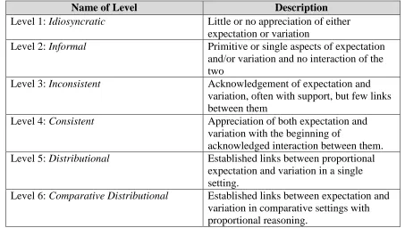
understanding of expectation and variation, and the relationship between the two. The coding scheme Watson, Callingham, and Kelly (2007) developed is shown below, with a brief description of each level (p. 93).
Table 1: A Table Describing Watson et al.’s (2007) Coding Scheme for Variation and Expectation
Name of Level Description
Level 1: Idiosyncratic Little or no appreciation of either expectation or variation
Level 2: Informal Primitive or single aspects of expectation and/or variation and no interaction of the two
Level 3: Inconsistent Acknowledgement of expectation and variation, often with support, but few links between them
Level 4: Consistent Appreciation of both expectation and variation with the beginning of
acknowledged interaction between them. Level 5: Distributional Established links between proportional
expectation and variation in a single setting.
Level 6: Comparative Distributional Established links between expectation and variation in comparative settings with proportional reasoning.
considering expectation or variation in the context of the problem, but not realizing that both were present. The Inconsistent level was reserved for students who answered the question with inconsistent responses. An example given of this was the response “Anything can happen” in conjunction with phrases like “50-50” (p. 99). They also tended to focus on single features of expectation or variation, like describing one thing as being more than something else, instead of providing a range of values. In contrast, students at the Consistent level “were likely to recognize the need for consistency in suggesting ranges in relation to data values and, when specifically asked for explanations of words associated with variation, generally provided satisfactory responses for all terms” (p. 101). The Distributional level was reserved for students who could describe the relationship between expectation and variation in a single data set without much prompting. Students often mentioned the shape, and how values vary around an expected center. The highest achievable level, Comparative Distributional, met the requirements of the previous level and students were able to compare the expectations and variations for two different samples. These levels are intended to be hierarchical, and Watson et al. (2007) suggest using these codes to determine where students are developmentally so that appropriate tasks can be used to help them progress to the next level.
Sampling Distributions
successfully teach (Aguinis & Branstetter, 2007; Gourgey, 2000; Wybraniec & Wilmoth, 1999; Zerbolio, 1989). There are numerous reasons why the topic of theoretical sampling distributions is so difficult to understand. Before learning about theoretical sampling distributions, students typically first learn about parent distributions and a distribution of a sample. In order to truly understand sampling distributions, students need to compare them to the parent distribution, and they need to distinguish between an empirical sampling distribution and a distribution of a sample. The language used for the latter two is very similar, which probably does not help students understand that an empirical sampling distribution focuses on the statistics of multiple samples instead of just one sample.
Theoretical sampling distributions are often difficult to teach because they combine several different statistical ideas that are all important in understanding its underlying structure. Not only do students need to know about the statistic of a sample, how the sample size affects that statistic, how statistics can vary, and how values can be distributed, they also need to be able to put all of that together, and compare it to both the parent population and theoretical sampling distributions for other fixed sample sizes. If students have not mastered all of the aforementioned ideas, then they will be missing a necessary piece of the puzzle required to understand this complex topic.
first finding in a study about undergraduates answering questions about a theoretical hospital. Only 20% of the 95 Stanford undergraduates correctly answered that a smaller sample would more often have more than 60% boys born on a given day. According to Watson and Moritz (2000), the reason the students had trouble with this question is because the questions are complex and “involve comparison of the tails of the sampling distribution of large and small samples” (p. 46). The hospital problem was also used in a study about students in grades 5 through 11. Fischbein and Schnarch (1997) argue that students focused more on the ratio for the hospitals (and thus believed that the number of days for the small and large hospital would be equal) instead of considering the relevancy of sample size.
The second major finding about sampling distribution research is that students often have difficulty determining whether a question is asking about a sampling distribution or a frequency distribution. Three pieces of evidence support this theory. According to
The topic of sampling distributions is difficult to teach, and it takes time to teach it well. Often text books can illustrate basic concepts adequately, but many text books briefly describe a theoretical sampling distribution, and then discuss how they can be used without going into much depth. Many teachers recognize the deficiencies in the text-book based approach, so they often begin by doing a hands-on activity with an empirical sampling distribution in which students each take a sample and then plot their sample statistic on a dot plot. Wybraniec and Wilmoth (1999) utilized a hands-on activity with sampling blocks, and stated that students’ “comments during class discussion and interpretations on the exams indicated that they understood the reason these procedures are necessary for making inferences” (p. 80). While this approach helps to introduce the idea of how a sampling distribution is constructed and how one can make inferences based on the sampling
distribution, it does not necessarily help students make broad generalizations about the effect of sample size on sampling distributions. To create multiple empirical sampling distributions by hand would require more time than most instructors are willing to sacrifice, so many choose to use technology for further explorations.
Sample Collection
their inferences (p. 302). Without recognizing the need for randomization when designing an experiment, students will not have a fundamental grasp on when it is appropriate for
inferences to be made. Giving students the opportunity to collect data is a crucial part of the informal inference process because it serves as the foundation upon which the inferences are formed.
Simulations
One way to collect samples is through simulations. A simulation is letting one event represent something else in order to easily repeat the event to construct a data set; for example, if the odds of having a baby girl is 50%, then you could let a coin flip of “heads” represent having a girl, assuming a fair coin. The purpose of simulations is generally to make some predictions of what is reasonable or unreasonable based upon the results of several simulations. Simulations are random in the sense that the observer cannot predict with accuracy what sequence of events will occur. Batanero, Green, and Serrano (1998) described a study in which children were posed with two sequences (one random, and one non-random) of 150 coin flips; when asked which sequence was more likely to represent 150 coin flips, “most of the children chose the non-random sequence, and the perception of randomness did not improve with age” (p. 120). Some of the incorrect reasons that children gave were that the strings of heads or tails were too long, or the results were not exactly fifty percent for each. Children tend to have expectations about what should happen, and they may not accept the randomness of events.
observing physical simulations of an event. According to Rossman and Chance (1999), it is best for students to use “physical simulations to become comfortable with the idea of repeated samples,” (p. 299) before beginning the use of technology to perform simulations. Hands-on simulations can occur in a variety of ways, such as coin flips, tossing dice, sampling marbles, etc. Discussions about sampling with and without replacement, and the unpredictable sequences in the results can extend naturally from these types of simulations. By allowing students to experience simulations in a hands-on way first, they will be better equipped to understand what is being simulated in a computer environment.
Many different technologies exist that allow users to easily run simulations. In some cases, the results of the simulations are represented in tables or charts, while in other
technologies the results are depicted visually. According to Ben-Zvi (2000), “technological tools support enhanced accessibility of many statistical conceptions by permitting the
transformation of purely symbolic presentations into spatial-geometric ones, which are easier to grasp and build cognitive models on” (p. 142). Thus, while many students may not
understand formal statistical notation, technology can allow them to see the illustration of a statistical topic. Some of these technologies, like applets, may have predetermined features that are designed to demonstrate specific statistical topics, such as sampling distributions or confidence intervals. These technologies may also focus on specific facets of the larger topic in order to draw the user’s attention to a specific idea. Rossman and Chance (1999) state that “technology can also free students from computational drudgery, allowing them to
sample size or confidence level” (p. 299). By quickly allowing users to make comparisons between large and small samples, students can make generalizations more easily. Other technologies allow the user to design an experiment and run a particular number of
simulations. Some of these technologies, like Probability Explorer (v. 2.01, Stohl, 2002) and Fathom (v.2.11, KeyPress Technologies), may be more educational in nature, while others, like Excel and the graphing calculator, may be designed for other practical uses.
Probability Explorer
Figure 2: The Home Screen in Probability Explorer Showing the Results of Simulations
children to use graphs both as objects of display after a simulation is complete and as objects of analysis during a simulation” (p. 23). One of the drawbacks to this program is that while it can help students build the conception of a simulation, it does not perform simulations
quickly or allow an easy storage of the results of several simulations for students who want to analyze the data further. Although there are limitations to what it is capable of doing,
Probability Explorer is an excellent tool to help build informal inferential reasoning because it gives users the opportunity to collect data in a meaningful way, and then make judgments based on that data.
Fathom
Fathom is another interactive computer program that allows users to build statistical knowledge. While Probability Explorer is directed towards a younger audience, Fathom offers more formal statistical features that would be useful in a high school or introductory college statistics class. According to Meletiou-Mavrotheris (2003), “The designers of Fathom have drawn on constructivist theories of learning as well as several years of academic
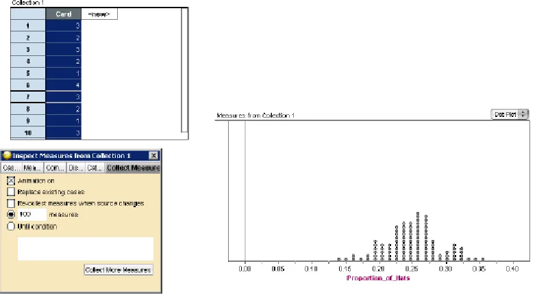
Figure 4: Collecting Measures and Generating Dot Plots in Fathom
According to Meletiou-Mavrotheris (2003), the “Collect Measures” feature “can collect the statistic from repeated samples taken from the original population” (p. 273). This feature is useful because multiple samples can be run at the same time, and the statistics of interest can be collected and stored in an efficient manner. Based on these collected statistics, users can generate graphics like dot plots. This feature gives students the opportunity to see an empirical sampling distribution based on their data. Although Fathom visually
Microsoft Excel
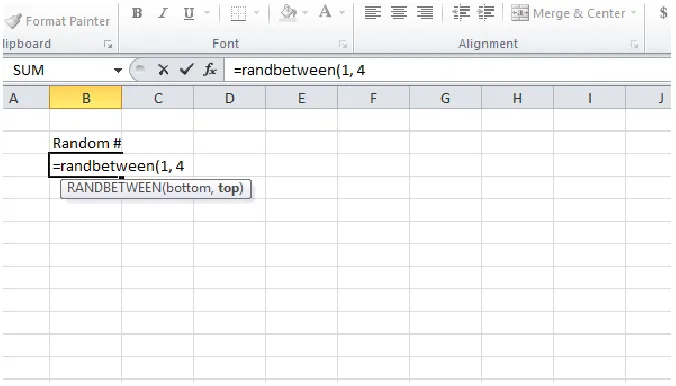
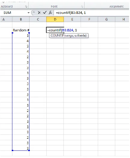
Some technologies that run simulations were primarily designed for other uses as well. For example, Microsoft Excel (2007) is a computer program designed to organize data in a spreadsheet, but it can also compute simple statistical measures and run simulations. Users can randomly generate numbers by using the “randbetween( )” feature, and can tally the value of their choice by using the “countif( )” command. Screenshots of these commands in Excel are shown below.
Figure 6: “Count If” Command in Excel
update the diagram chart because “when the sample means change (every time function key F9 to recalculate is depressed), the frequency counts will automatically be updated, which in turn will update the histogram” (p. 37). While it is conceivable to simulate multiple samples at the same time in Excel, it is not intuitive or easy to learn for beginners. In spite of its complicated formulas, Excel has the advantage of being ubiquitous, whereas Fathom and Probability Explorer are not as readily available for teacher use.
Graphing Calculator
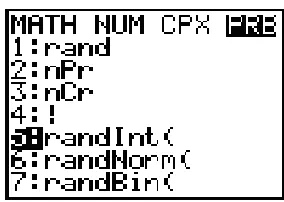
Another tool that is widespread in most mathematics classrooms is the graphing calculator, which also has the ability to run simulations. Users can run simulations on the graphing calculator by using the “randINT( )” function, and the values that are given can be stored in a list. Using the “randINT( )” function on the graphing calculator is shown in the screenshot below.
Figure 7: Generating Random Integers in a Graphing Calculator
mean, and repeat the process in order to have a collection of sample means. Although it is possible to build a collection of statistics, this would be very time-consuming, and the graphics offered on the calculator do not include dot plots, so the empirical sampling distribution would have to be viewed as a histogram. Additionally, if all students in a classroom are running simulations for the same problem, the teacher would need to tell the students to choose different seed values so the simulations will generate different results. It is not impossible to create an activity with the graphing calculator to build empirical sampling distributions, but aside from its ubiquity, it does not offer many advantages over other technologies.
The Teacher’s Role
Additionally, while teachers may know how to calculate common statistics like the mean or standard deviation, they do not necessarily recognize these as tools to be used in data analysis. According to Makar and Rubin (2009), “it is vital that the focus in using statistical tools is embedded in the reason that we do statistics – to understand underlying phenomena” (p. 84). In order to teach informal inferential reasoning successfully, teachers need to realize that statistical tools can help students make inferences, but they should not be the
culminating result.
Once teachers have the required content knowledge, they need to be able to transform that to pedagogical content knowledge. Teachers need to be able to choose open-ended tasks that are appropriate for their students, and they need to know appropriate questions to ask that will keep students focused on making inferences by supporting them with data. Leavy (2010), described a study of 26 Irish pre-service teachers who worked in groups of five or six to design a lesson study that focused on a statistical activity which would incorporate major components of statistical inference. From this study, two observations were made: teachers had difficulty using effective questioning to build informal inference, and teachers did not always know how to handle unanticipated responses from children. Because of this, Leavy (2010) suggests that “there was a failure to focus children on analysis of the data, the identification of patterns, and the generation of assertions arising from those patterns” (p. 57). In terms of questioning, the teachers did not recognize the importance of using data as evidence for the inferences being made, so they did not ask students to justify their
one result would be better than another before considering the data, caught teachers off-guard and redirected the focus of the lesson away from the data. This suggests some challenges that teachers face when giving open-ended tasks to their students. Teachers must have good questions in mind to redirect students’ attention to the problem, and they need to be prepared for all types of responses from students.
In order to effectively teach some of the higher level informal inference tasks, teachers also need to have knowledge about the technologies they are planning on using in their classrooms. According to NCTM (2007), “if teachers are to learn how to create a positive environment that promotes collaborative problem solving, incorporates technology in a meaningful way, invites intellectual exploration, and supports student thinking, they themselves must experience learning in such an environment” (p. 119). Many different technologies exist that can be used for different types of tasks, with some illuminating concepts better than others. Teachers have to make a decision about which technology to use based on what is available, what will help students learn the topic best, and what students would need to learn about the technology itself.
Research Questions
unreasonable values, sample size, and using data to justify conclusions. The author chose the following research questions to focus on:
1. How do teachers use different technology tools to conduct simulations and make informal inferences?
CHAPTER 3 METHODOLOGY
A multiple case study methodology was used to analyze this data. According to Baxter and Jack (2008), “a multiple case study enables the researcher to explore differences within and between cases” (p. 548). This observational study utilized written documents by teachers as they used a technology of their choice to solve an informal inference problem. The cases were defined by three of the technologies teachers could use in a simulation task, with each case having multiple teachers’ responses. The purpose of choosing technology type to determine the cases was to explore the similarities and differences between how teachers formed their conclusions and how their technology choice may have influenced those conclusions. This chapter seeks to address the context of the study, the data used, and the analysis techniques employed to examine the cases.
Larger Study
The data for this study is a part of a larger study that considered how teachers utilized dynamic statistical software to solve three exploratory data analysis tasks. According to Lee, Kersaint, Harper, Driskell, and Leatham (2012), the “research group examined teachers’ use of dynamic statistical technology environments with teachers enrolled in courses from eight different institutions in the United States in which faculty were using the same curriculum materials” (p. 291). The curriculum materials came from Preparing to Teach Mathematics with Technology: An Integrated Approach to Data Analysis and Probability (Lee,
Instructors at each institution were able to choose whether their teachers participated in each task.
Context for the Study
Figure 8: The Informal Inference Task Teachers Solved
although only four teachers used Fathom, I chose to include those responses because it was clear how the teachers used that technology tool to solve the problem. After excluding the graphing calculator responses, this left a total of 57 responses, grouped among three different cases.
Analysis Techniques
Before I read any teachers’ responses, I attempted to solve the task using the different types of technologies to get a sense for how one might go about solving such a task
informally. Then I tried to pinpoint the technological and statistical skills that were needed to solve the task. To gain an awareness of how teachers solved the task, I read a few of the responses to see how they were structured.
Responses were separated into the three cases. I read each response and made general notes about the approaches used. Based on the nature of the task and on the review of
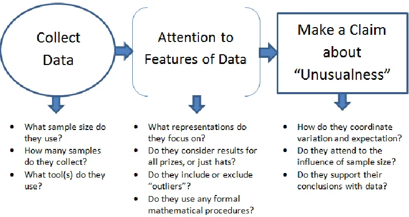
answered about each response. The bulleted questions below the diagram offer a preview for what my coding schemes will focus upon.
Figure 9: An Organization of the Problem-Solving Pattern and Related Questions
Coding Initial Expectations for the Proportion
The second portion of part (a) in the informal inference task (Figure 8) requires teachers to determine reasonable expectations for the proportion of customers who will receive hats over the weekend. This prompt does not give an associated sample size, so teachers have to determine whether to provide a range of values, and if they do, what sample size to base that range on. In order to code the initial expectations for the proportion, a
Table 2: Coding Scheme for Initial Expectations for the Proportion
Inconsistent – 0 Pre-Consistent – 1 Consistent – 2 Distributional – 3 • Not recognizing
appropriate variation of expectation • Too much variation: Belief that “anything can happen”
• No variation: Point estimate
• Listing single value based on one sample (of any size) • Recognizing some variation: “about 25%” but without an associated range
• Appreciation of variation around a reasonable center (but too much or too little)
• A reasonable range, but no indication of the sample size or data used to construct
• Appropriate range around 25% based on sample(s) OR
• Based on thoughts of how the range would differ based on different sample sizes
Some of the levels described by Watson et al. (2007) were not included in this coding scheme because they were either too simplistic for this group of teachers, or they were too complex for the initial question. Additionally, the levels that were utilized were modified to match the details of this task. Each of these levels is described below.
Teachers operating at the Inconsistent level (0) either had an expectation of far too much variation for the proportion, or did not appreciate any variation and believed that the expected proportion would be exactly 0.25. Teachers functioning at the Pre-Consistent level (1) either simulated one sample of any size, and listed a single value based on that sample, or they stated that the expected proportion would be “about 25%.” This level was not in the original framework, but it was added out of necessity to bridge the gap between the
level if the range they provided was reasonable, but there was no indication of the sample size or data used to construct it. This would be coded Consistent instead of Distributional because the range provided may not be appropriate depending on the sample size for the weekend. The Distributional level (3) was the highest possible code for the initial expectations. Teachers who were coded at this level either provided an appropriate range based on sample(s) of a specified size, or they made statements comparing the ranges for hypothetical sample sizes. For example, if a teacher said that a larger sample size would produce a smaller range of proportions around 0.25, then that response would be coded as Distributional.
Coding Variation with Respect to Sample Size
Table 3: Coding Scheme for Variation with Respect to Sample Size
Inconsistent – 0
Distributional – 1 Pre-Comparative Distributional – 2
Comparative Distributional – 3
Explanatory Comparative – 4 • No appreciation for appropriate variation • “Anything can happen” OR • Exactly 25% for each sample size
• Same proportion ranges for Friday and Saturday (no appreciation for sample size) • Weak
appreciation for two aspects, but not for the third (aspects:
variation, expectation, sample size)
• Ranges based on data but given too much extra “wiggle room” • Inappropriate variation with respect to sample size, but based on empirical
evidence • Fairly reasonable range(s), but no indication of the data used to construct it
• Reasonable ranges with appropriate variation
provided for the different sample sizes
• Meets the requirements of Level 3 AND • Explicitly states that a larger sample size would produce values more likely to be closer to the expectation (less variation)
Teachers operating at the Inconsistent level (0) were very similar to those for the initial expectation in the sense that there was no appreciation for appropriate variation. For this coding scheme, the Pre-Consistent and Consistent levels were left out because teachers either operated at an Inconsistent level, or they operated at a Distributional level that did not make appropriate comparisons for different sample sizes. In this instance, teachers
sample size. Because they missed this crucial piece of the problem, they would be coded at the Distributional level.
The Pre-Comparative Distributional level (2) was added to transition between the Distributional and Comparative Distributional levels. Teachers were coded as
Pre-Comparative Distributional when they provided ranges that were based on data, but they widened the range to include proportions that had a very low probability of occurring. These ranges tended to be narrower proportionally for the higher sample size, but they still
encompassed an inappropriate amount of variation. A teacher could also be coded at this level if the ranges were based entirely on empirical evidence, but the variation for the higher sample size was larger. While the ranges were based on data, the teacher could have
recognized that the extreme values rarely came up for the larger sample size, so s/he is showing a lack of observation about typical variations. The final type of response that was coded as Pre-Comparative Distributional occurred when a teacher gave a range or ranges that were fairly reasonable, but did not indicate where the numbers came from or how they were found.
operating at this level have an understanding of expected proportions, variation around those proportions, and how that variation is different for different sample sizes. Since this task did not specifically ask teachers to explain the differences in variation, the Comparative
Distributional level for this particular task does not require an explanation about the
variation. However, since so many teachers did elaborate about variation in their responses, a fourth level was created named Explanatory Comparative Distributional level (4). Teachers operating at this level meet the requirements of the previous level, and explain that larger sample sizes tend to have less variation of sample proportions while smaller sample sizes tend to have more variation of sample proportions.
Coding Repeated Sampling
51 or more samples taken. These categories do not have the same numeric width because I interpreted a larger difference in how students approached the problem for lower numbers vs. higher numbers. For example, I think a teacher who took two samples compared to a teacher who took five samples should be in different categories because the teacher who took more samples is showing an awareness that more samples will give more information. However, I do not think that teachers who did 100 repeated samples vs. 103 repeated samples should be placed in different categories because a difference of three in such a large number of samples is negligible. Based on this premise, I chose to make the ranges for the beginning intervals smaller, while they gradually became larger to encompass more types of responses.
An issue that came up while coding each response was the use of language eight teachers utilized. Instead of specifying the exact number of samples they took for each day, they used words like “several,” “many,” “numerous,” etc. In order to analyze these
responses with the rest of them, I placed them in the 5 to 9 category. It is my supposition that when we use words like several or many, we mean approximately more than two, and likely a relatively large amount. But without specification, it is reasonable to assign these terms to the category of less than 10.
After coding the responses to be in a numeric category, it was evident that some of the categories had many more responses than others, and it was difficult to notice trends when the numbers for the categories were so unbalanced. To remedy this, I decided to create three general categories for types of samplers: low, medium, and high. Teachers who took 0 to 4 samples were considered “low samplers,” 5 to 20 samples taken were “medium
samplers,” and 21 or more samples taken were “high samplers.” Again, the numeric widths are not the same for the reasons previously mentioned. By narrowing it down to three
categories, the numbers became more comparable and trends were easier to notice. I am also more comfortable doing this because I feel confident that the teachers who wrote about taking “several” or “multiple” samples should be included in the “medium samplers” category.
Formation of Conclusions
them rather than asking those data to yield responses required by the issues or hypothesis that guided their collection.” (p. 425). Thus, my approach to this study included both propositions for analysis, as well as a pseudo-grounded theory approach. I decided upon seven main categories for forming conclusions, with an eighth category for conclusions that were unclear. The categories are listed and briefly described in the table below.
Table 4: Types of Conclusions Formed with Descriptions
Type of Conclusion Brief Description
Unsupported by Data Conclusions were not supported by data
Extremes for Any Outcome Ranges built using extreme numbers for any outcome Extremes for Specified
Outcome
Ranges built using extreme numbers for specified outcome
Excluding Extreme Values Ranges built excluding observed extreme values Formal Procedure Formal statistical procedure used to build ranges Informal Procedure Informal procedure used to build ranges
Multiple Strategies More than one strategy used to build ranges Unclear Strategy Strategy used was not clear
s/he made no distinction between alarming percentages for Friday and Saturday. While the assumption may not be invalid, it is not supported by evidence because the teacher does not explain how those numbers were found, and screenshots do not support the statement.
Figure 10: Two Data Tables of the Simulated Results of Two Samples in Probability Explorer
At the beginning of the teacher’s response, s/he stated that the number 3 represented the hat. However, in the three samples that were simulated, the hat came up 21, 23, and 24 times. Interestingly, these numbers were not used to build the range. Based on the screenshots, it is my supposition that the teacher used the lowest (18) and the highest (26) values for any prize to build the range. This type of response would be coded as “Extremes for Any Outcome.”
Figure 11: Two Tables of the Simulated Results of Two Samples (size 387) in Excel
The teacher then states that “On Saturday, up to approximately 118 hats or as few as 85 of hats can be given away.” While 118 is the high extreme for any of the prizes, 85 is not the low extreme of all of the prizes. Based on the teacher’s given range and the screenshot, it appears that s/he is only looking at the extreme values of hats to build the range. Therefore, this response would be coded as “Extremes for Specified Outcome” because the teacher is only considering the data for the particular prize of hats.
often, decided not to include them to build the ranges. Other teachers used screenshots to help support their conclusions, and made it easier to determine that they had in fact excluded the most extreme values. For example, one teacher included the following in the response:
Figure 12: A Dot Plot in Fathom of the Number of Hats for 100 Simulated Samples (size 93)
The teacher then states that an acceptable range for Friday would be between 16 and 32 hats. Based on the screenshot, you can observe that one value is below 16 hats and one value is above 32 hats. Because of the range given in comparison to the screenshot, this response would be coded as “Excluding Extreme Values”
A few teachers did not fit into any of the previous categories, but they did write about their techniques for solving the problem. The following categories did not have many
responses, but to be true to the teachers’ descriptions I decided to include them. The first Friday
14 16 18 20 22 24 26 28 30 32 34 36
mean = 23.85 mean s = 19.6858 mean +s = 28.0142
median = 24
mean s = 15.5215
mean + s = 32.1785
category is “Formal Procedure.” Responses were coded “Formal Procedure” if teachers used formal statistical procedures to solve the problem. For example, one teacher performed Chi-Square tests in Microsoft Excel to determine whether individual values would be considered unusual. Another teacher was coded as “Formal Procedure” because s/he ran ten simulations and then found the mean and standard deviation to help determine a range of acceptable values. The screenshot used for that response is shown below.
Figure 13: A Spreadsheet in Excel Showcasing Formal Procedures
Responses were coded as “Informal Procedure” if the mathematical procedure or organization used was very simplistic and/or did not make sense. For example, one teacher ran two simulations each for Friday and Saturday, and then added the low values to
considering how far those percentages deviated from the expected value. A few responses were coded as “Multiple Strategies” because a teacher utilized a combination of the
strategies. For example, one teacher focused on the extreme values for hats on Friday, but excluded the most extreme values of hats for Saturday. Since two different strategies were employed for Friday and Saturday, this was coded as “Multiple Strategies.”
Other responses were not placed in any of the aforementioned categories because it was not clear what approach the teacher decided to take. These occurred for a few different reasons. First, some teachers did not actually state any ranges for Friday or Saturday, so none of the previous categories would make sense for those teachers. Second, some teachers determined reasonable ranges for Friday and Saturday, but they were vague in their descriptions and/or their screenshots did not match up with their ranges. Finally, some teachers indicated that they chose extreme values to build the ranges, but it was not obvious whether they were choosing an extreme number based only on hats, or an extreme number based on any prize. Because of this lack of clarity, responses that met the previous criteria were coded as “Unclear Strategy.”
Looking Across Cases
type of sampler a teacher was considered, it was easier to determine how the type of sampler was related to the types of conclusions. Additionally, the number of samples simulated also appeared to be related to the reasoning levels for part (b) of the task, so a cross-analysis of the two variables was done as well.
CHAPTER 4
RESULTS BY TECHNOLOGY CASE
The purpose of this chapter is to describe the teachers’ work on the task for each of the different cases of technology type. This chapter will be organized into three major sections examining responses for Probability Explorer, Excel, and Fathom. Each section will include a general description of the documents as well as the most popular justifications for that choice of technology. The sections will also indicate the levels for the initial
expectations as well as the final expectations for the proportion of hats for each technology case. Finally, trends in repeated sampling and the formation of conclusions will also be shown for each technology case. A fourth section will highlight the main similarities and differences between the technology cases.
Probability Explorer
Reasons for Choosing Probability Explorer
The first part of the task asked teachers to justify their choice in technology. While five teachers did not answer this part of the task, the rest of the Probability Explorer users did. The following table shows the most common reasons for using Probability Explorer, along with the percentages of teachers who specified each reason.
Table 5: Top Justifications for Choosing Probability Explorer
Justification Frequency Percentage (out of 31)
Dynamic Nature 16 52%
Ease of Use 14 45%
Available Representations 12 39%
Fun/Entertaining 6 19%
Speed 4 13%
the appropriate sample sizes. Twelve teachers stated that the available representations (data table, pie graph, bar graph) were another advantage in this technology choice because these features were automatically available. Finally, six teachers said that the program was fun and entertaining to use, while four teachers stated that the speed of the simulations was an
advantage. Most teachers who answered this part of the task gave multiple reasons, so they found several advantages to using Probability Explorer.
Initial Expectations for the Proportion of Hats
Table 6: The Reasoning Levels for Probability Explorer Users in Part (a)
Part (a) Reasoning Levels for Expectation of Proportion for
Probability Explorer Users
Level Frequency
Percent (out of 27)
Inconsistent – 0 1 3.70
Pre-Consistent – 1 5 18.52
Consistent – 2 6 22.22
Distributional – 3 15 55.56
Most of the teachers who answered this question were operating at the Distributional level, meaning that they gave an appropriate range around 25% grounded by specific sample sizes, or based on thoughts that described how ranges would differ based on sample size. Six teachers functioned at the Consistent level, implying that their ranges were somewhat
reasonable but gave too much or too little variation, or they may have been reasonable for specific sample sizes, but they did not include any data to support their conclusions. Teachers were most commonly coded as Consistent for the latter reason. Five teachers were working at the Pre-Consistent level, indicating that they either provided a single value for the
expectation based on a sample, or they stated that the proportion would be “around 0.25”, or “roughly ¼.” Four teachers at this level stated they believed the proportion would be
0.25), and it did not recognize appropriate variation for the expectation. The upper bound of 0.50 was far too high for the specified sample size of 500.
Reasoning About Variation with Respect to Sample Size
Part (b) of the task asked teachers to consider what number of hats given away would be considered unusual for two different sample sizes (93 and 387). Many teachers gave a range of values or proportions for each day that would be considered reasonable, and then stated that anything outside those ranges would be considered unusual. Each response was coded as Inconsistent (0), Distributional (1), Pre-Comparative Distributional (2),
Comparative Distributional (3), or Explanatory Comparative (4), as described in the previous chapter. Three teachers who used Probability Explorer did not answer this portion of the task, so they are excluded from the frequency table below.
Table 7: The Reasoning Levels for Probability Explorer Users in Part (b)
Part (b) Reasoning Levels for Comparing Variations of Two Different Sample Sizes for Probability Explorer Users
Level Frequency
Percent (out of 28)
Inconsistent – 0 3 10.71
Distributional – 1 4 14.29
Pre-Comparative – 2 6 21.43
Comparative – 3 5 17.86
Explanatory Comparative – 4
10 35.71
Fifteen teachers operated at the Comparative Distributional level or higher, which meant that they adequately answered this portion of the task by providing reasonable ranges with appropriate variation for each sample size; ten of these teachers explained the effect of sample size on the variation of sample proportions, which indicated they were functioning at the Explanatory Comparative level. Six teachers functioned at the Pre-Comparative
Distributional level, which indicates that although sample size influenced their ranges of acceptable values, they often added in extra “wiggle room” that encompassed an
inappropriate amount of variation, presumably to capture all possible values that might occur. Three teachers were coded as Distributional because although their conclusions supported a relationship between variation and sample size, they showed a lack of appreciation for expectation (0.25), and gave ranges where the expected proportion of 0.25 would be
considered unusual. A fourth teacher was coded as Distributional because s/he gave the same proportional ranges for both sample sizes, which showed a lack of awareness for how sample size affects the variation of proportions. Three teachers were coded at the lowest level, Inconsistent, because they did not have an awareness of appropriate variation by either providing a point estimate, or by picking arbitrary values that would contain inappropriate variation.
Engaging in Repeated Sampling