Abstract
RAO, SUNIL, MURALI. Tchebycheff Method-based Evolutionary Algorithm for
Multi-objective Optimization (Under the direction of Dr. Ranji Ranjithan)
In the operations research literature, the Tchebycheff method has been demonstrated to be a
useful approach for exploring the non-dominated solutions for multiobjective optimization
problems. While this method has been investigated with mathematical programming-based
solution approaches, its application with modern heuristic search procedures is lacking. As
heuristic search procedures continue to show promise as practical solution approaches for
realistic engineering problems typically with multiple design objectives, the need for their
applications in multiobjective optimization is becoming increasingly important. This
pa-per investigates a new evolutionary algorithm-based multiobjective optimization procedure
that builds upon the Tchebycheff method. By embedding a beneficial seeding approach,
the efficiency of the algorithm is expectedly enhanced. This Tchebycheff Method-based
Evolutionary Algorithm (TMEA) is tested and evaluated using a suite of 2-objective test
problems, representing a range of complexities in the decision space as well as in the
ob-jective space. The performance of TMEA with those of other multiobob-jective evolutionary
algorithms are compared using several performance metrics that are reported in the
litera-ture. For the problems considered in this paper, TMEA performs relatively well in
generat-ing non-dominated solutions that are close to the known Pareto set and are well distributed
TCHEBYCHEFF METHOD-BASED EVOLUTIONARY
ALGORITHM FOR MULTIOBJECTIVE OPTIMIZATION
BY
SUNIL M RAO
A THESIS SUBMITTED TO THE GRADUATE FACULTY OF NORTH CAROLINA STATE UNIVERSITY
IN PARTIAL FULFILLMENT OF THE REQUIREMENTS FOR THE DEGREE OF
MASTER OF SCIENCE
DEPARTMENT OF CIVIL, CONSTRUCTION AND ENVIRONMENTAL ENGINEERING
RALEIGH
JULY2003
APPROVED BY:
Biography
Sunil M. Rao was born on October 29, 1978. He was brought up in the coastal city of
Surat, Gujarat, India. He completed his schooling from St. Xaviers High School, Surat.
He joined Birla Vishwakarma Mahavidyalaya and obtained his Bachelors degree in Civil
Engineering in 2000. He joined the Masters program at North Carolina State University,
Raleigh in Civil Engineering in Fall 2001.
At NC State he undertook course-work in the areas of Environmental Systems
Anal-ysis and Computer Science and research under the direction of Dr. S. R. Ranjithan. His
research interests include application of optimization techniques to engineering problems
and software engineering and development.
Acknowledgments
I would like to thank my adviser and committee chairman Dr. S. R. Ranjithan for his
invaluable guidance and constant encouragement throughout the course of this work. I am
also grateful Dr. Downey Brill and Dr. John Baugh Jr. for being on my committee and
providing valuable comments on my thesis.
I would also like to thank my office mates, Emily , Siva and Parthee for their wonderful
friendship and also for sharing their ideas, opinions and experiences.
Lastly I would like to express my gratitude towards my parents, Dr. B. K. Murali and
Mrs. Saraswati Murali, for their love, support and for being a constant source of inspiration
throughout my education.
Table of Contents
List of Tables v
List of Figures vi
1 Introduction 1
2 The Tchebycheff Method 3
3 Tchebycheff Method-based EA 7
4 Evaluation of TMEA 10
5 Performance Assessment 13
6 Results 15
6.1 Unconstrained Test Problems . . . 15
6.2 Constrained Test Problems with Continuous Decision Variables . . . 15
6.3 Constrained Test Problem with Discrete Decision Variables . . . 22
7 Summary and Conclusions 26
List of References 28
A Computational Performance Evaluation of the TMEA 32
List of Tables
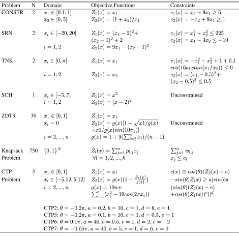
4.1 Test problems used in this study. The objective functions are denoted by
, , where denotes the number of objectives and the
number of decision variables. . . 11
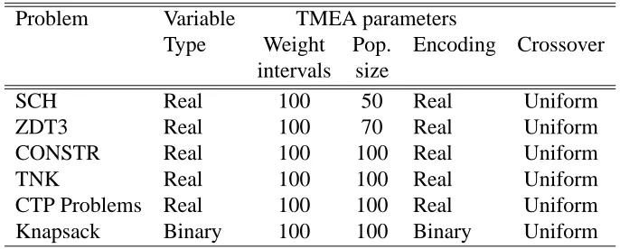
4.2 TMEA parameters and settings used in solving the test problems . . . 12
6.1 Accuracy comparison of TMEA with CMEA,NSGA-II, SPEA, and PESA
for different test problems. A larger value indicates a better performance . . 23
6.2 Spread comparison of TMEA with CMEA, NSGA-II, SPEA, and PESA
for different test problems. A larger value indicates better performance . . . 24
6.3 Coverage comparison of TMEA with CMEA, NSGA-II, SPEA, and PESA
for different test problems. A smaller value indicates better performance . . 25
A.1 Number of function evaluations for solving the test problems . . . 32
List of Figures
2.1 Illustration for a two objective problem . . . 4
2.2 Illustration for a two-objective problem with concave and convex non-inferior front . . . 5
2.3 Illustration for a two-objective problem with discontinuous non-inferior front 6 3.1 Flowchart for TMEA . . . 9
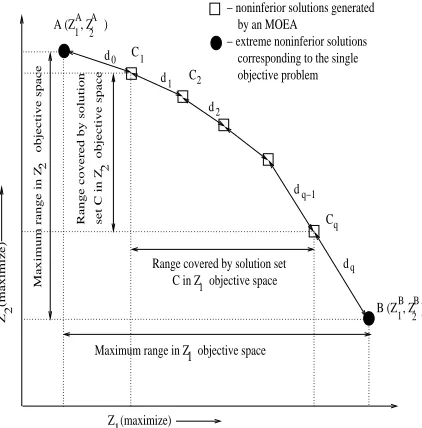
5.1 An example two-objective nondominated tradeoff to illustrate the compu-tation of Spread and Coverage metrics. . . 14
6.1 Non dominated solutions for the F2 problem . . . 16
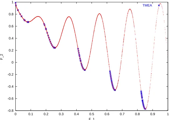
6.2 Non dominated solutions for the ZDT3 problem . . . 16
6.3 Non dominated solutions for the CONSTR problem . . . 17
6.4 Non dominated solutions for the SRN problem . . . 18
6.5 Non dominated solutions for the TNK problem . . . 18
6.6 Non dominated solutions for the CTP2 Problem . . . 19
6.7 Non dominated solutions for the CTP3 Problem . . . 20
6.8 Non dominated solutions for the CTP7 Problem . . . 20
6.9 Non dominated solutions for the CTP6 Problem . . . 21
6.10 Non dominated solutions for the Multiobjective Knapsack Problem . . . 21
Chapter 1
Introduction
Most real world engineering optimization problems require consideration of more than one
objective. These objectives portray diverse design criteria and are often conflicting. The
goal in single objective optimization is to find the best solution with respect to the
objec-tive considered. In multiobjecobjec-tive optimization the goal is to find a set of non-dominated
solutions (also called the Pareto optimal set) that represent the non-inferior tradeoff among
the multiple objectives being considered.
The concept of Pareto optimum was formulated by Vilfredo Pareto in 1896 [6] and is
considered as the origin of research in multiobjective optimization. Several mathematical
programming approaches like the -constraint method [3], Compromise programming [19],
Min-Max techniques [1], Goal programming [4] emerged during the first half of the
twenti-eth century. The Tchebycheff interactive vector space reduction mtwenti-ethod has been
success-fully used in the mathematical programming for a variety of applications [22].
As evolutionary algorithms (EAs) continue to be used in solving real world
optimiza-tion problems and show promise for successful applicaoptimiza-tion in a variety of domains
ar-eas [9], interest in extending their capabilities to multiobjective analysis is rapidly
grow-ing. Since the development of the Vector Evaluated Genetic Algorithm (VEGA) by
Schaf-fer [23], there has been a growing interest in the use EAs for solving multiobjective
op-timization problems (MOPs). The state-of-the-art in multiobjective evolutionary
algo-rithms (MOEAs) is well represented by Deb [10] and Coello Coello et al [7]. The more
Chapter 1. Introduction 2
commonly cited among them are the Nondominated Sorting Genetic Algorithm
(NSGA-II) [12], Strength Pareto Evolutionary Algorithm (SPEA-(NSGA-II) [27], Multiobjective Genetic
Algorithm (MOGA) [15], Niched Pareto Genetic Algorithm (NPGA) [17]. All these
tech-niques are termed as Pareto based approaches [16] i.e., they converge towards the Pareto
front in a single execution of the algorithm. These techniques mainly differ in the way they
assign fitness to the individuals within a population. Alternatively, there is a class of EAs
that generates the Pareto front by iteratively solving a series of single objective optimization
problems. The -constraint method-based evolutionary algorithm (CMEA) [20] [21] and
Subdivision Method [2] fall into this class. These algorithms generate comparable results
to the population-based searches and are relatively easier to implement.
This paper presents a new MOEA that utilizes the Tchebycheff method iteratively to
generate a set of non-dominated solutions. It uses the concepts of beneficial seeding [20]
to improve convergence during the intermediate iterations of the algorithm. It is tested
us-ing standard test problems havus-ing convex, concave and discontinuous Pareto surfaces, and
evaluated using several performance metrics commonly reported in the MOEA literature.
Its performance is compared with that of CMEA and other population based search
algo-rithms.
The next section describes the mathematical foundation for the Tchebycheff method,
fol-lowed by a description of the new EA-based approach. Descriptions of test problems,
re-sults, and performance comparisons of the new algorithm with other contemporary MOEAs
Chapter 2
The Tchebycheff Method
The Tchebycheff method is an iterative algorithm where preference information from the
decision maker is taken progressively as the algorithm proceeds to find a set of
non-dominated solutions. The preference information is characterized via two user-specified
inputs. One is an utopian objective vector or ideal solution ( ) to the MOP, and the
other is a weight vector ( ; ! #"$ &%'%(%( # ) that assigns user’s relative preference for the
objectives. The algorithm then proceeds to find the non-dominated solution that is closest
to by solving the following mathematical model.
Minimize )+*
',-,-./10 $32-4
5
627 (2.1)
Subject to 8&9
;:=<>9?@ A #" &%(%'%( CB (2.2)
DFEHG
/
2DIEKJL:> M AN (2.3)
O
QP&/
D@ (2.4)
ER
where, is one of the -objectives being maximized and
is the corresponding
4SUT
utopian objective vector value, isSUT weight from the weight vector. 8V9
W
is theX1SUT
con-straint for the original problem, B is the total number of the constraints,
represents the
decision vector and R represents the decision space. Most often is defined by
incre-menting each individual optimumYL
[Z
by an arbitrarily small amount\6]J^_= ! #" M%'%(%' `]N .
Chapter 2. The Tchebycheff Method 4
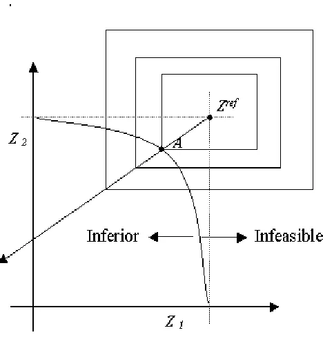
Figure 2.1: Illustration for a two objective problem
Figure 2.1 shows for an illustrative two objective case, different contours of the
Tcheby-cheff metric (2.1) for a given set of . The innermost rectangle represents the minimum
contour, and the optimal solution to the above model is point A. As no feasible solution
is present in the northeast quadrant (for the maximization problem), no other solution can
dominate this optimal solution. Thus, solution A found by solving model (1)-(2), by
defi-nition, is a non-dominated solution.
A different weight vector will result in a different set of rectangular contours and a
corresponding new optimal solution, yielding another non-dominated solution. By varying
JVD4N and solving model (1)-(2), different non-dominated solutions are generated until the
decision maker is satisfied with a solution. Alternatively, this procedure can be applied to
estimate the entire noninferior tradeoff among the objectives by iterating through the full
range of values for the weight vector.
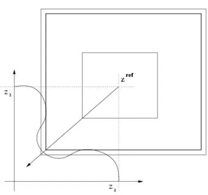
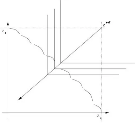
Chapter 2. The Tchebycheff Method 5
Pareto front is convex and concave in shape, discontinuous, or discrete. A few examples
are illustrated in Figures 2.2 and 2.3
Figure 2.2: Illustration for a two-objective problem with concave and convex non-inferior
Chapter 2. The Tchebycheff Method 6
Chapter 3
Tchebycheff Method-based EA
For engineering problems where the Tchebycheff formulation of the multiobjective
op-timization model (1)-(2) cannot be solved using a mathematical programming approach,
heuristic search procedures, including evolutionary algorithms, can be applied. The
Tcheby-cheff method-based evolutionary algorithm (TMEA) presented in this paper is a procedure
that integrates the above Tchebycheff method within an evolutionary computation
frame-work.
TMEA is described here in the context of generating the entire non-inferior tradeoff.
Starting at an extreme of the non-inferior set, this procedure solves the model (1)-(2)
corre-sponding to that weight vector via an evolutionary algorithm. This weight vector is
incre-mentally changed and the updated model is resolved to find adjacent non-inferior points,
eventually exploring the entire non-inferior space.
This procedure can become computationally intensive as it involves solving a series
of single objective problems. TMEA uses the concepts of beneficial seeding to improve
convergence within the intermediate iterations by seeding the starting solutions with the
converged solutions obtained in the previous generations. This not only achieves faster
convergence but also improves the search. This method was successfully implemented
within the CMEA approach for multiobjective optimization [20].
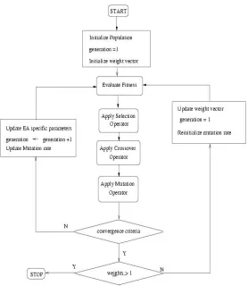
The flowchart in Figure 3.1 shows the sequence of execution of the algorithm. The
inner loop of the flow chart corresponds to the execution of any EA with typical operators
Chapter 3. Tchebycheff Method-based EA 8
like selection, recombination and mutation. The stopping criterion for the inner loop is
determined either by exceeding maximum generations or a specified number of generations
without improvement in the best solution. The outer loop of the flow chart corresponds
to the change in the vector. From Equation 2.1 this corresponds to a shift in the weight
placed on the objectives and consequentially a change in the direction of the search process.
The number of non-dominated solutions being obtained depends on the step-size chosen for
incrementing the vector. For each execution of the outer loop, the EA in the inner loop
solves a particular instance of the problem described by Equations (1)-(2) and generates a
non-inferior solution. After each execution of the outer loop, the vector is incremented.
The solutions generated through sequential execution of the outer loop will represent the
non-dominated (or Pareto optimal) set.
An adaptive mutation parameter defined in Equation 3.1 is used to introduce higher
diversity at the start of a new iteration of the outer loop. The mutation operator is applied
adaptively, starting with a higher rate initially and reducing it exponentially as generations
proceed in the inner loop. The higher rate at the beginning increases the diversity in the
previously converged population of solutions potentially avoiding premature convergence.
Mutation Rate
a
bdc
:>%( if
e
@
Max
:>%f:> ! `:%' hgji#kl
5 e3m V: 3 nVe3oqp&rLs t p (3.1) where e
Chapter 3. Tchebycheff Method-based EA 9
Chapter 4
Evaluation of TMEA
Apart from the development of newer and improved algorithms for MOPs, researchers have
also concentrated on developing test functions to validate and test MOEAs. Veldhuizen [25]
summarized many test functions that have been suggested by different researchers. Deb et
al [11] presented the Tunable Test Problem generator that can be used to generate problems
of varying complexity, and Deb et al [13] suggested a test suite of MOPs with more than
two objectives. More recently Knowles and Corne [8] introduced a test suite based on the
Quadratic Assignment Problem (QAP).
The TMEA was tested on the following test problems, each with different degrees of
difficulty and different characteristics with respect to convexity and continuity in the
non-inferior set, discreteness in the decision space, and degree of constraints. The set of
con-strained test problems (CTPs) by Deb [11], the extended 0/1 knapsack problem presented
by Zitzler [27] and two of the commonly used unconstrained test problems are used to test
TMEA. A complete list and details of the test problems that were used in this study is
pro-vided in Table 4.1. The parameter settings used for all the algorithms is propro-vided in the
Table 4.2. All objective and constraint functions values were normalized, and
correspond-ingly the weight values were kept to a [0, 1] range. The constraints, where applicable,
were handled using the constraint violation-based selection approach suggested by Deb et
al [12]. Each test function was solved for a 50 random trials to test the robustness of the
algorithm.
Chapter 4. Evaluation of TMEA 11
Table 4.1: Test problems used in this study. The objective functions are denoted by?uW
,
v w , where denotes the number of objectives and the number of decision
variables.
Problem N Domain Objective Functions Constraints
CONSTR 2 x]yz|{}!~U _yQx IKxqy yQx IKx>FMxqy
x z|{}![ Qx IvHx x y Qx Ix Mx y
SRN 2 x z|{&}![&}M _yQx IvQxqyF^
yQx IKx y Hx VV Qx CVQx IKx]yF|Mx `} &[ ¡VQx I¢MxqyFQx£
TNK 2 x z|{}!¥¤> _yQx IKxqy yQx Ix
y ¦x ¢H}!~U C§V¨©#&ª©«V3¬ª©FQxqy6x }
&[ ¡VQx IKx CVQx IvQx]yFw}!~®^
Qx¯w}!~®^ }!~®
SCH 1 x z|{A3° _yQx IKx
Unconstrained
&[ Qx IvQx±|^
ZDT3 30 x]yz|{}!#6 _yQx IKxqy
x ²} Qx I³>Qx C{´ xµ³>Qx Unconstrained
xµ³>Qx ¨ F`}V¤y# ¢A`~¶~¶~¶ ³>Qx I1·¢¸ U¹
x !Qº£
Knapsack 750 »}!#M¼M½
Qx I · ¸ 93¹ y&¾
.96x 9 · ¸
96¹ y!¿
.9
Problem À>Áq&[A`~¶~¶~¶[Â x 9
CTP 5 x]yz|{}!#6 _yQx IKxqy VQx Iâ6§V¨AÅÄ© C¡^Qx µ|Æ
Problem x z|{A~U#A[A~U# Qx I³>Qx CÇDÈÉfÊË
Ì
ÉÍÊË
¨
FÅÄ© y x ¯£ªÎ¨
FWÏ6¤
¢A`~¶~¶~¶ ³>Qx I`}& W¨
FÅÄ© C¡VQx Ð|Æ ·K¸ U¹ y Qx
£`}VC§V¨AW&¤x C§V¨©ÅÄA _yQx 4Ñ[ `ÎÒ
CTP2:ÄÓv}!~®&¤ ,ªh²}!~® ,Ï`} ,v ,Ôh¢ ,ÆÕ
CTP3:ÄÓv}!~®&¤ ,ªh²}!~U ,Ï`} ,v ,Ôh²}!~® ,ÆÖ
CTP6:ÄÓ¢}!~U`¤ ,ªhK×^} ,ϲ}!~® , ,ÔØ¢ ,Æ
Chapter 4. Evaluation of TMEA 12
Table 4.2: TMEA parameters and settings used in solving the test problems
Problem Variable TMEA parameters
Type Weight Pop. Encoding Crossover
intervals size
SCH Real 100 50 Real Uniform
ZDT3 Real 100 70 Real Uniform
CONSTR Real 100 100 Real Uniform
TNK Real 100 100 Real Uniform
CTP Problems Real 100 100 Real Uniform
Chapter 5
Performance Assessment
The results generated by TMEA and other MOEAs are compared with respect to three
performance metrics: accuracy, spread, and coverage.
Ù
AccuracyÚ This metric is used to compare the degree of dominance of the
non-dominated set of solutions obtained by one method over those obtained
by another. The S-factor defined by Zitzler and Thiele [26] is computed to
characterize this metric in the comparisons made in this paper. For a set of
maximization objectives, a larger value represents a better performance. A
more detailed description about the S-factor with proofs can be found in [14].
Ù
SpreadÚ This metric is used to compare how much of the range of the
non-inferior surface is covered by a set of non-dominated solutions. The spread
parameter reported by Chetan [5] and Ranjithan et al. [20] is used to
character-ize this metric in the comparisons made in this paper. Using the illustration in
Figure 5.1, points A and B refer to the two extreme noninferior solutions
(cor-responding to the single objective optima for each objective). The maximum
range covered by the MOEA generated non-dominated solutions represented
by the ordered setÛÜÝJLÛ
T
[<
o
EKJD ! M%'%( CÞDN1N is 4àßAá y 5 ß È y and4 ß È 5 âßAá in
y and objective space, respectively. The spread metrics in objective space
y and are defined as
4àßAá y 5 ß È y 3m4àã y 5 Óä y and 4 ß È 5 âßAá 6muâä 5 âã ,
respectively. A larger value of this metric indicates better performance.
Chapter 5. Performance Assessment 14
Ù
CoverageÚ This metric is used to compare how well the non-dominated
solu-tions obtained by an MOEA are distributed in the objective space. Coverage
is calculated by measuring the Euclidean distance between adjacent solutions
to measure the distribution in objective space. Two coverage metrics V1 and
V2 are defined ([5],[20]) to characterize the coverage within the range of
non-inferior region defined by (1) the extreme nonnon-inferior solutions A and B, and
(2) by the extreme solutions (Û y and Ûå ) generated by that MOEA,
respec-tively. Using the notations from Figure 5.1, V1 is defined as )+*
JLæ T [< o E
JL:> M ! &%(%'%( CÞDN1N , and V2 is defined as )+*
JLæ
T
[<
o
EvJD ! &%(%(%' CÞ
5
AN1N . A smaller
value of V1 (or V2) implies more closely spaced noninferior solutions, thus
indicating better coverage.
Z (maximize) 2
Maximum range in Z objective space
2
A (Z , Z )A
1 2 A
Z (maximize) 1
Maximum range in Z objective space1 d d d d d 0 1 2 q−1 q C C C 1 2 q
C in Z objective space Range covered by solution set
1
set C in Z objective space
2
Range covered by solution
B (Z , Z )
1 2 B B
)
− noninferior solutions generated by an MOEA
− extreme noninferior solutions corresponding to the single objective problem
Figure 5.1: An example two-objective nondominated tradeoff to illustrate the computation
Chapter 6
Results
For the test problems summarized in Table 4.1, the sets of non-dominated solutions
tained using TMEA are presented in graphs showing the non-inferior surface in the
ob-jective space. While the results were generated for 50 random trials, the results for only
a representative run are reported here since the results exhibited robust behavior. Where
available, non-dominated solutions reported in the literature are also shown for comparison.
Further these solutions are compared using the performance metrics described above.
6.1
Unconstrained Test Problems
Schaffer’s F2 problem [23] and the ZDT3 [13] problem are two unconstrained test
prob-lems that were used to evaluate TMEA. While F2 problem represents a continuous Pareto
surface, the ZDT3 problem consists of discontinuities. The sets of non-dominated solutions
obtained using TMEA are shown in Figures 6.1 and 6.2.
6.2
Constrained Test Problems with Continuous Decision
Variables
Several constrained problems with continuity in the decision space were used to evaluate
TMEA. Figures 6.3 and 6.4 show the non-dominated solutions obtained by TMEA for the
Chapter 6. Results 16
0 0.5 1 1.5 2 2.5 3 3.5 4
0 0.5 1 1.5 2 2.5 3 3.5 4
F_2
F_1
TMEA
Figure 6.1: Non dominated solutions for the F2 problem
-0.8 -0.6 -0.4 -0.2 0 0.2 0.4 0.6 0.8 1
0 0.1 0.2 0.3 0.4 0.5 0.6 0.7 0.8 0.9 1
F_2
F_1
TMEA
Chapter 6. Results 17
Figure 6.3: Non dominated solutions for the CONSTR problem
CONSTR problem and the SRN problem, both described by Deb et al [11].
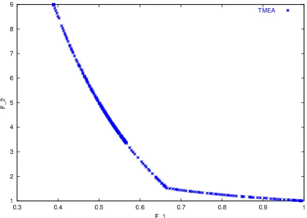
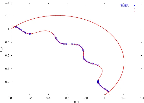
Figure 6.5 shows the non-dominated solutions for the TNK problem that was proposed
by Tanaka [24]. While the Pareto fronts for the CONSTR and SRN problems are continuous
in the objective space, the Pareto front for the TNK problem includes discontinuities. In all
these cases, the results indicate that TMEA was able to generate non-dominated solutions
that represent the true Pareto front accurately with a uniform coverage.
The following set of constrained test problems (CTP2, CTP3, CTP6, and CTP7) was
used to compare the results obtained using TMEA with those obtained using other MOEAs.
Different instances of CTP, representing sharp discontinuities in the objective space, were
proposed by Deb et al [11], and have been used frequently in testing and comparisons in
the MOEA literature. The Figures 6.6 - 6.8 show the solutions obtained by TMEA for the
CTPs along with those obtained by NSGA-II and CMEA. The results for NSGA-II and
CMEA are obtained from the results reported by Kumar [18].
The Pareto front for CTP2 has a number of discontinuous regions, making the search
Chapter 6. Results 18
-300 -250 -200 -150 -100 -50 0 50 100 150 200
0 50 100 150 200 250 300
F_2
F_1
TMEA
Figure 6.4: Non dominated solutions for the SRN problem
0 0.2 0.4 0.6 0.8 1 1.2 1.4
0 0.2 0.4 0.6 0.8 1 1.2 1.4
F_2
F_1
TMEA
Chapter 6. Results 19
0.2 0.4 0.6 0.8 1 1.2
0 0.2 0.4 0.6 0.8 1
F_2
F_1
TMEA CMEA NSGA-II
Figure 6.6: Non dominated solutions for the CTP2 Problem
in the Figure 6.6, TMEA was able to find successfully non-dominated solutions in all the
disconnected regions. For this problem, TMEA performs relatively well in comparison to
the solutions obtained by the other algorithms. The performance metrics are compared in
Tables 6.1, 6.2 and 6.3.
CTP3 and CTP7 (Figures 6.7 - 6.8) consist of discrete regions in the Pareto front where
one solution represents the non-inferior solution in each discontinuous region. For CTP3
(Figure 6.7), TMEA performs well to identify a non-dominated solution in each discrete
region, but does not do as well as CMEA in several regions.
For CTP7 (Figure 6.8), TMEA again is able to identify non-dominated solutions in
sev-eral of the discrete regions, and does better than the other algorithms in those regions. It
misses, however, to identify non-dominated solutions in all discrete regions while CMEA
was able to have a better distribution of non-dominated solutions. Again, the numeric
val-ues of the performance metrics are compared in Tables 6.1, 6.2 and 6.3. CTP6 (Figure 6.9)
represents a problem with discrete bands of feasible regions in the objective space with one
Chapter 6. Results 20
0.2 0.4 0.6 0.8 1 1.2
0 0.2 0.4 0.6 0.8 1
F_2
F_1
TMEA CMEA NSGA-II
Figure 6.7: Non dominated solutions for the CTP3 Problem
-1 0 1 2 3 4 5
0 0.1 0.2 0.3 0.4 0.5 0.6 0.7 0.8 0.9 1
F_2
F_1
TMEA CMEA NSGA-II
Chapter 6. Results 21
0 2 4 6 8 10 12
0 0.2 0.4 0.6 0.8 1
F_2
F_1
TMEA CMEA NSGA_II
Figure 6.9: Non dominated solutions for the CTP6 Problem
Chapter 6. Results 22
this problem.
6.3
Constrained Test Problem with Discrete Decision
Vari-ables
Performance of TMEA was also tested and compared using the extended multiobjective
knapsack problem proposed by Zitzler and Thiele [26]. This is a constrained problem with
binary decision variable with a Pareto front as shown in Figure 6.10. This problem was
been solved for two objectives with 500 items and 750 items. The results reported here
correspond to 750 items and two knapsacks. The results are compared with those obtained
from the CMEA and a Binary Linear Programming (BLP) solver that was solved using
CPLEX. The BLP solution represent the best available estimation of the Pareto front.
Non-dominated solutions obtained using TMEA compare well with respect to the BLP solution,
and perform relatively better than the solutions obtained using CMEA. The performance
metrics compared in Tables 6.1, 6.2 and 6.3 show the superior performance of TMEA with
Chapter 6. Results 23
Table 6.1: Accuracy comparison of TMEA with CMEA,NSGA-II, SPEA, and PESA for
different test problems. A larger value indicates a better performance
The MOEAs Compared Problem (ç y ,ç ): (ç factor for)+èêéêë y data set,
()+èéìë y vs)+èéìë ) instance ç factor for )+èéìë data set)
(TMEA vs NSGA-II) CTP2 (0.613, 0.6075)
(TMEA vs CMEA) CTP2 (0.613, 0.6123)
(TMEA vs NSGA-II) CTP3 (0.578, 0.5823)
(TMEA vs CMEA) CTP3 (0.578, 0.5931)
(TMEA vs CMEA) CTP6 (0.525, 0.560)
(TMEA vs NSGA-II) CTP6 (0.525, 0.5663)
(TMEA vs NSGA-II) CTP7 (0.512, 0.1543)
(TMEA vs CMEA) CTP7 (0.512, 0.6563)
(TMEA vs NSGA-II) Knapsack (0.731, 0.623)
(TMEA vs CMEA) Knapsack (0.731, 0.707)
(TMEA vs PESA) Knapsack (0.731, 0.602)
Chapter 6. Results 24
Table 6.2: Spread comparison of TMEA with CMEA, NSGA-II, SPEA, and PESA for
different test problems. A larger value indicates better performance
The MOEAs Compared Problem ( spread for)+èêéêë y , ( " spread for)+èêéêë y ,
()íèéêë y vs)íèéêë ) instance spread for )+èéìë ) " spread for )íèéêë )
(TMEA vs NSGA-II) CTP2 (1.000, 1.000) (0.997, 1.000)
(TMEA vs CMEA) CTP2 (1.000, 1.000) (0.997, 1.000)
(TMEA vs NSGA-II) CTP3 (0.991, 0.996) (1.000, 1.000)
(TMEA vs CMEA) CTP3 (0.991, 0.997) (1.000, 1.000)
(TMEA vs NSGA-II) CTP6 (0.967, 0.974) (0.934, 0.973)
(TMEA vs CMEA) CTP6 (0.967, 0.999) (0.934, 1.000)
(TMEA vs NSGA-II) CTP7 (0.755 , 0.036) (0.510, 0.234)
(TMEA vs CMEA) CTP7 (0.755, 0.989) (0.510, 1.000)
(TMEA vs NSGA-II) Knapsack (1.000, 0.269) (0.925, 0.269)
(TMEA vs CMEA) Knapsack (1.000, 0.922) (0.925, 0.920)
(TMEA vs PESA) Knapsack (1.000, 0.280) (0.925, 0.261)
Chapter 6. Results 25
Table 6.3: Coverage comparison of TMEA with CMEA, NSGA-II, SPEA, and PESA for
different test problems. A smaller value indicates better performance
The MOEAs Compared Problem (î for)+èéìë y ,îï for (î" for)+èêéêë y ,îê" for
()íèéêë y vs)íèéêë ) instance )+èéìë ) (includes the )+èéìë ) (excludes the
known extreme points known extreme points
for each objective) for each objective)
(TMEA vs NSGA-II) CTP2 (0.074, 0.350) (0.262, 0.102)
(TMEA vs CMEA) CTP2 (0.074, 0.096) (0.262, 0.096)
(TMEA vs NSGA-II) CTP3 (0.142, 0.360) (0.165, 0.133)
(TMEA vs CMEA) CTP3 (0.142, 0.171) (0.165, 0.161)
(TMEA vs NSGA-II) CTP6 (0.053, 0.038) (0.070, 0.035)
(TMEA vs CMEA) CTP6 (0.053, 0.152) (0.070, 0.091)
(TMEA vs NSGA-II) CTP7 (0.222, 1.590) (0.999, 0.007)
(TMEA vs CMEA) CTP7 (0.222, 0.424) (0.999, 0.4249)
(TMEA vs CMEA) Knapsack (0.082, 0.089) (0.082, 0.066
(TMEA vs PESA) Knapsack (0.082, 0.674) (0.082, 0.010)
Chapter 7
Summary and Conclusions
This paper describes TMEA, a new EA-based multiobjective optimization procedure that
builds upon the Tchebycheff method. Tchebycheff method has been established before
and solved using mathematical programming procedures to estimate the non-inferior
so-lutions for multiobjective optimization problems. The convergence of TMEA is enhanced
by beneficial seeding of the population within the subiterations of the algorithm, a notion
borrowed from mathematical programming-based MO analysis. Unlike other commonly
reported MOEAs that attempt to converge the population of solutions simultaneously to
the non-inferior set, TMEA attempts to converge first the population of solutions to an
ex-treme inferior solution and then incrementally migrate the population to trace the
non-inferior surface. As no new algorithm-specific operators or special encoding are needed,
the structure of the algorithm enables easy integration with existing implementation of EAs
for an optimization problem. This is important when analyzing large-scale realistic
prob-lems for which much effort is already spent on configuring and implementing the base
evolutionary algorithms.
TMEA was evaluated by applying it to a number of test problems with different
char-acteristics and levels of difficulty. This evaluation included problems involving continuous
as well as combinatorial decision space, unconstrained as well as constrained
optimiza-tion, real as well as binary variables, and concave as well as convex Pareto optimal sets.
To characterize the performance of the algorithms, metrics quantifying accuracy, spread,
Chapter 7. Summary and Conclusions 27
and coverage were used. Solutions were generated for several different random seeds, and
TMEA showed robust behavior in generating the non-dominated solutions. Overall, TMEA
performed relatively well with respect to these criteria and for the different problems tested.
By exploring specific regions of the objective space through different combinations of
the weights in TMEA, the coverage and spread of the noninferior solutions are enforced
explicitly and independent of noninferiority, resulting in excellent coverage while
perform-ing well with respect to noninferiority. While this approach can yield a relatively uniform
coverage of the non-inferior region, depending on the shape of the Pareto front it is
pos-sible to converge to the same non-dominated solution for different weights, resulting in
potential inefficiencies.
Further testing is needed to evaluate the effectiveness of applying TMEA to
higher-order MO problems. As the number of objectives increases, the number of weight
vec-tors increase, requiring increases in the combinatorial combinations of these weights. The
computational as well as convergence performances associated with scale-up in the
prob-lem dimension need to be examined. TMEA is currently being applied to a real-world
water resources management problem that requires MO analysis. The practicality of such
References
[1] Balling, R. J. Pareto sets in decision-based design. Journal of Engineering Valuation
and Cost Analysis, 3:189–198, 2000.
[2] Dornberger, R. and B¨uche, D. New evolutionary algorithm for multi-objective
op-timization and the application to engineering design problems. In Proceedings of
the Fourth World Congress of Structural and Multidisciplinary Optimization, Dalian,
China, 2001. International Society of Structural and Multidisciplinary Optimization
(ISSMO).
[3] Chankong, V. and Haimes, T. T. Multiobjective Decision Making: Theory and
Methodology. North-Holland, New York, 1983.
[4] Charnes, A., Cooper, W. and Ferguson, R. Optimal estimation of executive
compen-sation by linear programming. Management Science, 1:138–151, 1955.
[5] Chetan, S. K. Noninferior surface tracing evolutionary algorithm (NSTEA) for
mul-tiobjective optimization. Master’s thesis, North Carolina State University, Raleigh,
NC., 2000.
[6] Carlos, A. C. C. An updated survey of evolutionary multiobjective optimization
tech-niques: State of the art and future trend. In Peter J. Angeline, Zbyszek Michalewicz,
Marc Schoenauer, Xin Yao, and Ali Zalzala, editors, Proceedings of the Congress on
Evolutionary Computation, pages 3–13. IEEE press, 1999.
References 29
[7] Carlos, A. C. C., Van Veldhuizen, David, A. and Lamont, Gary, B. Evolutionary
Al-gorithms for Solving Multi-Objective Problems. Kluwer Academic Publishers, New
York, 2002.
[8] Corne, D. W. and Knowles, J. D. Instance Generators and Test Suites for the
Mul-tiobjective Quadratic Assignment Problem In Carlos M. Fonseca, Peter J.
Flem-ing, Eckart Zitzler, Kalyanmoy Deb, and Lothar Thiele, editors, Evolutionary
Multi-Criterion Optimization. Second International Conference, EMO 2003, pages 295–
310, Faro, Portugal, April 2003. Springer. Lecture Notes in Computer Science.
Vol-ume 2632.
[9] Dasgupta, D. and Michalewicz, Z. Evolutionary Algorithms in Engineering
Applica-tions. Springer-Verlag, 1997.
[10] Deb, K. Multi-Objective Optimization Using Evolutionary Algorithms. Chichester,
UK : Wiley.
[11] Deb, K., Pratap, A. and Meyarivan, T. Constrained test problems for multi-objective
evolutionary optimization. In E. Zitzler et al., editor, Evolutionary Multi-Criteria
Op-timization 2001, Lecture Notes in Computer Science 1993, pages 284–298.
Springer-Verlag, 2001.
[12] Deb, K., Pratap, A. and Meyarivan, T. A fast and elitist multiobjective genetic
al-gorithm: NSGA-II. IEEE Transaction on Evolutionary Computation, 6(2):182–197,
April 2002.
[13] Deb, K., Thiele, L., Laumanns, M. and Zitzler, E. Scalable Test Problems for
Evo-lutionary Multi-Objective Optimization. Technical Report 112, Computer
Engineer-ing and Networks Laboratory (TIK), Swiss Federal Institute of Technology (ETH),
Zurich, Switzerland, 2001.
[14] Fleisher, M. The measure of pareto optima: Applications to multi-objective
References 30
and Lothar Thiele, editors, Evolutionary Multi-Criterion Optimization. Second
In-ternational Conference, EMO 2003, pages 519–533, Faro, Portugal, April 2003.
Springer. Lecture Notes in Computer Science. Volume 2632.
[15] Fonseca, C. M. and Fleming, P. J. Genetic algorithms for multiobjective optimization:
Formulation,discussion and generalization. In S. Forrest, editor, Proceedings of the
Fifth International Conference on Genetic Algorithms, pages 416–423, San Mateo,
California, 1993. Morgan Kaufmann.
[16] Fonseca, C. M. and Fleming, P. J. An overview of evolutionary algorithms in
multi-objective optimization. Evolutionary Computation, 3(1):1–16, 1995.
[17] Horn, J., Nafpliotis, N. and Goldberg, D. E. A niched pareto genetic algorithm for
multiobjective optimization. In Proceedings of the First IEEE Conference on
Evo-lutionary Computation,IEEE World Congress on Computational Computation,
vol-ume I, pages 82–87, Piscataway, NJ, 1994. IEEE Press.
[18] Kumar, S. V. Vitri - A Generic Framework for Engineering Decision Support Systems
on Heterogeneous Computer Networks. PhD thesis, North Carolina State University,
Raleigh, NC, January 2002.
[19] Zeleny, M. Compromise programming. In M.Zeleny J.L.Cochrane, editor, Multiple
Criteria Decision Making, pages 262–301, Columbia, South Carolina, 1973.
Univer-sity of South Carolina Press.
[20] Ranjithan, S. R., Chetan, S. K. and Dakshina, H. K. Constraint method-based
evolu-tionary algorithm (CMEA) for multiobjective optimization. In E. Zitzler et al., editor,
Evolutionary Multi-Criteria Optimization 2001, Lecture Notes in Computer Science
1993, pages 299–313. Springer-Verlag, 2001.
[21] Ranjithan, S. R. and Kumar, S. V. Evaluation of the constraint method-based
evolu-tionary algorithm (cmea) for a three-objective problem. In GECCO, pages 431–438.
References 31
[22] Steuer, R. E. Multiple Criteria Optimization: Theory, Computation and Applications.
John Wiley & Sons, Inc., 1986.
[23] Schaffer, D. J. Multiple objective optimization with vector evaluated genetic
algo-rithms. In J. J. Grefenstette, editor, Proc. of the First Int. Conf. on Genetic Algorithms,
pages 93–100, Hillsdale, NJ, 1985. Lawrence Erlbaum.
[24] Tanaka, M. Ga-based decision support system for multi-criteria optimization. In
Proceedings of the International Conference on Systems, Man and Cybernetics-2,
pages 1556–1561, 1995.
[25] Van Veldhuizen, D. A. Multiobjective Evolutionary Algorithms: Classifications,
Analyses, and New Innovations. PhD thesis, Department of Electrical and
Com-puter Engineering. Graduate School of Engineering. Air Force Institute of
Technol-ogy, Wright-Patterson AFB, Ohio, May 1999.
[26] Zitzler, E. and Thiele, L. Multiobjective evolutionary algorithms: A comparative
case study and the strength pareto approach. IEEE Transactions on Evolutionary
Computation, 2(4):257–271, 1999.
[27] Zitzler, E., Laumanns, M. and Thiele, L. SPEA2: Improving the Strength Pareto
Evolutionary Algorithm. Technical Report 103, Gloriastrasse 35, CH-8092 Zurich,
Appendix A
Computational Performance Evaluation of the
TMEA
Table A.1: Number of function evaluations for solving the test problems
Problem Num of Evaluations
First Iteration Avg for subsequent Total
iterations
Schaffer 2550 1400 141150
ZDT3 6550 3653 368185
CTP2 9494 4041 409460
CTP3 9560 3960 401670
CTP6 9952 3750 381233
CTP7 8724 3839 388785