Structure Learning and Classification in Complex Graphical Models

(1)

ABSTRACT

DU, XINGQI. Structure Learning and Classification in Complex Graphical Models. (Under the direction of Subhashis Ghoshal.)

Learning the structure of networks of random variables has received much attention. In this article, we investigate the properties and applications of complex graphical models to address two problems. The first problem involves a graphical model where a multi-variate normal vector is associated with each node of the underlying graph. We minimize a loss function obtained by regressing the vector at each node on those at the remaining ones under a group penalty. We show that the proposed estimator can be computed by a fast convex optimization algorithm. We show that as the sample size increases, the esti-mated regression coefficients and the correct graphical structure are correctly estiesti-mated with probability tending to one. By extensive simulations, we show the superiority of the proposed method over comparable procedures. We apply the technique on two real datasets. The first one is to identify gene and protein networks showing up in cancer cell lines, and the second one is to reveal the connections among different industries in the US.

(2)

(3)

(4)

Structure Learning and Classification in Complex Graphical Models

by Xingqi Du

A dissertation submitted to the Graduate Faculty of North Carolina State University

in partial fulfillment of the requirements for the Degree of

Doctor of Philosophy

Statistics

Raleigh, North Carolina 2018

APPROVED BY:

Sujit Ghosh Wenbin Lu

Eric Chi Subhashis Ghoshal

(5)

DEDICATION

(6)

BIOGRAPHY

(7)

ACKNOWLEDGEMENTS

First and foremost, I would like to express my deepest gratitude to my advisor, Dr. Sub-hashis Ghoshal, for his kind guidance, excellent inspiration and continued support. He helps me get started in statistical research, and patiently gives me advice and encourage-ment whenever I encounter difficulties. I am so lucky to have him as my advisor, without whom this disseration would not be possible.

I would like to thank Dr. Sujit Ghosh, Dr. Wenbin Lu and Dr. Eric Chi for taking precious time to serve on my Ph.D. committee. They have provided valuable comments that help me improve my work presented in this dissertation. I also thank Dr. Min Kang from the Department of Mathematics for attending my defense as the graduate school representative.

I appreciate the study resources provided by the Department of Statistics at North Carolina State University. I am grateful for all the faculty members for providing a friendly environment and broadening my knowledge in the world of statistics. I thank Dr. Eric Laber for being my academic advisor during my first two years study. Special thanks to all my friends who support and encourage me as always.

I am also thankful to the internship experiences at Pfizer and SAS. Special thanks to my supervisors, Kosalaram Goteti, Yolanda Ingram, Michael Leonard and Jerzy Brzezicki for sharing with me many practical knowledge and skills.

(8)

LIST OF TABLES

Table 2.1 Model selection comparison withpthe number of nodes,qthe number of true edges andnthe sample size with the tuning parameterλoptimized by cross-validation. Cases considered below are (i)p= 30,q= 177 (41% density) (ii) p= 50, q = 137 (11% density), (iii) p= 100, q = 419 (8% density), (iv) p= 200, q= 617 (3% density), (v) p= 400, q= 782 (1% density) where the density is 100q/ p₂ in percentage. . . 21 Table 2.2 Summary statistics for protein, gene and gene-protein networks . . . . 41 Table 2.3 Top 20 most connected nodes for three networks (sorted by decreasing

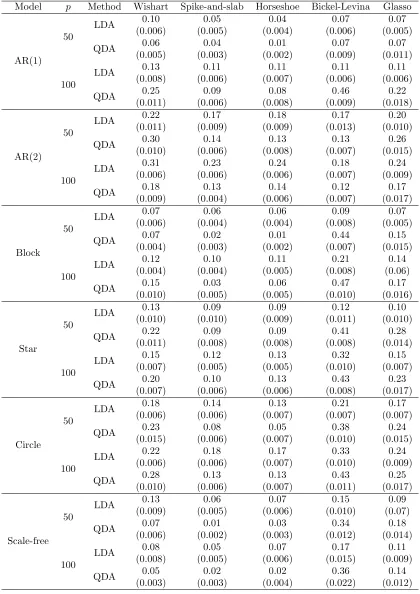
degrees) . . . 41 Table 3.1 Misclassification rates for normally distributed data with standard

er-rors (se) in parentheses in LDA setting (n= 100) . . . 61 Table 3.2 Misclassification rates for t-distributed data with standard errors (se)

in parentheses in LDA setting (n = 100) . . . 62 Table 3.3 Misclassification rates for normally distributed data with standard

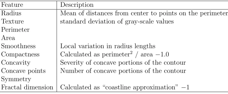
er-rors (se) in parentheses in QDA setting (n = 100) . . . 64 Table 3.4 Ten features computed for each cell nucleus . . . 66 Table 3.5 Prediction errors using 5-fold cross-validation for the breast data

anal-ysis with estimated standard errors in parentheses . . . 66 Table 4.1 Misclassification rates for normally distributed data with standard

(10)

LIST OF FIGURES

Figure 2.1 Estimation accuracy comparison: total detected edges vs. correctly detected edges with 190 true edges (44%): (a) K = 3; (b) K = 5; (c) K = 8 . . . 17 Figure 2.2 Estimation accuracy comparison: total detected edges vs. correctly

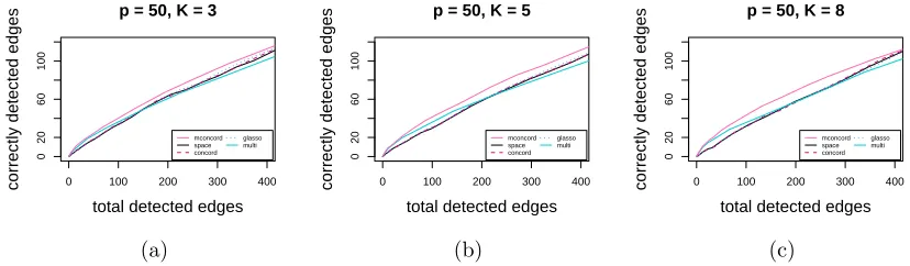
detected edges with 262 true edges (21%): (a) K = 3; (b) K = 5; (c) K = 8 . . . 17 Figure 2.3 Estimation accuracy comparison: total detected edges vs. correctly

(11)

Chapter 1 Introduction

Finding structural relations in a network of random variables (Xi : i ∈V) is a problem

of significant interest in modern statistics, and can be applied to many machine learning problems. A graphical model describes the intrinsic dependence between variables, where two nodesi, j ∈V are connected by an edge if and only if the two corresponding variables

Xi and Xj are conditionally dependent given all other variables. Under the assumption

that variables follow multivariate normal distributions, the conditional independence be-tween the variable located at node i and that located at node j is equivalent of having zero at the (i, j)th entry of the precision matrix Ω = Σ−1_{. Therefore, the problem of}

(12)

the application of a full Bayesian method for classification.

Under the first framework, it is natural to learn the sparse structure using regulariza-tion method with a lasso-type penalty. A large number of works addressed estimaregulariza-tion of network structure where a univariate variable is associated with a node of the underlying network. For example, Friedman et al. [13] and Banerjee et al. [1] proposed the graphical lasso, and its convergence property was studied by Rothman et al. [35]. A closely related method was proposed by Yuan & Lin [41]. A more scalable alternative where the pseudo-likelihood instead of the actual pseudo-likelihood is obtained was pioneered by Meinshausen & B¨uhlmann [32]. Peng et al. [34] improved the method by taking symmetry of the precision matrix into account, and a weighted version of it was considered by Khare et al. [20].

However, the above approaches are designed for problems where all variables are uni-variate. In many situations, such as if multiple characteristics are measured, the variables

Xi at different nodes i ∈ V may be multivariate. One possible solution is to treat each

component of these variables as separate one-dimensional variables, but the group infor-mation is ignored. The multivariate network problem is addressed by Kolar et al. [21], who pursued a likelihood based approach, where the computation is a big challenge, especially when the number of variables at each node increases.

In Chapter 2, we extend the work of Khare et al. [20] to the multivariate setting and formulate a multivariate analog based on a regression based pseudo-likelihood. Similar to the univariate case, this approach is computationally more efficient than the likelihood based method. Its performance is addressed by simulation studies and is applied in two real data applications. We also study large sample properties of the proposed method.

(13)

class classification, which relies on a simple application of the Bayes theorem. The key point for higher classificaiton accuracy is to get a good estimate of the precision matrix. In the high dimensional setting, it is reasonable to assume that the precision matrix is sparse, meaning that only a few intrinsic relations exist among variables. Many frequen-tist approaches have been proposed to estimate the precision matrix Ω or the covariance matrix Σ, as in Huanget al. [17], Ledoit and Wolf [22], Bickel and Levina [6, 7], and Cai

et al.[8, 9]. There are also several methods in the frequentist literature for the estimation of the precision matrix through graphical models, as mentioned earlier in this chapter.

Bayesian methods for inference using graphical models have also been developed. Wishart prior is a natural choice in the Gaussian setting, but it is not desirable for high-dimensional data, since no sparsity is incorporated. Banerjee and Ghosal [2] considered a conjugate graphical Wishart prior which could be applied to high-dimensional setting. Wang [39] introduced Bayesian graphical lasso that requires a forceful restriction to the cone of positive definite matrices. Banerjee and Ghosal [3] modified the Bayesian graphical lasso to allow point mass on the prior for off-diagonal entries, and used a Laplace approximation technique to avoid MCMC methods for large samples. A major challenge of priors using a combination of point mass and a continuous density is the computational burden. A spike-and-slab prior (Mitchell and Beauchamp [33], George and McCulloch [14], Ishwaran and Rao [18]) uses a normal distribution with very small variance to replace the point mass, and a faster computing algorithm was recently developed by Ro˘ckov´a and George [36].

(14)

In Chapter 3, we consider a Bayesian method for two-class classification. In order to guarantee the positive-definiteness of the precision matrix wihout imposing further restrictions, we put priors on the Cholesky decomposition of the precision matrix. We put sparse priors using spike-and-slab or horseshoe priors on the off-diagonal entries. The detailed posterior calculation on both priors is provided. Rates of contractions of the posterior distributions of model parameters are also derived. The empirical performance of the proposed approach is evaluated by simulations and illustrated with an application to a breast cancer dataset.

(15)

Chapter 2 Multivariate Gaussian Network

Structure Learning

2.1 Introduction

Finding structural relations in a network of random variables (Xi : i ∈V) is a problem

of significant interest in modern statistics. The intrinsic dependence between variables in a network is appropriately described by a graphical model, where two nodes i, j ∈ V

are connected by an edge if and only if the two corresponding variables Xi and Xj are

conditionally dependent given all other variables. If the joint distribution of all variables is multivariate normal with precision matrix Ω = ((ωij)), the conditional independence

(16)

method with a lasso-type penalty. Friedman et al. [13] and Banerjee et al. [1] proposed the graphical lasso (glasso) estimator by minimizing the sum of the negative log-likelihood and the`1-norm of Ω, and its convergence property was studied by Rothman et al. [35]. A

closely related method was proposed by Yuan & Lin [41]. An alternative to the graphical lasso is an approach based on regression of each variable on others, since ωij is zero if

and only if the regression coefficientβij ofXj in regressingXi on other variables is zero.

Equivalently this can be described as using a pseudo-likelihood obtained by multiplying one-dimensional conditional densities of Xi given (Xj, j 6= i) for all i ∈ V instead of

using the actual likelihood obtained from joint normality of (Xi, i ∈ V). The approach

is better scalable with dimension since the optimization problem is split into several op-timization problems in lower dimensions. The approach was pioneered by Meinshausen & B¨uhlmann [32], who imposed a lasso-type penalty on each regression problem to ob-tain sparse estimates of the regression coefficients, and showed that the correct edges are selected with probability tending to one. However, a major drawback of their ap-proach is that the estimator of βij and that of βji may not be simultaneously zero (or

non-zero), and hence may lead to logical inconsistency while selecting edges based on the estimated values. Peng et al. [34] proposed the Sparse PArtial Correlation Estimation

(space) by taking symmetry of the precision matrix into account. The method is shown

(17)

accuracy for reasonable sample sizes and can be computed very efficiently.

However, in many situations, such as if multiple characteristics are measured, the variablesXi at different nodes i∈V may be multivariate. The methods described above

apply only in the context when all variables are univariate. Even if the above methods can be applied by treating each component of these variables as separate one-dimensional variables, ignoring their group structure may be undesirable, since all component vari-ables refer to the same subject. For example, we may be interested in the connections among different industries in the US, and may like to see if the GDP of one industry has some effect on that of other industries. The data is available for 8 regions, and we want to take regions into consideration, since significant difference in relations may exist because of regional characteristics, which are not possible to capture using only national data. It seems that the only paper which addresses multi-dimensional variables in a graphical model context is Kolar et al. [21], who pursued a likelihood based approach.

In this chapter, we propose a method based on a pseudo-likelihood obtained from mul-tivariate regression on other variables. We formulate a mulmul-tivariate analog of concord, to be called mconcord, because of the computational advantages of concord in univariate situations. Our regression based approach appears to be more scalable than the likeli-hood based approach of Kolar et al. [21]. Moreover, we provide theoretical justification by studying large sample convergence properties of our proposed method, while such properties have not been established for the procedure introduced by Kolar et al. [21].

The remainder of this chapter is organized as follows. Section 2.2 introduces the

mconcord method and describes its computational algorithm. Asymptotic properties

of mconcord are presented in Section 2.3. Section 2.4 illustrates the performance of

mconcord, compared with other methods mentioned above. In Section 2.5, the proposed

(18)

Proofs are presented in Section 2.6.

2.2 Method Description

2.2.1 Model and Estimation Procedure

Consider a graph withpnodes, where at theith node there is an associatedKi-dimensional

random variable Yi = (Yi1, . . . , YiKi)

T_, _i _{= 1}_{, . . . , p}_{. Let} _Y _{= (}_YT

1 , . . . , YpT)T. Assume

that Y has multivariate normal distribution with zero mean and covariance matrix Σ = ((σijkl)), where σijkl = cov(Yik, Yjl), k = 1, . . . , Ki, l = 1, . . . , Kj, i, j = 1, . . . , p.

Let the precision matrix Σ−1 _{be denoted by Ω = ((}_ω

ijkl)), which can also be written as a

block-matrix ((Ωij)). The primary interest is in the graph which describes the conditional

dependence (or independence) between Yi and Yj given the remaining variables. We are

typically interested in the situation where p is relatively large and the graph is sparse, that is, most pairs Yi and Yj, i 6= j, i, j = 1, . . . , p, are conditionally independent given

all other variables. When Yi and Yj are conditionally independent given other variables,

there will be no edge connecting i and j in the underlying graph; otherwise there will be an edge. Under the assumed multivariate normality of Y, it follows that there is an edge between i and j if and only if Ωij is a non-zero matrix. Therefore the problem of

identifying the underlying graphical structure reduces to estimating the matrix Ω under the sparsity constraint that most off-diagonal blocks Ωij in the grand precision matrix Ω

are zero.

Suppose that we observe n independent and identically distributed (i.i.d.) samples from the graphical model, which are collectively denoted by Y, while Yi stands for the

(19)

observations of the kth component at node i, k = 1, . . . , Ki, i = 1, . . . , p. Following

the estimation strategies used in univariate Gaussian graphical models, we may propose a sparse estimator for Ω by minimizing a loss function obtained from the conditional densities of Yi given Yj, j 6= i, for each i and a penalty term. However, since sparsity

refers to off-diagonal blocks rather than individual elements, the lasso-type penalty used in univariate methods like space or concord should be replaced by a group-lasso type penalty, involving the sum of the Frobenius-norms of each off-diagonal block Ωij. A

multivariate analog of the loss used in a weighted version of space is given by

Ln(ω, σ,Y) =

1 2 p X i=1 Ki X k=1

−logσik+wik

n

Y_ik+

X

j6=i Kj

X

l=1 ωijkl

σik Yjl

2 2 , (2.1)

where σik ₌_ω

iikk, w = (w11, . . . , wpKp) are nonnegative weights and ωijkl =ωjilk due to

the symmetry of precision matrix. Writing the quadratic term in the above expression as

wik

Y_ik+

X

j6=i Kj

X

l=1 ωijkl

σik Yjl

2 2 =

wik

(σik₎2

σikY_ik+ X

j6=i Kj

X

l=1

ωijklYjl

2 2,

and, as in concord choosing wik = (σik)2 to make the optimization problem convex

in the arguments, we can write the quadratic term in the loss function as kσik_Y ik +

P

j6=i

PKj

l=1ωijklYjlk22. Applying the group penalty we finally arrive at the objective

func-tion 1 2 p X i=1 Ki X k=1

−logσii+ 1

n

σikYik+

X

j6=i Kj

X

l=1

ωijklYjl

2 2

+λX

i<j

_XKi

k=1

Kj

X

l=1 ω_ijkl2

1/2

(20)

2.2.2 Algorithm

To obtain a minimizer of (2.2), we periodically minimize it with respect to the arguments of Ωij,i6=j,i, j = 1, . . . , p. For each fixed (i, j),i6=j, suppressing the terms not involving

any element of Ωij, we may write the objective function as

1 2n

XKi

k=1

kσikYik+

X

j0₆₌_i

Kj0

X

l=1

ωij0_klY_j0_lk2₂ +

Kj

X

l=1

kσjlYjl+

X

i0₆₌_j

Ki0

X

k=1

ωi0_jlkY_ikk2₂

+λkωijk2,

where ωij = vec(Ωij). Without loss of generality, we assume i < j and rewrite the

expression as

1 2n

_XKi

k=1

kσikYik+B1jkωij+

X

j0_>i,j0₆₌_j

B1j0_kω_ij0 +

X

j0_<i

B2j0_kω_ij0k2₂

+

Kj

X

l=1

kσjlYjl+B2ilωij +

X

i0_>j

B1i0_lω_i0_j+

X

i0_<j,i0₆₌_i

B2i0_lω_i0_jk2₂

+λkωijk2,

whereB1jk andB2il aren×KiKj matrices specified as follows: ((k−1)Kj+1, . . . , kKj)th

columns of B1jk are Yj, the (l, Kj+l, . . . ,(Ki−1)Kj +l)th columns of B2il are Yi, and

other columns are zero. This leads to the following algorithm.

Algorithm:

Initialization: For k = 1, . . . , Ki, and i = 1, . . . , p, set the initial values ˆσik =

1/var(_c Yik) and ˆωij = 0.

Iteration: For all 1 ≤ i≤ p and 1 ≤k ≤Ki, repeat the following steps until certain

(21)

Step 1: Calculate the vectors of errors for ωij:

rijk = ˆσikYik+

X

j0_<i

B2j0_kωˆ_j0_i+

X

j0_>i,j0₆₌_j

B1j0_kωˆ_ij0,

rjil = ˆσjlYjl+

X

i0_>j

B1i0_lωˆ_ji0 +

X

i0_<j,i0₆₌_i

B2i0_lωˆ_i0_j.

Step 2: Regress the errors on the specified variables to obtain

ˆ

ωij = arg min

h 1 2n

n

ω_ijT

Ki

X

k=1

B₁T_jkB1jk + Kj

X

l=1

B₂T_ilB2il

ωij +2 Ki X k=1

r_ijkT B1jk + Kj

X

l=1

rT_jilB2il

ωij

o

+λkωijk2

i

,

by the proximal gradient algorithm described as follows: Given ω(_ijt),r_ijk(t+1) and r_jil(t+1), compute

f(ω_ij(t)) = 1 2n

h

ω(_ijt)T

Ki

X

k=1

B₁T_jkB1jk + Kj

X

l=1

B₂T_ilB2il

ω_ij(t)

+2

Ki

X

k=1

r_ijk(t+1)TB1jk + Kj

X

l=1

r(_jilt+1)TB2il

ω_ij(t)i

g = 1

n

Ki

X

k=1

B_jkTBjkω

(t)

ij +r

(t+1)T ijk Bjk

+ Kj X l=1

B_ilTBilω

(t)

ij +r

(t+1)T jil Bil

Set s←1 and repeat

• zij ←ωij(t)−sg,

• if kzijk2 ≥λ2s2, set ω (t+1)

ij ←

1− λs

kzijk2

zij; else setω

(t+1)

ij ←0,

(22)

untilf(ω(_ijt))≤f(ω(_ijt+1)) +gT(ω_ij(t+1)−ω(_ijt)) + ₂1_skω(_ijt+1)−ω(_ijt)k2 2.

Step 3: For 1≤i≤p and 1≤k ≤Ki, update ˆσik to

−YT

ik(

P

j<i

B2jkωˆij+P j>i

B1jkωˆij) +

s

YT ik(

P

j<i

B2jkωˆij +P j>i

B1jkωˆij)

2

+ 2nYT ikYik

2YT ikYik

.

If the total number of variables at all nodes Pp

i=1Ki is less than or equal to the

available sample size n, then the objective function is strictly convex, there is a unique solution to the minimization problem (2.2) and the iterative scheme converges to the global minimum (Tseng [37]). However, if Pp

i=1Ki > n, the objective function need

not be strictly convex, and hence a unique minimum is not guaranteed. However, as in univariateconcord, the algorithm converges to a global minimum. This follows by arguing as in the proof of Theorem 1 of Kolar et al. [20] after observing that the objective function

of mconcord differs from that of concord only in two aspects — the loss function does

not involve off-diagonal entries of diagonal blocks, and the penalty function has grouping, neither of which affect the structure of theconcorddescribed by Equation (33) of Kolar et al. [20].

2.3 Large Sample Properties

In this section, we study large sample properties of the proposed mconcord method. As in the univariate concord method, we consider the estimator obtained from the mini-mization problem

1Xp

Ki

X

−log ˆσik+ wikkYik+

X

Kj

Xω_ijkl

Yjlk2

+λn

X

Ki

X

Kj

X

(23)

with a general weight wik and a suitably consistent estimator ˆσik of σik plugged in for

all k = 1, . . . , Ki, i = 1, . . . , p, and for some suitable sequence λn. Existence of such an

estimator is also shown. Introduce the notation

L(ω, σ, Y) = 1 2

p

X

i=1

Ki

X

k=1 wik

Yik+

X

j6=i Kj

X

l=1 ωijkl

σik Yjl

2

, (2.3)

whereσ = (σik _:_k_{= 1}_{, . . . , K}

i, i= 1, . . . , p) andω = (ωijkl :k= 1, . . . , Ki,l = 1, . . . , Kj,

i, j = 1, . . . , p, i6=j). Let ¯ωand ¯σstand for true values of Ω andσ respectively. All prob-ability and expectation statements made below are understood under the distributions obtained from the true parameter values. Let ¯L0_ijkl(ω, σ, Y) = E ∂

∂ωijklL(ω, σ, Y)

ω=¯ω,σ=¯σ

and ¯L00_ijkl,i0_j0_k0_l0(¯ω,σ¯) = E

∂2

∂ωijkl∂ωi0j0k0l0L(ω, σ, Y)|ω=¯ω,σ=¯σ

be the expected first and sec-ond order partial derivatives of L at the true parameter respectively. Also let ¯L00_ijkl,S

stand for the row vector ( ¯L00_ijkl,i0_j0_k0_l0 : (i0j0k0l0)∈S) and ¯L00_S,S for the matrix (( ¯L00_ijkl,i0_j0_k0_l0 :

ijkl, i0j0k0l0 ∈S)), where S ⊂ T := {(i, j, k, l) : 1≤ i 6=j ≤ p,1 ≤k ≤ Ki,1 ≤ l ≤ Kj}.

Note that ¯L00_ijkl,i0_j0_k0_l0(¯ω,σ¯) = E[Y_jlY_j0_l0+Y_ikY_i0_lk] =σ_jl,j0_l0 +σ_ik,i0_k0.

Let A0 = {(i, j) : ∃k ∈ {1, . . . , Ki},∃l ∈ {1, . . . , Kj},ω¯ijkl 6= 0}, and qn = |A0|. We

further define that A ={(i, j, k, l) : (i, j)∈ A0,1≤k ≤Ki,1≤l ≤Kj}, and thus there

are P

(i,j)∈A0KiKj elements in A. Let Kmax = max{Ki : i = 1, . . . , p}. The following

assumptions will be made throughout.

(C0) The weights satisfy 0 < w0 ≤ min(wik) ≤ max(wik) ≤ w∞ < ∞ and Kmax and p

grow at most like a power of n.

(C1) There exist constants 0 < Λmin ≤ Λmax depending on the true parameter value

(24)

0<Λmin ≤λmin( ¯Σ)≤λmax( ¯Σ)≤Λmax<∞.

(C2) There exists a constant δ <1 such that for all (i, j, k, l)6∈ A,

|L¯00_ijkl,_A(¯ω,σ¯)[ ¯L_A00_,_A(¯ω,σ¯)]−1M| ≤δ, (2.4)

where M is a column-vector with elements ¯ωijkl/

r P

k0_,l0

¯

ω2

ijk0_l0, (i, j, k, l)∈ A.

(C3) There is an estimator ˆσik _of _σik_, _k_{= 1}_{, . . . , K}

i satisfying

max{|σˆik−¯σik|: 1≤i≤p,1≤k ≤Ki} ≤Cn

p

(logn)/n (2.5)

for every Cn→ ∞ with probability tending to 1.

The following result concludes that Condition (C3) holds if the total dimension is less than a fraction of the sample size.

Proposition 2.3.1 Suppose that Pp

i=1Ki ≤ βn for some 0 < β < 1. Let eik stand

for the vector of regression residuals of Yik on {Yil : l 6= k}. Then the estimator σˆik =

1/ˆσik,−ik, where σˆik,−ik = (n−

P

j6=iKj)

−1_eT

ikeik, satisfies Condition (C3).

We adapt the approach in Peng et al. [34] to the multivariate Gaussian setting. The approach consists of first showing that if the estimator is restricted to the correct model, then it converges to the true parameter at a certain rate as the sample size increases to infinity. The next step consists of showing that with high probability no edge is falsely selected. These two conclusions combined yield the result.

Theorem 2.3.1 LetK_max2 qn=o(

p

n/logn), λn

p

n/logn → ∞andKmax

√

(25)

(i) there exists a solution ωˆλn

A = ˆω

λn

A (ˆσ) of the restricted problem

arg min

ω:ωAc=0Ln(ω,σ,ˆ Y) +λn

X

i<j

kωijk2. (2.6)

(ii) (estimation consistency) for any sequence Cn → ∞, any solution ωˆAλn of the

re-stricted problem (2.6) satisfies kωˆλn

A −ω¯Ak2 ≤CnKmax

√

qnλn.

Theorem 2.3.2 Suppose that K_max2 p=O(nκ) for some κ≥0, K_max2 qn=o(

p

n/logn),

Kmaxpqnlogn/n= o(λn), λn

p

n/logn → ∞ and Kmax√qnλn =o(1) as n → ∞. Then

with probability tending to1, the solution of (2.6)satisfiesmax{|L0_n,ijkl( ˆΩA,λn_,_σ,_ˆ _Y₎|_:

(i,j,k,l)∈Ac

}< λn, where L0n,ijkl =∂Ln/∂ωijkl.

Theorem 2.3.3 Assume that the sequences Kmax, p, qn and λn satisfy the conditions

in Theorem 2.3.2. Then with probability tending to 1, there exists a minimizer ωˆλn _of

Ln(ω,σ,ˆ Y) +λnP_i<jkωijk2 which satisfies

(i) (estimation consistency) for any sequence Cn → ∞, kωˆλn−ω¯k2 ≤CnKmax

√

qnλn,

(ii) (selection consistency) if for some Cn → ∞, kω¯ijk2 > CnKmax

√

qnλn whenever

¯

ωij 6= 0, then Aˆ=A, where Aˆ={(i, j) : ˆωλijn 6= 0}.

2.4 Simulation Studies

In this section, two simulation studies are conducted to examine the performance of

mconcord and compare with space, concord, glasso and multi, the method of Kolar

et al. [21] in regards of estimation accuracy and model selection. For space, concord

(26)

we put an edge between two nodes as long as there is at least one non-zero entry in the corresponding submatrix.

2.4.1 Estimation Accuracy Comparison

In the first study, we evaluate the performance of each method at a series of different values of the tuning parameterλ. We define the density as 100q/ p₂wherepis the number of nodes andq is the number of true edges. Five random networks withp= 30 (q= 190, 44% density), p = 50 (q = 262, 21% density), p = 100 (q = 279, 6% density), p = 200 (q= 412, 2% density) and p= 350 (q = 1250, 2% density) nodes are generated, and each node has aK-dimensional Gaussian variable associate with it,K = 3,5,8. Based on each network, we construct a pK×pK precision matrix, with non-zero blocks corresponding to edges in the network. Elements of diagonal blocks are set as random numbers from [0.5,1]. If nodeiand nodej (i < j) are not connected, then the entire (i, j)th and (j, i)th blocks would take values zero. If nodeiand nodej (i < j) are connected, the (i, j)th block would have elements taking values in (0,−0.05,0.05,−0.2,0.2) with equal probabilities so that both strong and weak signals are included. The (j, i)th block can be obtained by symmetry. Finally, we add ρI to the precision matrix to make it positive-definite, where

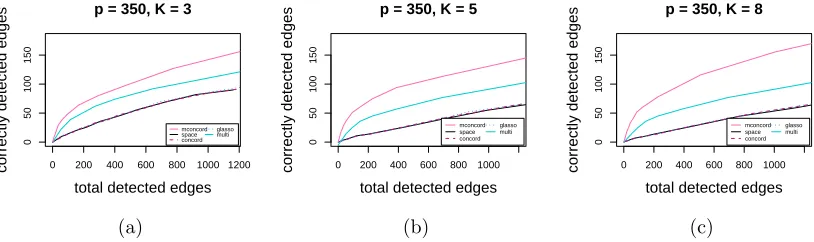
ρ is the absolute value of the smallest eigenvalue plus 0.5 and I is the identity matrix. Using each precision matrix, we generate 50 independent datasets consisting of n = 50 (for thep= 30 andp= 50 networks) andn= 100 (for the p= 100,p= 200 andp= 350 networks) i.i.d. samples. Results are given in Figure 2.1 to Figure 2.5. All figures show the number of correctly detected edges (Nc) versus the number of total detected edges

(Nt), averaged across the 50 independent datasets.

(27)

0 50 100 150 200 250

0

40

80

120

p = 30, K = 3

total detected edges

correctly detected edges

mconcord space concord glasso multi (a)

0 50 100 150 200 250

0

40

80

120

p = 30, K = 5

mconcord space concord glasso multi (b)

0 50 100 150 200 250

0

40

80

120

p = 30, K = 8

mconcord space concord glasso multi (c)

Figure 2.1: Estimation accuracy comparison: total detected edges vs. correctly detected edges with 190 true edges (44%): (a) K = 3; (b) K = 5; (c)K = 8

0 100 200 300 400

0

20

60

100

p = 50, K = 3

0 100 200 300 400

0

20

60

100

p = 50, K = 5

0 100 200 300 400

0

20

60

100

p = 50, K = 8

0 100 200 300 400 500

0

20

40

60

80

p = 100, K = 3

0 100 200 300 400 500

0

20

40

60

80

p = 100, K = 5

0 100 200 300 400 500

0

20

40

60

80

p = 100, K = 8

(28)

0 200 400 600 800

0

40

80

120

p = 200, K = 3

0 200 400 600 800

0

40

80

120

p = 200, K = 5

0 200 400 600 800

0

40

80

120

p = 200, K = 8

0 200 400 600 800 1000 1200

0

50

100

150

p = 350, K = 3

0 200 400 600 800 1000

0

50

100

150

p = 350, K = 5

0 200 400 600 800 1000

0

50

100

150

p = 350, K = 8

(29)

thatmconcordconsistently outperforms its counterparts, as it detects more correct edges than the other methods for the same number of total edges detected, especially when we have large K or large p. In all scenarios, space, concord and glasso give very similar results. For large K and p, multi performs better than univariate methods.

The better performance of moncord over space, concord and glasso is largely due to the fact thatmconcordis designed for multivariate network, and treating the precision matrix by different blocks is more likely to catch an edge even when the signal is com-parably weak. On the contrary, the univariate approaches tend to select more unwanted edges since there is high probability that there is at least one non-zero element in the block due to randomness.

In high dimensional settings, regression based methods have simpler quadratic loss function and are computationally faster and more efficient than that of penalized likeli-hood methods, which optimize with respect to the entire precision matrix at once. The running time formconcordis about one-third of that formulti. The higher numerical ac-curacy of regression based methods over penalized likelihood methods are often observed in the univariate setting, and hence is expected to continue in the multivariate setting as well.

2.4.2 Model Selection Comparison

Next in the second study, we compare the model selection performance of the above approaches. We fix K = 4, and conduct simulation studies for several combinations of

(30)

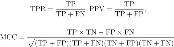
of the Bayesian Information Criterion (BIC) for model selection, but it seems that BIC does not work well in the multi-dimensional settings. In fact, BIC in most cases tends to choose the smallest model where no edge can be detected. Here we compare sensitivity (TPR), precision (PPV) and Matthew’s Correlation Coefficient (MCC) defined by

TPR = TP

TP + FN,PPV =

TP TP + FP,

MCC = _p TP×TN−FP×FN

(TP + FP)(TP + FN)(TN + FP)(TN + FN),

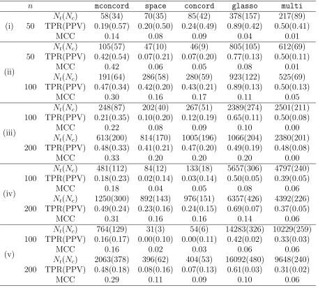
where TP, TN, FP and FN denote true positives (number of edges correctly detected), true negatives (number of edges correctly excluded), false positives (number of edges detected but absent in the true model) and false negatives (number of edges falsely ex-cluded). For each network, all final numbers are averaged across 30 independent datasets. Table 2.1 shows that substantial gain is achieved by considering the multivariate aspect inmconcordcompared with the univariate methodsspaceandconcordin regards of both sensitivity and precision, except for the casep= 30 and n= 50 where these two methods score slightly better TPR due to more selection of edges. Both glasso and

multi select very dense models in nearly all cases, and as a consequence their TPR

(31)

Table 2.1: Model selection comparison withpthe number of nodes,qthe number of true edges and n the sample size with the tuning parameter λ optimized by cross-validation. Cases considered below are (i) p= 30, q = 177 (41% density) (ii) p= 50, q= 137 (11% density), (iii) p = 100, q = 419 (8% density), (iv) p = 200, q = 617 (3% density), (v)

p= 400, q= 782 (1% density) where the density is 100q/ p₂ in percentage.

n mconcord space concord glasso multi

(i) 50

Nt(Nc) 58(34) 70(35) 85(42) 378(157) 217(89)

TPR(PPV) 0.19(0.57) 0.20(0.50) 0.24(0.49) 0.89(0.42) 0.50(0.41)

MCC 0.14 0.08 0.09 0.04 0.01

(ii) 50

Nt(Nc) 105(57) 47(10) 46(9) 805(105) 612(69)

TPR(PPV) 0.42(0.54) 0.07(0.21) 0.07(0.20) 0.77(0.13) 0.50(0.11)

MCC 0.42 0.06 0.05 0.08 0.01

100

Nt(Nc) 191(64) 286(58) 280(59) 923(122) 525(69)

TPR(PPV) 0.47(0.34) 0.42(0.20) 0.43(0.21) 0.89(0.13) 0.50(0.13)

MCC 0.30 0.16 0.17 0.11 0.05

(iii) 100

Nt(Nc) 248(87) 202(40) 267(51) 2389(274) 2501(211)

TPR(PPV) 0.21(0.35) 0.10(0.20) 0.12(0.19) 0.65(0.11) 0.50(0.08)

MCC 0.22 0.08 0.09 0.10 0.00

200

Nt(Nc) 613(200) 814(170) 1005(196) 1066(204) 2380(201)

TPR(PPV) 0.48(0.33) 0.41(0.21) 0.47(0.20) 0.49(0.19) 0.48(0.08)

MCC 0.33 0.20 0.20 0.20 0.00

(iv) 100

Nt(Nc) 481(112) 84(12) 133(18) 5657(306) 4797(240)

TPR(PPV) 0.18(0.23) 0.02(0.14) 0.03(0.14) 0.50(0.05) 0.39(0.05)

MCC 0.18 0.04 0.05 0.08 0.06

200

Nt(Nc) 1250(300) 892(143) 976(151) 6357(426) 4392(226)

TPR(PPV) 0.49(0.24) 0.23(0.16) 0.24(0.15) 0.69(0.07) 0.37(0.05)

MCC 0.31 0.16 0.16 0.14 0.06

(v) 100

Nt(Nc) 764(129) 31(3) 54(6) 14283(326) 10229(259)

TPR(PPV) 0.16(0.17) 0.00(0.10) 0.00(0.11) 0.42(0.02) 0.33(0.03)

MCC 0.16 0.02 0.03 0.06 0.06

200

Nt(Nc) 2063(378) 396(62) 404(53) 16092(480) 9648(240)

TPR(PPV) 0.48(0.18) 0.08(0.16) 0.07(0.13) 0.61(0.03) 0.31(0.02)

(32)

2.5 Application

2.5.1 Gene/Protein Network Analysis

According to the NCI website https://dtp.cancer.gov/discovery development/nci-60, “the US National Cancer Institute (NCI) 60 human tumor cell lines screening has greatly served the global cancer research community for more than 20 years. The screening method was developed in the late 1980s as an in vitro drug-discovery tool intended to supplant the use of transplantable animal tumors in anticancer drug screening. It utilizes 60 different human tumor cell lines to identify and characterize novel compounds with growth inhibition or killing of tumor cell lines, representing leukemia, melanoma and cancers of the lung, colon, brain, ovary, breast, prostate, and kidney cancers”.

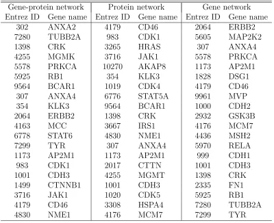
We apply our method to a dataset from the well-known NCI-60 database, which consists of protein profiles (normalized reverse-phase lysate arrays for 94 antibodies) and gene profiles (normalized RNA microarray intensities from Human Genome U95 Affymetrix chip-set for more than 17000 genes). Our analysis will be restricted to a subset of 94 genes/proteins for which both types of profiles are available. These profiles are available across the same set of 60 cancer cell lines. Each gene-protein combination is represented by its Entrez ID, which is a unique identifier common for a protein and a corresponding gene that encodes this protein.

(33)

edges are selected and for the gene network, 784 edges are selected. Protein and gene-protein networks share 313 edges, while gene and gene-gene-protein networks share 287 edges. However, protein and gene networks only share 167 edges. Table 2.2 provides summary statistics for these networks.

In Table 2.3, we also list the top 20 most connected components for all three networks. Among them, the protein network and the protein network share 11, the gene-protein network and the gene network share 10, while the gene-protein network and the gene network share only 6.

2.5.2 GDP Network Analysis

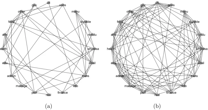
In this analysis, we apply our method to the regional GDP data obtained from U.S. De-partment of Commerce website https://www.bea.gov/index.html, which contains GDP data including the following 20 different industries with labels: (1) utilities (uti), (2) con-struction (cons) , (3) Manufacturing (manu), (4) Durable goods manufacturing (durable), (5) nondurable goods manufacturing (nondu), (6) wholesale trade (wholesale), (7) retail trade (retail), (8) transportation and warehousing (trans), (9) information (info), (10) finance and insurance (finance), (11) real estate and rental and leasing (real), (12) pro-fessional, scientific and technical services (prof), (13) management of companies and enterprises (manage), (14) administrative and waste management services (admin), (15) educational services (edu), (16) health care and social assistance (health), (17) arts, en-tertainment and recreation (arts), (18) accommodation and food services (food), (19) other services except government (other) and (20) government (gov).

(34)

im-pact of the financial crisis of that period. The data is in 8 regions in the US, including New England (Connecticut, Maine, Massachusetts, New Hampshire, Rhode Island and Ver-mont), Mideast (Delaware, D.C., Maryland, New Jersey, New York and Pennsylvania), Great Lakes (Illinois, Indiana, Michigan, Ohio and Wisconsin), Plains (Iowa, Kansas, Minnesota, Missouri, Nebraska, North Dakota and South Dakota), Souteast (Alabama, Arkansas, Florida, Georgia, Kentucky, Louisiana, Mississippi, North Carolina, South Car-olina, Tennessee, Virginia and West Virginia), Southwest (Arizona, New Mexico, Okla-homa and Texas), Rocky Mountain (Colorado, Idaho, Montana, Utah and Wyoming) and Far West (Alaska, California, Hawaii, Nevada, Oregon and Washington).

We reduce correlation in the time series data by taking differences of the consecutive observations. A multivariate network consisting of 20 nodes and 8 attributes for each node is studied. After using 5-fold cross-validation to select the tuning parameterλ, 47 edges are detected, with density of 24.7% and average node degree of 4.7. The 5 most connected industries are retail trade, transportation, wholesale trade, accommodation and food services, and professional and technical services. The network is shown in Figure 2.6(a). It is obvious to see hubs comprising of wholesale trade and retail trade. This is very natural for the consumer-driven economy of the US. Both of these two nodes are connected to transportation, as both of these industries heavily rely on transporting goods. Another noticeable fact is that education is connected with government. As part of the services provided by government, it is natural that the quality as well as GDP of educational services can both be influenced by government.

(35)

and food services, wholesale trade, professional and technical services and health care and social assistance. The network is shown in Figure 2.6(b). The more modest degree of connections in the multivariate network seems to be more interpretable.

(a) (b)

Figure 2.6: Comparison of multivariate and univariate GDP networks

2.6 Proof of Theorems

We rewrite (2.3) as L(ω, σ,Y) = 1₂Pp

i=1

PKi

k=1wik

Yik +P_j6=i

PKj

l=1ωijklY˜jl

2

, where ˜

Yik =Yik/σik.

For any subset S ⊂ T, the Karush-Kuhn-Tucker (KKT) condition characterizes a solution of the optimization problem

arg min

ω:ωSc=0

    

Ln(ω,σ, Yˆ ) +λn

X

1≤i<j≤p

v u u t

Ki

X

k=1

Kj

X

l=1 ω2

ijkl

    

(36)

A vector ˆω is a solution if and only if for any (i, j, k, l)∈S

L0_n,ijkl(ˆω,σ, Yˆ ) =−λn

ˆ

ωijkl

r P

k0_,l0

ˆ

ω2

ijk0_l0

, if ∃1≤k ≤Ki,1≤l ≤Kj,ωˆijkl 6= 0

|L0_n,ijkl(ˆω,σ, Yˆ )| ≤λn, if ˆωijkl = 0, k = 1, . . . , Ki, l= 1, . . . , Kj.

The following lemmas will be needed in the proof of Theorems 2.3.1–2.3.3. Their proofs are deferred to the Appendix.

Lemma 2.6.1 The following properties hold. (i) For all ω and σ, L(ω, σ,Y)≥0.

(ii) If σik _>₀ _{for all} ₁_≤_k _≤_K

i and i= 1, . . . , p, then L(·, σ, Y) is convex in ω and is

strictly convex with probability one.

(iii) For every index (i, j, k, l) with i6=j, L¯0_ijkl(¯ω,σ¯) = 0.

(iv) All entries of Σ¯ are bounded and bounded below. Also, there exist constants 0 <

¯

σ0 ≤σ¯∞<∞ such that

¯

σ0 ≤min{σ¯ik : 1≤i≤p,1≤k≤Ki} ≤max{σ¯ik : 1≤i≤p,1≤k ≤Ki} ≤σ¯∞.

(v) There exists constants 0<ΛL

min(¯ω,σ¯)≤ΛmaxL (¯ω,σ¯)<∞, such that

0<ΛL_min(¯ω,¯σ)≤λmin( ¯L00(¯ω,σ¯))≤λmax( ¯L00(¯ω,σ¯))≤ΛL_max(¯ω,σ¯)<∞.

(37)

def-P

j6=i Kj

P

l=1

ωijklY˜jl. Then evaluated at the true parameter values (¯ω,σ¯), we have eik(¯ω,σ¯)

un-correlated with Yjl and E(eik(¯ω,σ¯)) = 0. Since ∂L(ω, σ, Y)/∂ωijkl = wikeik(ω, σ)Yjl+

wjlejl(ω, σ)Yik, (iii) follows by taking expectation.

Since all eigenvalues of ¯Σ lie between two positive numbers, so do all diagonal entries because these are values of quadratic forms for unit vectors having 1 at one place. All off-diagonal entries lie in [−Λmax,Λmax] because these are values of bilinear forms at such

unit vectors. This shows (iv).

To prove (v), let ˜X = ( ˜X(11,21), . . . ,X(11˜ ,2K2), . . . ,X(1˜ K1,2K2), . . . ,X((˜ p−1)Kp−1,pKp)), with

˜

X(ik,jl) = (0, . . . ,0,Y˜jl,0, . . . ,0,Y˜ik,0, . . . ,0)T, a matrix of order pPp_i₌₁Ki×P_i<jKiKj,

where only the (i, k)th and (j, l)th elements are non zero. The loss function can be writ-ten as L(ω, σ, Y) = 1₂kw1/2₍_Y ₋_Xω_˜ ₎_k2

2, where w1/2 = diag(

√

w11, . . . ,

√

wpKp). Thus

¯

L00(ω, σ) = E[ ˜XT₍_w1/2₎2_X˜_{]. Let} _d ₌ P

i<jKiKj, the number of columns in ˜X, and

de-note its (i, k)th row by XT

ik, 1≤k ≤Ki, 1≤i≤p. Then for any unit vector a∈Rd, we

have

aTL¯00(¯ω,σ¯)a= E(aTX˜T(w1/2)2Xa˜ ) = E p X i=1 Ki X k=1

wik(XikTa)

2

.

Index the elements of aas (a(11,21), . . . , a(11,2K2), . . . , a(1K1,2K2), . . . , a((p−1)Kp−1,pKp))

T_{, and}

for each 1≤i≤p and 1≤k ≤Ki, define aik ∈RKip by

aik =

              

(0, . . . ,0, a(1k,21), . . . , a(1k,2K2), . . . , a(1k,p1), . . . , a(1k,pKp))

T_, _i_{= 1}_,

(a(pk,11), . . . , a(pk,1K1), . . . , a(pk,(p−1)1), . . . , a(pk,(p−1)Kp−1),0, . . . ,0)

T_, _i₌_p,

(a(11,ik), . . . , a((i−1)Ki−1,ik),0, . . . ,0, a(ik,(i+1)1), . . . , a(ik,pKp))

T_, ₁_{< i < p,}

with exactly Ki zeros and

P

j=6 iKj non-zeros. Then by definition XikTa = ˜YTaik. Also

note that p P i=1 Ki P k=1

(38)

twice in a. Therefore, since ¯L00(¯ω,σ¯) = E ˜YY˜T_{, we have}

aTL¯00(¯ω,σ¯)a=

p

X

i=1

Ki

X

k=1

wikaTikΣ˜aik≥ p

X

i=1

Ki

X

k=1

wikλmin( ˜Σ)kaikk22 ≥2w0λmin( ˜Σ),

where ˜Σ = var( ˜Y). Similarly, aT_L_¯00_(¯_ω₎_a _≤ ₂_w

∞λmax( ˜Σ). By Condition (C1), ˜Σ has

bounded eigenvalues, and hence (v) follows.

Lemma 2.6.2 (i) There exists a constant N < ∞, such that for all 1 ≤ i 6= j ≤ p

and 1≤k≤Ki, 1≤l≤Kj, L¯00ijkl,ijkl(¯ω,σ¯)≤N.

(ii) There exists constants M1, M2 <∞, such that for any 1≤i < j ≤p,

Var(L0_ijkl(¯ω,σ, Y¯ ))≤M1, Var(L00ijkl,ijkl(¯ω,σ, Y¯ ))≤M2.

(iii) There exists a positive constant g, such that for all (i, j, k, l)∈ A,

L00_ijkl,ijkl(¯ω,σ¯)−L00_ijkl,_A₋

ijkl(¯ω,σ¯)

h

L00_A₋

ijkl,A−ijkl(¯ω,σ¯)

i−1 L00_A

ijkl,ijkl(¯ω,σ¯)≥g,

where A−ijkl=A \ {(i, j, k, l)}.

(iv) For any (i, j, k, l) ∈ Ac_, _k_L_¯00

ijkl,A(¯ω,σ¯)[ ¯L00A,A(¯ω,σ¯)]−1k2 ≤ M3. for some constant M3.

Proof 2 (of Lemma 2.6.2) The proof of (i) follows because ¯L00_ijkl,i0_j0_k0_l0(¯ω,σ¯) = σ_jl,j0_l0+

(39)

For (ii) note that Var(eik(¯ω,σ¯)) = 1/σ¯ik and Var(Yik) = ¯σik,ik,

Var(L0_n,ijkl(¯ω,σ, Y¯ )) = Var(wikeik(¯ω,σ¯)Yjl) + Var(wjlejl(¯ω,σ¯)Yik)

≤E(w2_ike2_ik(¯ω,σ¯)Y_jl2) + E(w2_jle2_jl(¯ω,σ¯)Y_ik2) = w

2

ik¯σjl,jl

¯

σik +

w2

jl¯σik,ik

¯

σjl .

The right hand side is bounded because of Condition (C0) and Lemma 2.6.1(iv), and the fact that eik(¯ω,σ¯) and Yjl are independent.

For (i, j, k, l)∈ A, denote

D:= ¯L00_ijkl,ijkl(¯ω,σ¯)−L¯00_ijkl,_A₋

ijkl(¯ω,σ¯)

h ¯

L00_A₋

ijkl,A−ijkl(¯ω,σ¯)

i−1 ¯

L00_A₋

ijkl,ijkl(¯ω,σ¯).

Then D−1 _{is the (}_{ijkl, ijkl}_{)th entry in} h_L_¯00

A,A(¯ω,σ¯) i−1

. Thus by Lemma 2.6.1(v),D−1 _is

positive and bounded from above, soD is bounded away from zero. This proves (iii). Note thatkL¯00_ijkl,_A(¯ω,σ¯)[ ¯L00_A_,_A(¯ω,σ¯)]−1_k2

2 ≤ kL¯

00

ijkl,A(¯ω,σ¯)k22λmax([ ¯L00A,A(¯ω,σ¯)]−2).

By Lemma 2.6.1(iv), λmax([ ¯L00A,A(¯ω,σ¯)]−2) is bounded from above, thus it suffices to show that kL¯00_ijkl,_A(¯ω,σ¯)k2

2 is bounded. DefineA+ := (i, j, k, l)∪ A. Then ¯L00ijkl,ijkl(¯ω,σ¯)−

¯

L00_ijkl,_A(¯ω,σ¯)[ ¯L00_A_,_A(¯ω,σ¯)]−1L¯00_A_,ijkl(¯ω,σ¯) is the inverse of the (kl, kl) entry of ¯L00_A+_,_A+(¯ω,σ¯).

Thus by Lemma 2.6.1(iv), it is bounded away from zero. Therefore by Lemma 2.6.2(i), ¯

L00_ijkl,_A(¯ω,σ¯)[ ¯L00_A_,_A(¯ω,σ¯)]−1_L_¯00

A,ijk(¯ω,σ¯) is bounded from above. Since

¯

L00_ijkl,_A(¯ω,σ¯)[ ¯L00_A_,_A(¯ω,σ¯)]−1L¯00_A_,ijk(¯ω,σ¯)≥ kL¯00_ijkl,_A(¯ω,σ¯)k2

2λmin([ ¯L00A,A(¯ω,σ¯)] −1₎_,

and by Lemma 2.6.1(iv), λmin([ ¯L00A,A(¯ω,¯σ)]−1) is bounded away from zero, we have

kL¯00_ijkl,_A(¯ω,σ¯)k2

2 bounded from above. Thus (iv) follows.

(40)

1≤k≤Ki, 1≤l≤Kj, kE[YikYjlY˜Y˜T]k ≤M4.

Proof 3 (of Lemma 2.6.3) The (i0k0, j0l0)th entry of the matrixYikYjlY˜Y˜T is

YikYjlY˜i0_k0Y˜_j0_l0, for 1≤i < j ≤p, 1≤ k0 ≤K_i0 and 1≤l0 ≤ K_j0. Hence, the (i0k0, j0, l0)th

entry of the matrix E[YikYjlY˜Y˜T] is

E[YikYjlY˜i0_k0Y˜_j0_l0] = (¯σ_ik,jlσ¯_i0_k0_,j0_l0 + ¯σ_ik,i0_k0σ¯_jl,j0_l0 + ¯σ_ik,j0_l0σ¯_jl,i0_k0)/(¯σi 0_k0

¯

σj0l0),

where ¯σik,jl denotes the covariance betweenYik and Yjl. Thus, we can write

E[YikYjlY˜Y˜T] =

1 ¯

σi0_k0

¯

σj0_l0(¯σik,jlΣ + ¯¯ σik,·¯σ

T

jl,·+ ¯σjl,·¯σik,T ·), (2.7)

where ¯σik,·is the Pp_j₌₁Kj vector (¯σik,jl :l= 1, . . . , Kj, j = 1, . . . , p, j 6=i). Then we have

kE[YikYjlY˜Y˜T]k ≤

1

|σ¯i0_k0

¯

σj0_l0

|(|¯σik,jl|kΣ¯k+ 2kσ¯ik,·k2kσ¯jl,·k2), (2.8)

where k·k is the operator norm. By Condition (C1), |σ¯i0k0σ¯j0l0|−1 _and _|_σ_¯

ik,jl|kΣ¯k are

uni-formly bounded. Further ¯σik,ik−σ¯ik,T ·Σ¯ −1

(−ik)σ¯ik,· > 0, where ¯Σ(−ik) is the submatrix of ¯Σ

removing ikth row and column. From this, it follows that

kσ¯ik,·k2 =kΣ¯

1/2

−(ik)Σ¯

−1/2

−(ik)σ¯ik,·k2 ≤ kΣ¯ 1/2

−(ik)kkΣ¯

−1/2

−(ik)σ¯ik,·k ≤

q

kΣ¯kp

¯

σik,ik, (2.9)

which follows from the fact that ¯Σ(−ik) is a principal submatrix of ¯Σ.

Lemma 2.6.4 Let the conditions of Theorem 2.3.2 hold. Then for any sequence Cn →

∞,

max

_L0 _(¯_ω,_σ,_¯ _Y₎₋_L0 _(¯_ω,_σ,_ˆ _Y₎ _≤_C

n

r logn

(41)

max i<j,t<s L 00

n,ijkl,tsk0_l0(¯ω,σ,¯ Y)−L00_n,ijkl,tsk0_l0(¯ω,σ,ˆ Y)

≤Cn

r logn

n ,

hold with probability tending to 1.

Proof 4 (of Lemma 2.6.4) Observe thatL0_n,ijkl(¯ω, σ,Y) is given by

1 n n X m=1 wik

Y_ikm+X

j0₆₌_i

K_j0

X

l0₌₁

ωij0_k0_l0

σik Y m j0_l0

_Ym jl

σik +wjl

Y_jlm+X

i0₆₌_j

Ki0

X

k0₌₁

ωij0_k0_l0

σjl Y m i0_k0

Y_ikm σjl.

ThusL0_n,ijkl(¯ω,σ,¯ Y)−L0_n,ijkl(¯ω,σ,ˆ Y) is given by

wik

YikYjl(

1 ¯

σik −

1 ˆ

σik) +

X

j0₆₌_i

K_j0

X

l0₌₁

Yj0_l0Y_jl(

1 (¯σik₎2 −

1 (ˆσik₎2)

+wjl

YikYjl(

1 ¯

σjl −

1 ˆ

σjl) +

X

i0₆₌_j

Ki0

X

k0₌₁

Yi0_k0Y_ik(

1 (¯σjl₎2 −

1 (ˆσjl₎2)

,

whereYikYjl= _n1 n

P

m=1 Ym

ikYjlm. By Lemma 2.6.1(iv),{σ¯ik,jl : 1≤i, j ≤p,1≤k, l≤K} are

bounded from below and above, and hence maxi,j,k,l|YikYjl−σ¯ik,jl| = Op(

p

(logn)/n). This implies that maxi,j,k,l|YikYjl|=Op(1), and hence by Lemma 2.6.1(iv) and Condition

(C3) it follows that

max

i,j,k,l|L

0

n,ijkl(¯ω,σ,¯ Y)−L

0

n,ijk(¯ω,σ,ˆ Y)|=Op

r logn

n

!

.

The bound for |L00_n,ijkl,tsk0_l0(¯ω,σ,¯ Y)−L00_n,ijkl,tsk0_l0(¯ω,σ,ˆ Y)| follows similarly.

Lemma 2.6.5 Let Xij i.i.d.

∼ N(0, σ2

xi) and Yij i.i.d.

∼ N(0, σ2

yi) for i = 1, . . . , m and j =

1, . . . , n, andXij andYij are independent for alli. Further assume that0< σxi, σyi ≤σ <

∞. Then for any sequenceCn→ ∞, we havemax1≤i≤m|n−1

Pn

j=1XijYij| ≤Cn

p

(42)

Proof 5 (of Lemma 2.6.5) For fixed i we can observe that

E|n−1Xi1Yi1|r =

1

nrE|Xi1| r_E_|_Y

i1|r ≤

2r_σr

nr

(Γ(r+1₂ ))2

π ≤(2σ/n)

r−24σ2 πn2r!.

By Lemma 2.2.11 of Van Der Vaart & Wellner [38], takingM = 2σ/nandv = 8σ2/πn, we have P|n−1Pn

j=1XijYij| > x

≤ 2e−x2_/_[2(8_σ2_/πn₊₂_σx/n_)]

. Then by Lemma 2.2.10 of Van Der Vaart & Wellner [38], for some C >0, Emax

1≤i≤m|n

−1Pn

j=1XijYij|

≤Cp(logm)/n,

which implies the conclusion.

Lemma 2.6.6 If K2

maxqn = o(

p

n/logn), then for any sequence Cn → ∞ and any u ∈

R|A|, the following hold with probability tending to 1:

kL0_n,_A(¯ω,σ,ˆ Y)k2 ≤ CnKmax

r

qnlogn

n ,

|uTL0_n,A(¯ω,σ,ˆ Y)| ≤ Cnkuk2Kmax

r

qnlogn

n ,

|uTL00_n,_A_,_A(¯ω,σ,ˆ Y)u−uTL¯00_A_,_A(¯ω,σ¯)u| ≤ Cnkuk22K

2 maxqn

r logn

n ,

kL00_n,_A_,_A(¯ω,σ,ˆ Y)u−L¯00_A_,_A(¯ω,σ¯)uk2 ≤ Cnkuk2Kmax2 qn

r logn

n .

Proof 6 (of Lemma 2.6.6) If we replace ˆσby ¯σon the left hand side and take (i, j, k, l)∈ A, then from the definition we have L0_n,ijkl(¯ω,σ,¯ Y) = eik(¯ω,σ¯)TYjl + ejl(¯ω,σ¯)TYik,

and Yjl, where eik are n replications of eik( ¯ω,¯σ). Thus by Lemma 2.6.5 we obtain

max{|L0_n,ijkl(¯ω,σ,ˆ Y)| : (i, j, k, l)∈ A} ≤ Cn

p

(logn)/n. and hence by the Cauchy-Schwartz inequality

kL0_n,A(¯ω,σ,ˆ Y)k2 ≤Kmax

√

qn max

(i,j,k,l)∈A|L 0

n,ijkl(¯ω,σ,ˆ Y)| ≤CnKmax

r

qnlogn

(43)

andkL0_n,_A(¯ω,σ,ˆ Y)k2 ≤ kL0n,A(¯ω,σ,¯ Y)k2+kL0n,A(¯ω,σ,¯ Y)−L0n,A(¯ω,σ,ˆ Y)k2. The second

term on the right hand side has order Kmax

p

qn(logn)/n. Since there are Kmax2 qn terms

and by Lemma 2.6.4, they are uniformly bounded byp(logn)/n. The rest of the lemma can be proved by similar arguments.

Lemma 2.6.7 Assume that the conditions of Theorem 2.3.1 hold. Then exists a constant

¯

C1 > 0, such that with probability tending to 1, there exists a local minimum of the

restricted problem (2.6) within the disc {ω :kω−ω¯k2 ≤C¯1Kmax

√

qnλn}.

Proof 7 (of Lemma 2.6.7) Let αn = Kmax

√

qnλn, and Ln(ω,σ,ˆ Y) = Ln(ω,σ,ˆ Y) +

λP P

i<jkωijk2. Then for any given constant ¯C1 >0 and any vector usuch thatuAc = 0

and kuk2 = ¯C1, the triangle inequality and the Cauchy-Schwartz inequality together

imply that

X

i<j

kω¯ijk2−

X

i<j

kω¯ij +αnuijk2 ≤αn

p

K2

maxqnkuk2 = ¯C1αnKmax

√

qn.

ThusLn(¯ω+αnu,σ,ˆ Y, λn)− Ln(¯ω,σ,ˆ Y, λn) can be written as

{Ln(¯ω+αnu,ˆσ,Y)−Ln(¯ω,σ,ˆ Y)} −λn{

X

i<j

kω¯ijk2−

X

i<j

kω¯ij +αnuijk2}

≥ {Ln(¯ω+αnu,σ,ˆ Y)−Ln(¯ω,σ,ˆ Y)} −C¯1αnKmax

√

qnλn

(44)

Thus for any sequence Cn→ ∞, with probability tending to 1,

Ln(¯ω+αnu,σ,ˆ Y)−Ln(¯ω,σ,ˆ Y)

=αnuTAL 0

n,A(¯ω,σ,ˆ Y) + 1 2α 2 nu T AL 00

n,A,A(¯ω,σ,ˆ Y)uA =1

2α

2

nu T

AL¯ 00

n,A,A(¯ω,σ¯)uA+ 1 2α 2 nu T A

L_n,00_A_,_A(¯ω,σ,ˆ Y)−L¯00_n,_A_,_A(¯ω,σ¯)uA+αnuTAL 0

n,A(¯ω,σ,ˆ Y)

≥1

2α

2

nu T

AL¯ 00

n,A,A(¯ω,σ¯)uA−Cnα2nK

2

maxqnn−1/2

p

logn−CnαnKmaxqn1/2n

−1/2p logn.

In the above, the first equation holds because the loss functionL(ω, σ, Y) is quadratic in

ω and uAc = 0. The inequality is due to Lemma 2.6.6.

By the assumptions that K2

maxqn = o(

p

n/logn) and λn

p

n/logn → ∞, we have

α2

nKmax2 qnn−1/2

√

logn=o(α2

n) and αnKmaxq 1/2

n n−1/2

√

logn=o(α2

n). Thus,

Ln(¯ω+αnu,σ,ˆ Y, λn)− Ln(¯ω,σ,ˆ Y, λn)≥

1 4α

2

nuTAL¯ 00

A,A(¯ω,σ¯)uA−C¯1α2n

with probability tending to 1. By Lemma 2.6.1 (iv), uT

AL¯00A,AuA ≥ ΛminL (¯ω,σ¯)kuAk22 =

ΛL

min(¯ω,σ¯) ¯C12, thus if we take ¯C1 = 5/ΛLmin(¯ω,σ¯), then

Pinf{Ln(¯ω+αnu,σ,ˆ Y, λn) :u:uAc = 0,kuk₂ = ¯C₁}>L_n(¯ω,σ,ˆ Y, λ_n) →1.

Hence a local minimum exists in{ω :kω−ωˆk2 ≤C¯1Kmax

√

qnλn}with probability tending

to 1.

Lemma 2.6.8 Assume the conditions of Theorem 2.3.1. Then exists a constant C2¯ >

0 such that for any ω satisfying kω − ω¯k2 ≥ C¯2Kmax

√

qnλn and ωAc = 0, we have

kL0_n,_A(ω,σ,ˆ Y)k2 > Kmax

√

qnλn with probability tending to 1.

(45)

lemma can be written asω = ¯ω+αnu, with uAc = 0 andkuk₂ ≥C¯₂, where ¯C₂ >0. Note

that

L0_n,_A(ω,σ,ˆ Y) = L0_n,_A(¯ω,σ,ˆ Y) +αnL00n,A,A(¯ω,σ,ˆ Y)u =L0_n,_A(¯ω,σ,ˆ Y) +αn

L00_n,_A_,_A(¯ω,σ,ˆ Y)−L¯00_A_,_A(¯ω,σ¯)u+αnL¯00A,A(¯ω,σ¯)u.

By the triangle inequality and Lemma 2.6.6, for any Cn → ∞, kL0n,A(ω,σ,ˆ Y)k2 is

bounded below by

αnkL¯00A,A(¯ω,σ¯)uk2−Cn(Kmaxqn1/2n

−1/2p

logn)−Cnkuk2(αnKmax2 qnn−1/2

p logn)

with probability tending to 1. Thus, as argued in the proof of Lemma 2.6.7,

αnKmaxq1n/2n−1/2

√

logn=o(αn) and αnKmax2 qnn−1/2

√

logn=o(αn), then

kL0_n,_A(ω,σ,ˆ Y)k2 ≥ 1₂αnkL¯00A,A(¯ω,σ¯)uk2with probability tending to 1. By Lemma 2.6.1(iv),

kL¯00_A_,_A(¯ω,σ¯)uk2 ≥ΛLmin(¯ω,¯σ)kuk2. Therefore ¯C2 can be taken as 3/ΛLmin(¯ω,σ¯).

Lemma 2.6.9 LetDA,A(¯ω,σ, Y¯ ) = L00A,A(ω,σ, Y¯ )−L¯00A,A(¯ω,σ¯). Then there exists a

con-stant M5 <∞, such that for any (i, j, k, l)∈ A, λmax(Var(DA,ijkl(¯ω,σ, Y¯ )))≤M5.

Proof 9 (of Lemma 2.6.9) Observe that

Var(DA,ijkl(¯ω,σ, Y¯ )) = E(L00A,ijkl(¯ω,σ, Y¯ )L

00

A,ijkl(¯ω,σ, Y¯ ) T

)−L¯00_A_,ijkl(¯ω,σ¯) ¯L00_A_,ijkl(¯ω,σ¯)T.

Thus it suffices to show that there exists a constant M5 >0, such that for all (i, j, k, l), λmax(E(L00A,ijkl(¯ω,σ, Y¯ )L

00

A,ijkl(¯ω,σ, Y¯ )T)) ≤ M5. We use the same notations as in the

proof of Lemma 2.6.1(v).

(46)

E(L00_A_,ijkl(¯ω,σ, Y¯ )L00_A_,ijkl(¯ω,¯σ, Y)T_{) is given by}

E[Y_ik2XjlXjlT] + E[Y

2

jlXikXikT] + E[YikYjl(XjlXjlT +XikXikT)],

and for a∈_Rd_,

aTEω,¯¯σ(L00A,ijkl(¯ω,σ, Y¯ )L

00

A,ijkl(¯ω,¯σ, Y) T_a

=aT_jlE[Y_ik2Y˜Y˜T]ajl+aTikE[Y

2

jlY˜Y˜ T_]_a

ik+ 2aTikE[YikYjlY˜Y˜T]ajl.

Since Pp

i=1

PKi

k=1kaikk22 = 2kak22 = 2,and by Lemma 2.6.3 λmax(E[YikYjlY˜Y˜T])≤ M4 for

any 1≤i < j ≤pand 1≤k ≤Ki, 1≤l ≤Kj, the conclusion follows.

Proof 10 (of Theorem 2.3.1) The existence of a solution of (2.6) follows from Lemma 2.6.7. By the KKT condition, any solution ˆω of (2.6), satisfies

kL0_n,_A(ˆω,σ,ˆ Y)k∞ ≤λn, implying

kL0_n,_A(ˆω,σ,ˆ Y)k2 ≤ Kmax

√

qnkL0n,A(ˆω,σ,ˆ Y)k∞ ≤ Kmax

√

qnλn. Thus by Lemma 2.6.8,

with probability tending to 1, all solutions of (2.6) are inside the disc {ω : kω−ω¯k2 ≤

¯

C2Kmax

√

qnλn}. Hence with probability tending to 1, kωˆλAn−ω¯Ak2 ≤C¯2(¯ω)Kmax

√

qnλn.

Proof 11 (of Theorem 2.3.2) By the KKT condition and the expansion of

L0_n,_A(ˆωλn

A ,σ,ˆ Y) at ¯ω,

−λnMˆA =L0n,A(ˆωAλn,σ,ˆ Y) =L

0

n,A(¯ω,ˆσ,Y) +L 00

n,A,A(¯ω,σ,ˆ Y)νn

= ¯L00_A_,_A(¯ω,σ¯)νn+L0n,A(¯ω,σ,ˆ Y) + h

(47)

where νn := ˆωAλn −ω¯A and ˆMA = (ˆωijkl/

r P

k0_,l0

ˆ

ω2

ijk0_l0 : (i, j, k, l)∈ A)T. Therefore

νn=−λn[ ¯L00A,A(¯ω,σ¯)]

−1_M_ˆA₋

[ ¯L00_A_,_A(¯ω,σ¯)]−1hL0_n,_A(¯ω,σ,ˆ Y) +Dn,A,A(¯ω,σ,ˆ Y)νn

i

, (2.10)

where Dn,A,A(¯ω,σ,ˆ Y) = L00n,A,A(¯ω,σ,ˆ Y) −L¯00A,A(¯ω,σ¯). Next, fix (i, j, k, l) ∈ Ac, and consider the expansion of L0_n,ijk(ˆωλn

A ,σ,ˆ Y) around ¯ω is given by

L0_n,ijkl(¯ω,σ,ˆ Y) +L00_n,ijkl,A(¯ω,σ,ˆ Y)νn

=L0_n,ijkl(¯ω,σ,ˆ Y) + ¯L00_ijkl,_A(¯ω,σ¯)νn+

h

L00_n,ijkl,_A(¯ω,σ,ˆ Y)−L¯00_ijkl,_A(¯ω,σ¯)iνn

=L0_n,ijkl(¯ω,σ,ˆ Y) + ¯L00_ijkl,_A(¯ω,σ¯)νn+Dn,ijkl,A(¯ω,σ,ˆ Y)νn. (2.11)

Then plugging (2.10) into (2.11) and rearranging, L0_n,ijkl(ˆωλn

A ,σ,ˆ Y) is given by

L0_n,ijkl(¯ω,σ,ˆ Y)−λnL¯00ijkl,A(¯ω,σ¯)[ ¯L 00

A,A(¯ω,σ¯)] −1_M_ˆA

−L¯00_ijkl,_A(¯ω,σ¯)[ ¯L00_A_,_A(¯ω,σ¯)]−1L0_n,_A(¯ω,σ,ˆ Y) +

h

Dn,ijkl,A(¯ω,σ,ˆ Y)−L¯00ijkl,A(¯ω,σ¯)[ ¯L00A,A(¯ω,σ¯)]−1Dn,A,A(¯ω,σ,ˆ Y)

i

νn. (2.12)

By Condition (C2), for any (i, j, k, l)∈ Ac _: _|_L_¯00

ijkl,A(¯ω,σ¯)[ ¯L00A,A(¯ω,σ¯)]−1M| ≤ δ < 1. By Theorem 2.3.1, we have kωˆλn

A −ω¯Ak2 = Op(Kmax

√

qnλn) = op(1), then |MˆA −M| =

op(1). Hence for any (i, j, k, l) ∈ Ac : |L¯00ijkl,A(¯ω,¯σ)[ ¯L00A,A(¯ω,σ¯)]−1MˆA| ≤ δ < 1. Thus it suffices to prove that the remaining term in (2.12) are o(λn) with probability tending

to 1 uniformly for all (i, j, k, l) ∈ Ac_{. Then since} _|Ac_{| ≤} _K2

maxp2 = O(n2κ), the event

max(i,j,k,l)∈Ac|L0_n,ijkl(ˆω_Aλn,σ,ˆ Y)|< λ_n happens with probability tending to 1.

By Lemma 2.6.2(iv), for any (i, j, k, l) ∈ Ac_, _k_L_¯00