Evolutionarily stable mutation rate in a periodically changing environment.

(1)

Copyright 0 1989 by the Genetics Society of America

Evolutionarily Stable Mutation Rate

in a

Periodically Changing Environment

**Kazushige Ishii,* Hirotsugu Matsuda: Yoh Iwasat and Akira Sasakit**

*College of General Education, Nagoya University, Nagoya 464, Japan and tDepartment of Biology, Faculty ofscience, Kyushu University, Fukuoka 812, Japan

Manuscript received December 9, 1987 Accepted for publication September 23, 1988

ABSTRACT

Evolution of mutation rate controlled by a neutral modifier is studied for a locus with two alleles under temporally fluctuating selection pressure. A general formula is derived to calculate the evolutionarily stable mutation rate in an infinitely large haploid population, and following results are obtained. (I) For any fluctuation, periodic or random: (1) if the recombination rate r per generation between the modifier and the main locus is 0, pa is the same as the optimal mutation rate pop which maximizes the long-term geometric average of population fitness; and (2) for any r , if the strength s of selection per generation is very large, bm is equal to the reciprocal of the average number T of

generations (duration time) during which one allele is persistently favored than the other. (11) For a periodic fluctuation in the limit of small s and r , p e s s ~ is a function of ST and rT with properties: (1) for

a given ST, perr7 decreases with increasing rT; (2) for ST d 1, P-T is almost independent of S T , and

depends on rT as p c L e u ~

=

1.6 for rT << 1 and p e m ~ k 6 / r ~ for rT >> 1 ; and (3) for ST

B

1, and for a given

r r , p e s r ~ decreases with increasing ST to a certain minimum less than 1, and then increases to 1

asymptotically in the limit of large ST. (HI) For a fluctuation consisting of multiple Fourier components @ e . , sine wave components), the component with the longest period is the most effective in determining pes (low passjlter effect). (IV) When the cost c of preventing mutation is positive, the modifier is non- neutral, and pes becomes larger than in the case of neutral modifier under the same selection pressure acting at the main locus. The value of c which makes equal to clop of the neutral modifier case is

calculated. It is argued that this value gives a critical cost such that, so long as the actual cost exceeds this value, the evolution rate at the main locus must be smaller than its mutation rate pes.

I

N a constant environment, mutation is deleterious since it brings about a mutational load to the population by producing unfit alleles from a common one which is often best fit to the environment. Theo- retical studies of mutation rate modifier dynamics conclude that the rate should evolve toward zero (for example, LIEBERMAN and FELDMAN 1986). In a fluctuating environment, however, the rate can evolve toward a nonzero level since mutation is advantageous as long as it provides genetic variation necessary for a population to adapt to the changing environment.

This idea was put forward by STURTEVANT (1 937), and was quantitatively studied by KIMURA (1960,

1967). KIMURA proposed that mutation rate would evolve toward a rate which minimizes the sum of the mutation load L , and the substitution load Le. LEVINS (1967) further developed this idea by calculating the optimal mutation rate pop which maximizes the long- term geometric average of population fitness for a model that explicitly incorporated a fluctuating environment. Recently, ISHII and MATSUDA (1 985) proved that the optimal mutation rate pop is equal to the evolution rate v which is defined as the rate of mutant substitutions that have occurred along the phylogenic line leading to the present organisms.

Genetics 121: 163-174 (January, 1989)

However, all of these papers implicitly assumed that the mutation rate is adjusted through group selection. So, their conclusions need to be compared with those of modifier theories in which the mutation rate evolves through individual selection. This is because a population which is best fit with respect to group selection can sometimes be unstable against the invasion of a mutant modifier through individual selection.

LEIGH (1970, 1973) studied for the first time a

mutation modifier model in fluctuating environment. For a special case of very strong selection, he showed that a nonzero optimal level is realized by neutral modifiers in a n asexual population. He further argued that in a sexual population selection would adjust the mutation rate toward zero, but did not explicitly calculate the level of mutation rate attained by modifiers.

GILLESPIE (1981) studied a modifier model similar to

LEIGH’S but in a rapidly fluctuating environment

(2)

164 et al.

mediate rate. This result is qualitatively different from

LEIGH’S.

In this paper we study a population genetic model of mutation rate modifiers in an infinitely large haploid population. We derive a formula by which we can calculate the evolutionarily stable mutation rate pess

which is to be realized as an evolutionary consequence. We examine how pess depends on the strength and duration of periodically fluctuating selection and the recombination between the modifier and the main locus. We find that selection would generally adjust

pess at a nonzero level even in the weak selection limit or by unlinked modifiers. We discuss possible differences of peSs between a periodic environment and a random one. Finally, we calculate the effect of non- neutral modifiers for a case of positive cost of preventing mutation, and discuss its implication on the molecular evolution rate at the main locus.

MODIFIER MODEL

We consider a two-locus model of mutation rate modifiers in a haploid population of effectively infinitely large size. T h e main locus with two alleles A

and a is under a fluctuating selection such that the relative fitnesses of A and a in the tth generation are

1

+

s(t) and 1

-

s(t), respectively. T h e selection coefficient s(t) fluctuates through time with the average 0 .

The modifier locus with two alleles B and b controls the mutation rate between A and a at the main locus as p and p’ for B and b, respectively. T h e recombination rate between the modifier and the main locus is

r per generation. T h e modifier alleles are selectively neutral so that the fitness of a genome does not depend on them.

Consider a population which is made up of only B-

carrying genomes. We introduce a small fraction of mutant modifier b carrying genomes with a different mutation rate p’ into it, and ask if the mutant modifier increases in the population or not. If no mutant modifier b in a given set of modifiers can increase in the population, the resident modifier B is said to be evolutionarily stable (MAYNARD SMITH and PRICE 1973), and we call the mutation rate p caused by B an evolutionarily stable mutation rate peSs. As a consequence of repeated introduction of new modifiers, we expect that the mutation rate would evolve toward

P C S S .

We can analyze the elimination of an introduced b

modifier by a following linear dynamical system model since b carrying genomes can be assumed to remain rare in the population throughout the course. let N l ( t )

and N 2 ( t ) be, respectively, the numbers of A b carrying genomes and ab carrying ones in the population at time t. Then, the corresponding numbers at the next

time t

+

1 are obtained in three steps as follows. First, genic selection amplifies them as

N ; = (1

+

s(t))N&),

N4

= (1

-

s(t))Np(t).

Next, mutation with rate p’ modifies them as

N;‘

= (1

-

p’)Nl

+

p ‘ N 4 ,

N;

= p ’ N i

+

(1

-

p ’ ) N 4 .

Finally, recombination completes the change in one generation as

Nl(t

+

1) = {(l

-

r )

+

rx1(t))N;’

+

rxl(t)N;,

NB(t

+

1) = rx2(t)N;’

+

((1

-

r )

+

rxp(t))N!.

Here, xl(t) and ~ ( t ) are, respectively, the frequencies

of A and a among B carrying genomes just before

recombination takes place. Recombination with b carrying genomes is neglected since they are rare in the population.

Combining above three steps, we obtain the numbers of b carrying genomes at time t

+

1 from those at time t as

where 2 X 2 matrix M ( t ) is given by

M ( t ) =

I“

-

r x z ( t )

-

(1

-

r)p’l{l

+

s(t)) b x e ( t )

+

(1

-

+’){1

+

s(t))

1

(2) h ( t )

+

(1

-

r)p’l{l

-

s(t)l

{ 1

-

rx$)

-

(1

-

r ) p ’ ) ( 1

-

s ( t ) )

.

In order to apply (1) and (2) to study the ultimate fate of b carrying genomes, we must first know values of frequencies x l ( t ) and ~ ( t ) = 1

-

x l ( t ) of A and a

among B carrying genomes at each time t. When the population consists of only B genomes, their time change is due to fluctuating selection and mutation with rate p, and is given by

This applies also after the introduction of b carrying genomes as long as they remain rare in the population, because recombination with them can be neglected.

According to ( l ) , the long-term increase rate

X = Iim { N ( ~ ) / N ( o ) ) ” ~

of the total number N ( t ) = N l ( t )

+

NZ(t) of b carrying genomes is determined by the multiplication of matrices {M(t); t = 0 , l , 2,

. .

.).

Since the matrix M ( t )

in (2) depends not only on p‘ but also on p through

x i ( t ) determined by (3), the rate X is a function of both p’ and p, say X ( p ’ , p). Then, in order that p be stable

(3)

-Evolutionarily Stable Mutation Rate 165

against the introduction of modifier alleles with a slightly different p’, X(p’, p) must be smaller than X(p, p). This gives

A(p) = [ W p ’ , p)/d~’l~,=~ = 0 ( 4 4

together with

A@’) P 0 for p P p’ (4b)

as the condition for p to be an evolutionarily stable mutation rate pess.

T h e long-term increase rate X is equal to the long- term geometric average lim{G(t

-

I)G(t

-

2)

.

*

.

t “ t m

G(O)}l’I of

G(t) = [{l

+

S(t)Wl(t)

+

(1

-

S(t)IN2(t)l/N(t)

since N ( t ) = G(t

-

l)G(t

-

2)

-

.

zZ(O)N(O) according to (1)-(2). Here, G(t) is the average fitness of a subpopulation of b carrying genomes. It is a function of not only p’ but also p as long as M ( t ) in (2) depends on p. In a particular case where the modifier locus is completely linked with the main locus ( r = 0 ) , M ( t )

does not depend on p , hence X is independent of p and is equal to the long-term geometric average of population fitness for the case of a homogeneous modifier locus with mutation rate

i’.

Therefore we can conclude by (4) that f o r completely linked modijiers, pes, is the same as the optimal mutation rate pop which maximizes the long-term geometric average of population fitness.

However, in general cases, some recombination may occur each generation between the modifier and the main locus ( r

>

0). Then the optimal mutation rate

pop may not be attained as a consequence of natural selection. In order to study more clearly what happens in this case, we concentrate in the following on the periodically fluctuating environment with a finite period T. Possible differences in results between a periodic environment and a random one will be dis- cussed later.

In a periodic environment with period T , the selection coefficient s(t) is a periodic sequence with period T. Then, since the periodic transformation (3) with period T has been exerted for a long time, time

sequences of x l ( t ) and xp(t) must have converged to periodic ones with the same period T by the time of introduction of b carrying genomes,’ and remain

so as long as b carrying genomes are rare in the population. T h e periodic sequence of x l ( t ) is obtained by solving simultaneous equations (3) for t = 0, 1,

2 , . ” , T

-

1 under a boundary condition x l ( T ) =

XI(0).

Since we now know that time sequences of x l ( t ) and

’ The convergence to periodic sequences with period T can be proved by noting that apparently nonlinear transformation (3) of the frequency xl(t) is but with r = 0 and p’ replaced by p.

related to a periodic linear transformation of genome numbers like (1)-(2)

x2(t) are periodic with period T, we see that the time sequence of matrix M ( t ) in (2) is also periodic with the same period T . Thus, the iteration of (1) is much simplified as

where M T is a constant matrix given by

M T = M(T

-

1)M(T

-

2)

. .

*

M(2)M(l)M(O).

( 6 )

According to ( 5 ) , the long-term increase rate X of numbers of b carrying genomes is given by the Tth root of the greatest eigenvalue of matrix MT. There- fore, pes, is determined by (4) if we use this eigenvalue as X@‘, p). Although analytical solution of (4) is limited to specially simple cases, its numerical solution is easy for any periodic selection and recombination rate r as is explained in APPENDIX A.

Note that to obtain pes, by numerically solving (4) is quite different from finding pes, based on a computer simulation of modifier competitions. We numerically solve (4) by a routine of bisection using A(p) values calculated by multiplying 2 X 2 matrices T times and by solving quadratic equations. By this method we can obtain the precise value of pes, in a short computation time for any model parameters. Arbitrarily weak selection and long period T as large as lo’, which are practically intractable by computer simulations, are no problem to our method.

RESULTS

Let us consider a periodic selection with period T

= 27 where s ( t ) is given as

s(t) = +s for t = 0, 1, 2,

. .,

T

-

1

-s for t = T , T

+

1,

.

- , T

-

1.

(7)

Here, s is a positive parameter to denote the strength of selection and T is the number of generations during

which the same selection pressure continues to work. We are interested in how pes, depends on the strength s and the duration T of selection, and the recombina-

tion rate r between the modifier and the main locus. Figure 1 shows pes, vs. r for different T = 1, 2, 3, 4,

5 , 10, 25 and s = 0.05, 0.5. For a given pair of s and

T , pes, generally decreases monotonically as r increases

from 0 (complete linkage) to 0.5 (free recombination). However, as long as rT

5

1, the decrease with r is not very large: even for r = 0.5 and T = 5 (rT = 2.5), pes,

is more than 75% of pop which equals pes for r = 0.

T h e decrease becomes appreciable only when rT

>>

1.

(4)

K. Ishii

1.a

.8

Ku

.c

.4

.1

‘C=2

FIGURE 1.-The ESS mutation rate pes vs. the recombination rate r between the modifier and the main loci for a periodic selection with a single strong Fourier component (7). Curve is drawn for a given pair of strength s and duration T of selection. Thick lines are

for s = 0.5 and thin ones for 5 = 0.05. T is chosen from 1 , 2, 3, 4,

5, 10 and 25. For T = 3 , 5 and 25, broken lines give the demarcation

mutation rate which bounds the attractor of the second ESS muta- tion rate pea. = 1 not shown in the figure.

the weak selection limit ST

cc

1 (see APPENDIX B) and if the strength of selection is very large s = 1 (see

Next, for odd numbers of T , we see that there are

two pess. T h e larger one is always at 1 for any s and r ,

while the smaller one changes with s and r. So, the range [ 0 , 11 of p is divided into two attractors of each

pess, and the demarcation mutation rate which sepa- rates them is also shown in Figure l by broken lines.

We may not need worry about pew = 1 for odd T

case with T

L

3, because its attractor extends only in

a too high region of mutation rate ( p

>

0.7) to allow a biologically meaningful interpretation. However, pess = 1 and 0.5, respectively, for T = 1 and 2 may be

interpreted as to suggest that the mutation rate would evolve toward the highest possible level in such a rapidly oscillating environment.

When s, p and r are small, the behavior of our discrete time model is expected to be approximated reasonably well by a continuous time model. Then, APPENDIX C).

pess will depend on parameters s, T and r in such a way

that peSs7 is a function of only ST and rT. This scaling

rule helps us in presenting the parameter dependence of pess in an economical way. Moreover, once a scaled result is obtained by calculations for parameters which are within computer’s ability, it can be used to predict results for extreme parameters beyond computer’s ability.

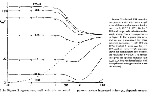
Figure 2 shows that this scaling rule actually holds with our model. For a number of pairs of scaled parameters ST and rT, which were taken from a region

5 ST

5

lo2 and 0

S

TT S lo2, we calculated pess

for three different durations T = 100, 320, and 1 0 0 0 .

For a fixed value of Y T , the scaled results peS7 as a function of scaled parameter ST lie reasonably well on

a curve notwithstanding different T ’ S were used.

T h e curve for T-T = 0 (complete linkage) corre-

sponds exactly to the contour line of evolution rate v = p of a continuous time replicon model under a periodic selection corresponding to our (7) (Figure 3 of ISHII, MATSUDA and OGITA 1982). This is as it should be. According to the extended Haldane-Muller principle of mutation load &/dp = 1

-

u / p (ISHII and

MATSUDA 1985), v / p = 1 corresponds to pop which

maximizes the long-term average Gz of averaged Mal- thusian parameter ( i e . , dG/dp = 0).

Figure 2 shows that for a fixed rT, p e s s ~ does not depend on ST as long as ST 5 1 . As we further increase ST, peSs7 decreases to a certain minimum less than 1 ,

and then increases to 1 asymptotically in the limit of large ST. However, for TT S 1, the asymptotical ap-

proach of p e s s ~ to 1 from below is not so conspicuous as for r~

>>

1 .

The fact that pess = 1 / ~ for very strong selection has been known for completely linked modifier case r =

0 by LEIGH (1970). Figure 2 shows that it applies also

for unlinked modifiers although the required ST is the

greater for the larger T T . For very strong selection s

= 1 , it can be further shown by our formula (4) that

pess is always equal to the reciprocal of the average duration of environment, whether the fluctuation is periodic or random (see APPENDIX

c).

T h e level of pew7 for small ST can be calculated

analytically by assuming that for such weak selection the frequency of A allele at the main locus fluctuates only near around 0.5. By a linear analysis based on expansion of A frequencies around 0.5, we obtain in

1

+

e- R-2M

(

R

+

2M R 1

+

e-2M

)

APPENDIX B.

1 1

-

e-R-2M 1

-

e-2M

-2-

1 1

-

e-2M

+-

- - = l o

2M 1

+

e-2M 2

(5)

Evolutionarily Stable Mutation Rate 167

1 in Figure 2 agrees very well with this analytical result.

Figure 2 also shows that peSs7 for a fixed ST mono-

tonically decreases as r7 increases from 0. However, the decrease is not large as long as rr 5 1, and becomes appreciable only for r7

>

1.

T h e fluctuating selection

(7)

can be said to be with a single strong Fourier component (i.e., sine wave component) since its frequency spectrum has a single strong peak at the frequency w = P / r . However, there remains a question if the above result obtained for this specific case really gives us a good general picture of pes, in a fluctuating environment with a single strong Fourier component. Although we can not be very conclusive, the answer seems to be yes. For example, we may consider a purely sine wave fluctuation

S(t) = S COS(Pt/T

+

'P) (8)

as a second environment. Here, s denotes the strength of selection, 7 is the number of generations during

which one allele is persistently favored than the other, and 'P is the phase parameter of the environment. As we show in APPENDIX B, in the weak selection limit this environment gives p , , ~ which is nearly equal to 7r/2 for rr

<<

1, and ?r2/2r7 for r7

>>

1. This is essentially the same result as explained in the above for the corresponding environment

(7).

Numerical solution of (4) for this environment shows that the behavior of p , , ~ for ST

>

1 is also similar to that of

the corresponding environment (7).

Fluctuation with multiple Fourier components:

For a fluctuation consisting of multiple Fourier com-

FIGURE 2,"Scaled ESS mutation rate p-7 us. scaled selection strength ST for different scaled recombination rate YT = 0 , ~ o - O . ~ , 1, 10,

100 under a periodic selection with a single strong Fourier component as in Figure 1. For a given pair of ST

and Y T , p., is calculated for three

different durations T = 100,320 and 1000. Symbol

+

gives p L . , ~ for T =

100, symbol

-

for T = 320. Lines are drawn for each fixed YT as to connect the results for T = 1000. The broken line gives the optimal mutation rate

pop as pOp7 for a random selection with

strengths and average duration r (see DISCUSSION).

IO IO0

ponents, we are interested in how pess depends on each component. As a simplest example, let us consider a two component case where s ( t ) is the sum of two periodic sequences as are given in

(7)

respectively with strength and duration SI, 7 1 and S P , 7 2 . Denoting by

p& the ESS mutation rate for a periodic selection with a single strong Fourier component of strength si and

duration 7i, we introduce the relative deviation 6 =

(pess

-

pi2)/(pi2

-

pi::) of pess from

pg.

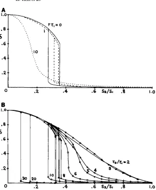
6 = 1 and 6 =

0 mean that the most effective component in determining we, is the first and the second one, respectively. Figure 3A shows how 6 changes as ~ 2 1 . ~ 1 increases from 0 to 1. T h e first component is fixed as s l r l =

lo-' with 7 1 = 3 1. T h e second component is chosen

to have a fixed duration 7 2 = 3 10. Calculations were done for rT1 = 0, 1 and 10. It should be noticed that the strength of the second component changes from s272 = 0 to as s2/s1 increases from 0 to 1, and three levels of linkage correspond to rT2 = 0, 10, 100.

Since s171

<<

1 and s272

<<

1, pi:! and pi:! are almost independent of the selection strength and are essentially determined by r71 and r72, respectively.

As sz/sI increases from 0 to 1, pess always decreases monotonically, whether the modifier is linked or not. It starts from pit! (6 = 1) and lies above pi:! (6

>

0). T h e mode of decrease, however, seems to make a change from sharp transition to gradual decrease as the modifier becomes more loosely linked with the main locus.

(6)

K. Ishii al.

I

FIGURE 3.-A, The ESS mutation rate pes us. the relative strength s2/sl of selection for a periodic selection with two strong Fourier components. The shorter duration component is fixed as s l ~ l = lo-’ with T~ = 31. The longer

duration component has a fixed duration 7 2 =

310. The ordinate is the relative deviation b = bSs - p$?)/(pC!:!

-

PC!?) of pes from

A?,

where P%

is the ESS mutation rate for a periodic selection with a single strong Fourier component of strength s, and duration 7,. The solid line is for

the recombination rate r = 0 between the modifier and the main loci, the broken line for m 1=

1 , and the dotted line for = 10. B, The low pass filter effect on ks for a periodic selection with two strong Fourier components us. the relative duration 7 2 / 7 1 = 2, 3, 4, 5, 6, 8, 10, 20, 30.

Calculation is for the case of completely linked modifiers ( r = 0). The shorter duration component is fixed in the same way as in A. The ordinate and the abscissa are taken in the same way as in A.

A

1.a

. 8

6

.6

* 4

.2

0

6

f

1.0 .4

.2

0

I 0

.2

\

d S ~ / S I 5 0.358, it consists of two branches giving two

locally stable pess’s. At s2/s1 = 0.281 a sharp drop of 6

occurs to start its lower branch, and at s2/sl = 0.358 another sharp drop occurs to end its upper branch. Since the lower branch of 6 lies below 6 = 0.05, we may say that the longer duration component is mainly responsible in determining pes if s2/sl exceeds 0.358.

Thus, our result for the complete linkage case is in accordance with what SASAKI and IWASA (1987) found and named as the low pass filter effect as for the optimal recombination rate in a fluctuating environment with multiple Fourier components.

T h e low pass filter effect is observed also for unlinked modifiers. For T71 = 1, &?71 = 1.32 and p% = 0.483. Recombination does not reduce pi:? appre- ciably, but reduces

&!

significantly since r ~ 2 = 10

>>

1. Even in this case, we see that 6 is less than 0.05 for

s2/sl

L

0.35. For rT1 = 10, &?71 = 0.402 and piz?72 = 0.049. Recombination reduces both and

&

significantly. In this case, 6 is less than 0.05 for S ~ / S I

L

0.43. However, the transition into the regime where the longer duration component dominates in determining pes is not so sharp as for T T ~

5

1 cases.

Figure 3B shows 6 for r = 0 case versus the relative strength s2/sI for different 72/71 = 2, 3, 4, 5, 6, 8, 10,

20, 30. T h e first component is fixed just in the same

way as in Figure 3A. 6 is less than 0.05 for s2/sl

2

0.5

if and only if 72/71

>

5. For a given 72/71, 6 decreases

only gradually with s2/s1 for 72/71 d 5, but it makes

sharp drops for 72/71

>

5. The first drop of 6 which

starts its lower branch occurs at the smaller s2/s1 value

for the greater 72/71. However, the second drop of 6

which ends its higher branch occurs at an s2/s1 value

(between 0.25 and 0.4) which does not change very much with 72/71.

Combining the results in Figure 3, A and B, together, we can conclude that the low pass filter effect works generally for 72/71

>

5 and for S ~ / S I 2 0.5,

whether the modifier is linked or not.

DISCUSSION

In this paper we examined the evolution of mutation rate controlled by neutral modifiers by a formula (4) for the evolutionarily stable mutation rate pess. T h e main results obtained in previous sections are sum- marized as:

I. For any fluctuation, periodic or random: (1) if the recombination rate T per generation between the

(7)

and

(2)

for any r , if the strength s of selection per generation is very large, pes is equal to the reciprocal of the average number T of generations (duration

time) during which one allele is persistently favored than the other.

11. For a periodic fluctuation in the limit of small s

and r , pes,? is a function of ST and rT with properties:

(1) for a given S T , peSs7 decreases with increasing rT;

(2) for ST 5 1, peSs7 is almost independent of S T , and

depends on rT as &,T = 1.6 for rT

<<

1 and peS,7 =

6/r7 for rT

>>

1 ; and (3) for ST

2

1, and for a given

rT, p , , , ~ decreases with increasing ST to a certain min-

imum less than 1, and then increases to 1 asymptotically in the limit of large S T .

111. For a fluctuation consisting of multiple Fourier components ( i e . , sine wave components), the component with the longest period is the most effective in determining pes, (low passfilter effect).

O u r results should be compared with those of LEIGH (1970). Based on an analysis which is valid for very strong selection, he claimed that in an asexual population selection adjusts the mutation rate toward a nonzero level which is equal to the reciprocal of the duration of fluctuating environment. Based on the general ineffectiveness of intergroup selection, he further argued that in a sexual population selection on mutation rates would operate toward zero. Our result (12) is in accordance with LEIGH’S claim about an asexual population, and (113) extends it to the general case of s

>>

1 / ~ . However, our result does not support LEIGH’S claim about a sexual population, since pes, is always positive in a periodic environment for any value of recombination rate r .

Invadability of an ESS modifier: In this paper we

analyzed the evolutionary stability of a wild-type modifier against an invading modifier only at its initial stage of invasion. However, even if the invading modifier is successful when its frequency is low, it may not be so when its frequency becomes higher. In that case, the wild type modifier which is not ESS in the sense of our present analysis can persist to exist by somehow controlling the invading modifier at a low frequency level in the population. From this point, an interesting question is whether an ESS modifier with pes, # pop

can invade into a population of pop with the greatest average population fitness.

We studied this by a computer simulation of the whole process of modifier competition for typical cases. We found that an ESS modifier always suc- ceeded in invading into the population of a non-ESS modifier (chosen from the attractor of the studied pes,, when more than one local ESS modifiers existed). This gives a support to our expectation that the mutation rate will evolve toward pes as is calculated in this paper.

Random fluctuation: In the real environment some

stochastic elements are usually included in its fluctuation. So, let us consider what kind of differences will be expected in a randomly changing environment. In this case an explicit analysis of formula (4) for pes is not so easy because X(p’, p ) in a random environment is difficult to evaluate explicitly. However, our results in (I) apply generally whether the environment is random or periodic.

Thus, if the modifier is completely linked, pes is equal to pop. For a simple model of random environment in which the selection coefficient s(t) makes a Markov process which takes two values +s and -s with an average duration T, pop can be obtained directly by maximizing the long-term geometric average of population fitness which we can evaluate numerically based on an explicit result on the stationary distribu- tion of allele A at the main locus (MATSUDA and ISHII

1981). T h e result pop^ is shown in Figure 2 by a

broken line. Comparing two curves of pop for a random environment and for a corresponding periodic one, we see that they are approximately at the same level for ST

>>

1. This is as is expected from our result

(1

2).

However, for weak selection ST

<<

1, we see that pop in a Markov environment approaches zero as pop = 0.5s while pop in a periodic environment stays at a finite level of 1.606 1 / ~ . T h e smaller pop for a random environment than for a periodic one may be explained by the low pass filter effect as due to the longer period Fourier components of fluctuation which are contained in a random environment.

For the loosely linked modifier case, we can show, in a similar way as in APPENDIX B, that pes in the above mentioned Markov environment is at most less than 10s in the weak selection limit (ST

<<

1). Further, since

we have low pass filter effect also for unlinked modifiers, we may expect that pes, for a random environment is generally smaller than that for a corresponding periodic environment, and that the difference will be the greater for the weaker selection. This expectation was borne out by computer simulations of the modifier competition.

Using a diffusion approximation GILLESPIE (1 98 1) studied the evolution of mutation rate by a modifier model with the selected locus under a fluctuating selection which generally brings about a marginal overdominance. Our model in the above mentioned Markov environment corresponds in the weak selection limit ST

<<

1 to his diffusion model with parameters A = 0 and B = 1 (MATSUDA and ISHII 1981), for which his result is that selection will continue to increase the mutation rate whatever its current value. This result is at variance with our above result of pes,

1 Os. Since the diffusion approximation used by him is justifiable only for ~ / s ’ T = 0 (1) in the limit of s +

(8)

p such as p/s = 0 (1). We presume that this is the cause of the discrepancy.

Cost of preventing mutation: In this paper we have

assumed that mutation rate modifiers are selectively neutral, but they can not be always neutral for real organisms. In order to reduce the mutation rate, it may be necessary for organisms to develop a replication system where the replication error is reduced. This necessarily requires more time and free energy for replication, causing a decrease in the multiplication rate of organisms per unit time. Then, pess es- tablished by such non-neutral modifiers is expected not to be so low as by neutral ones.

As a simple model of non-neutral modifiers, let us consider a multiplicative two-locus model with a modifier of mutation rate p contributing a fitness compo- nentf(p). Then, the formula (4a) is modified as

4 P ) / V / J , CL)

+

C(P) = 0. (4a') Here, c(p) sf '(p)/'(p) is the relative cost to reduce mutation rate by a unit amount, and can be assumed to be non-negative. Then, for c(p)

>

0 formula (4a') gives pes, larger than in the case of neutral modifiers

(c(p) = 0) under the same selection pressure acting at the main locus.

If the modifier is loosely linked with the main locus, we found that pes, by neutral modifiers is smaller than the optimal rate pop. Then, we may ask how much cost c* is needed to increase pes, to the level of pop of the neutral modifier case. According to (4a'), c* is

Figure 4 shows for the periodic selection

(7)

how the critical cost c* depends on the scaled model parameters ST and 7-7. For a given s7, c* increases with increasing YT from c* = 0 at 7-7 = 0 to a certain maximum E * , and then decreases to 0 asymptotically in the limit of large rT. Curves for different ST values

less than 1 are of the same shape but are proportional to (ST)'. T h e maximum E* for a given s7 depends on ST d 1 as E* = (s~)'/100. For 1 S s7 d lo6, E* gradually

increases with increasing ST but stays less than 1. The

behavior of c* for s7 d 1 can be explained by the result of APPENDIX B for the weak selection limit.

Based on an extended Haldane-Muller principle of mutation load, ISHII and MATSUDA (1985) proved that, if there is no cost of preventing mutation, pop is equal to the evolution rate u which is defined as the increase rate of population average of mutation numbers which have occurred along the phylogenic line leading to the present replicons. They further showed that u

<

pop if there is a positive cost of preventing mutation, and pointed out that this may explain, from a selectionist perspective, the fact that molecular evolution rates are smaller than total mutation rates. Their argument assumed completely linked mutation rate modifiers, but can be extended to the case of unlinked modifiers as ZI

2

pess for c*

2

c. Thus, the given by -A(Pop)/YPop' Pop).

above mentioned fact about molecular evolution rates corresponds to the case when the unlinked modifiers incur a positive cost c of preventing mutation greater than c*. When some reliable data are obtained in the future about how large is the cost c, it can be compared with the values of c* given in Figure 4.

Two allele model under fluctuating selection: Our

model assumes at the main locus that mutation occurs between two alleles, and that they become the more fit than the other alternatively. This assumption is very suitable for the$$-fop mutation in bacteria and bacteriophage (WATSON et al. 1987).

For example, individual Salmonella bacteria can alternate flagella protein expression between two types, H1 and H2, which differ in antigen property. Since the flagella protein is a dominant antigen of Salmonella, the switching is favorable in eluding the host immune defense. T h e molecular mechanism has been clarified (BORST and GREAVES 1987): In one phase of gene expression, the gene for H1 is transcribed together with an adjacent gene that codes for the repressor of gene for H2"hence only H1 is expressed. In alternative phase, the promoter sequence of H1 is inverted, and neither H 1 gene nor repressor gene for H2 is transcribed, then only H2 gene is expressed. T h e orientation of the invertible segment thus determines gene expression of flagella protein. The rate of occasional inversion of the segment is regulated by the recombinase, Hin, which is coded within the segment itself, together with promoter sequence of H 1. Hence, this is an example of completely linked mutation rate modifier in our model.

Another mechanism for switching between two alleles is a cassette mechanism for the mating type of yeast (DARNELL 1982). It is known that there are two silent loci together with a single expression locus. T h e expression locus is occasionally renewed by gene con- version from one of the two silent loci in which the information is stored.

If the rate of flip-flop in bacteria or mating type change in yeast is to be evolutionarily determined, our model gives the rate which is to be realized as a result of evolution.

General interpretation of the two-allele model-

parity model: At first sight, or taken literally, the two-

(9)

FIGURE 4.-The critical cost c* of preventing mu- tation that is needed to increase to the level of of the neutral modifier case. The same periodic selec- tion with a single strong Fourier component as in Figure 1 is assumed. The scaled result for c* is calcu- lated for a given pair of scaled parameters ST and rT

with T = max(lOs7, 1 0 ~ ) . Lines are drawn for each

fixed ST value.

lem of mutation rate may be very limited unless the modifier locus is extremely site specific in its actions.

We do not deny the possibility that many mutations will be deleterious in essentially all environments, yet we consider that models studied in this paper may still represent some essential feature of the real replication unit (replicon) such as a chromosome or

D N A

by the following reasons.

We have assumed only two alleles at the main locus, but their fitnesses are generally time-dependent. Then, by classifying all the possible genetic states of

replicons into just two types, we can regard the above fitness as an average fitness of a subpopulation consisting of the respective type of replicons. In that case, the fitness of replicons which are deleterious in every environment will be considerably low, so that their frequencies will remain very small in each subpopu-

lation. Then, their effect on the average fitness of each subpopulation will also be small.

Therefore, under a suitable dichotomous classification of genetic states, it may be possible that the average fitness of each type fluctuates essentially like the model we have considered in this paper. If this is indeed the case, the mutation rate modifier need not be site specific in order for our model to be applicable.

For instance, we may classify four kinds of bases

A,

T, G, and C into purines

(A

or G) and pyrimidines (T

or C). Then, we may classify the base sequences of

D N A

according to whether the total number of purines contained in each sequence is even or odd. It is like the classification of the internal states of elemen- tary particles by even and odd parity.

(10)

K. et al.

models with general interpretation as may be called a “parity model” will be worthwhile.

We thank S. KASHIWAMURA and J. ISHIMOTO for helpful comments on an earlier version of this paper. We also thank anonymous reviewers of this paper for helpful comments to improve the pres- entation. This work was supported in part by a Grant-in-Aid for Special Project Research on Biological Aspects of Optimal Strategy and Social Structure from Ministry of Education, Science and Culture.

LITERATURE CITED

BORST, P., and D. R. GREAVES, 1987 Programmed gene re- arrangements altering gene expression. Science 235: 658-667. DARNELL, J. E., JR., 1982 Variety in the level of gene control in

eucaryotic cells. Nature 297: 365-370.

ment. Evolution 35: 468-476.

GILLESPIE, J., 1981 Mutation modification in a random environ-

ISHII, K., and H. MATSUDA, 1985 Extension of the Haldane- Muller principle of mutation load with application for estimat- ing a possible range of relative evolution rate. Genet. Res. 4 6 75-84.

ISHII, K., H. MATSUDA and N. OGITA, 1982 A mathematical model of biological evolution. J. Math. Biol. 14: 327-353. KIMURA, M., 1960 Optimum mutation rate and degree of domi-

nance as determined by the principle of minimum genetic load. J. Genet. 57: 21-34.

KIMURA, M., 1967 On the evolutionary adjustment of sponta-

LEIGH, E. G., 1970 Natural selection and mutability. Am. Nat.

LEIGH, E. G., 1973 The evolution of mutation rates. Genetics 73 neous mutation rates. Genet. Res. 9 23-34.

104: 301-305.

(Suppl.): sl-s18.

LEVINS, R., 1967 Theory of fitness in a heterogeneous environment. VI. The adaptive significance of mutation. Genetics 56: 163-178.

LIEBERMAN, U., and M. W. FELDMAN, 1986 Modifiers of mutation rate: a general reduction principle. Theor. Popul. Biol. 3 0 125-142.

MATSUDA, H., and K. ISHII, 1981 Stationary gene frequency dis- tribution in the environment fluctuating between two distinct states. J. Math. Biol. 11: 119-141.

MAYNARD SMITH, J., and G. R. PRICE, 1973 The logic of animal conflict. Nature 246: 15-18.

SASAKI, A , , and Y . IWASA, 1987 Optimal recombination rate in

STURTEVANT, A. H., 1937 Essays on evolution. I. On the effects of selection on mutation rate. Q. Rev. Biol. 12: 464-467. TAKAHATA, N . , K. ISHII, and H. MATSUDA, 1975 Effect of tem-

poral fluctuation of selection coefficient on gene frequency in a population. Proc. Natl. Acad. Sci. USA 72: 4541-4545. WATSON, J. D., A. H. HOPKINS, J. W. ROBERTS, J. A. STEITZ and

A. M. WEINER, 1987 Molecular Biology of the Gene, Vol. 1, Ed. 4. Benjamin/Cummings, Menlo Park, Calif.

fluctuating environments. Genetics 115: 377-388.

Communicating editor: D. CHARLESWORTH

APPENDIX A

Method of numerical analysis of (4)

as

First, let us write down the characteristic equation of MT

X’

-

XTrkfT

+

deMT = 0. (A1 )

Its greatest eigenvalue X@’, p ) is given by

X(p’, p) = (TrMT J(TrMT)‘

-

4 d e t M ~ ) / 2 . (A2)

Then, differentiating (Al) with p ’ , we have

(2X

-

TrMT)dX/dp‘

-

XdTI“T/dp’

+

ddeaT/dp’ = 0, which gives

dX(p’, p)/dp’= (XdTrMTldp’

(‘43)

-

ddetMT/dp’)/(2X

-

TrMT). Thus, in order to calculate by (A2) and (A3) the value of

A(p) = [dX(p’, p)/dp’],,,=,, for a given p , we need only to know four values at LC’ = I.L of TrMT and deMT together with their partial derivatives with respect to p‘. and dTrMT/dp’ are immediately obtained once matrices MT and dM~/d/.t‘ are numerically calculated by the following iteration

Mf+I = M(t)M,, (-444

and

dMt+l/dp’ = M(t)dMc/dp’

+

[aM(t)/+’]Mt (A4b)

for t = 0, 1,

. . .

, T

-

1, where d M ( t ) / d p ’ is calculated from

(2) as

- -

dM(t)/dp’ = (1

-

r,

L

1

+

s ( t ) -1

+

s(t)

1 .

(A5)

-

1

-

s(t) 1

-

s ( t )

detMT is calculated from (2) and (6) as

detMT = ((1

-

r)(l

-

2p’))’’

n

( 1

-

s(t)’), ( A 6 4

7” I

l=O

with

ddetMT/dp‘ = -4rdetM~/(1

-

2p’). (A&)

Calculating necessary p’ derivatives by (A4)-(A6), we

obtain by (A2) and (A3) the value of A ( p ) for each p. Finally, zeros of A ( p ) in the range [ 0 , 13 are obtained by a routine of bisection.

APPENDIX B

pess in the weak seletion limit

In this appendix we show how we can analytically study perr when the frequencies x ( t ) and y(t) of A alleles, respectively, among B carrying genomes and among b carrying ones, keep fluctuating only very near around 0.5. Such a situation is realized when the strength s of selection is very small compared with the mutation rate p.

First, we restate the condition (4) for peSs in terms of x ( t ) andy(t). Since the average fitness G(t) of 6 carrying genomes is expressed as G(t) = 1

+

s ( t ) ( Z y ( t )

-

1) in terms of y(t) = N l ( t ) / N ( t ) , the increase rate X(p’, p ) as the long-term geometric average of G(t) is given in the weak selection limit as

X@’, p ) = 1

+

lim t-’ s ( t ’ ) { Z y ( t ’ )

-

I ) ,

where w e have neglected higher order terms of s. Compar- 1- 1

(11)

Evolutionarily Stable Mutation Rate 173

ing this with the rate k(p, p ) for B carrying genomes, which is obtained by replacing y(t’) with x(t’

-

1) in the above, we find

I- 1

for p’ # p

as the condition for p to be a pes.

From (1) and (2), the time change of y(t) is given by

y(t + 1) = EIrx(t)

+

(1

-

r)(l

-

r’)l{l

+

s(t)Jy(t)

+IrJc(t)+(l -r)cLtlI1 -s(t)lll -y(011/[1 +40i2y@)- 111.

The time change of x ( t ) is given by (3) since x ( t ) = x,@). By assumption, the deviations of x ( t ) and y(t) from 0.5 become small magnitude quantities after a finite transient period. Therefore, by expanding x ( t ) and y(t) around 0.5 and keep- ing only the leading terms in the equations for the time change of x ( t ) and y(t), we find that [(t) = x(t

-

1)

-

0.5 and f i t ) = y(t)

-

x(t

-

1) become to satisfy

and

T(t

+

1) = (1

-

r)[-(Cc’

-

P ) b ( t )

+

2f(t)l

(B3)

+

(1

-

2 d )

T(0l

to the lowest order terms of s.

Alternating environment with duration T: We consider a periodic selection with s ( t ) given by (7). From the assumed symmetry of s(t), [ ( t ) and nt) converge to the periodic sequences which satisfy [ ( t

+

T ) = - f ( t ) and T(t

+

T ) = - f i t )

for any t . Then, the average ({s) in (Bl) is calculated as

7-1

in terms of a sequence {T(t); t = 0, 1,

. . .

, T J which is the

solution of constant coefficient equations

[ ( t + 1 ) = ( 1 - 2 p ) ( ~ / 2 + ( ( t ) J ( t = 0 , 1 , . . - , ~ - l ) (B5)

and

from the boundary condition. Then we substitute (B7) in (B6) and find T(t) in the limit of p‘ 4 p as

T(t)=((1-r)(l-2p)JfT(0)+(1-r)s- P’ - P CL

1 -(1 -ry (1 -2py

.[

r 1+(1-2p)7

” 1 l - ( ( l - r ) ( l - 2 p ) ) f

2 l - ( l - r ) ( l - 2 p )

where T(0) is determined as

1 -(1 - r y (1 -2py

.[

r 1+(1-2pY

” 1 1

-

((1

-

r)(l

-

2/41‘

2 1 -(1 -r)(l -2p)

1

from the boundary condition. Substituting (B8) in (B4), we finally obtain ({s) as

with

1 / 7

f ( p ’ r ) = 1 + [ ( 1 - r ) ( l - 2 p ) J T

1-((1-~)(1-2p))’ 1-(1-r)’ (1-2p)’

* [ 1 -(I -r)(l-2p)

- 2

r 1 +(1-2p)‘

1 - 2 p 1 -(1-2$ 1

+-

2 ~ p 1 + ( 1 - 2 p y 2’

”

According to the result (B9a) for ({s), the condition (Bl) for p to be a pes becomes asf(p, r) = 0 for 0

<

p < 1, and

f( 1, r ) 2 0 for p = 1. The result (B9b) forf(p, r ) then shows that p = 1 is a k s if and only if T is an odd integer. We

further see thatf(p, r)

>

0 for 0 < p < 1 if T = 1, and that

f ( p , r ) = 0 only for p = 0.5 among 0 < p < 1 if T = 2.

Therefore, in the weak selection limit, p = 1 is the only pear for T = 1, and p = 0.5 is the only one for 7 = 2. For T Z 3,

f ( p , r ) = 0 has a root in 0 < p < 1, giving a pes which

generally depends on two parameters T and r . These results

explain the numerical results for ST 5 1 in Figure 1.

We next show how the last mentioned p,,, becomes to satisfy a scaling rule for T > 1. We fix C(T = M and r~ = R

at finite values and let T 4 m. Then, we find F (M, R) = limf(MI7, R/T)

7-

-

( l

-

e-R-2M

1

-

e-R e-2M

1

+

R

+

2M -2” R 1

+

e-2M

)

(B10) 1 1

-

e-2M 1 +“”

2M 1

+

e-2M 2‘

For a given R = 7-7, F(M, R ) as a function of M has a zero M

> 0 which gives the scaled pesa7. In a special case of R = 0,

which corresponds to the completely linked modifier case, F(M, 0) = 0 is numerically solved to give M = 1.606 1

. . . .

In the opposite case of R >> 1, which corresponds to the loosely linked modifier case, M << 1 satisfies M/R

-

M2/6 =

(12)

results for ST 5 1 in Figure 2. There, we further note that

p e r r ~ for a fixed rT is independent of ST not only for s < p but also for s B p as long as ST 5 1. This suggests that

periodic selection for ST < 1 also can produce an additional

drift of x ( t ) toward 0.5 just as is known for stochastic selection (GILLESPIE 1972; TAKAHATA, ISHII and MATUSUDA 1975).

Sinusoidally oscillating environment with period 27: We now consider a second example of periodic selection with

s(t) given by (8). This environment is similar to the previous one in that one allele is persistently favored than the other for T generations. Noting that cos(wt

+

P) = Re(e<"'+')), we

assume the deviation of frequencies as { ( t ) = Re(sXei("Lw)) and fit) = Re(sZei(w'+')) with w = T / T . Then, the average in

(BI) is calculated as ({s) = s2Re(Z/2), while the complex amplitudes X and Z satisfy from (B2) and (B3)

Xe'" = (1

-

2p)(1/2

+

X) (B1 l a )

and

Ze" = (1

-

r)(-(p'

-

p)( 1

+

2X)

+

(1

-

2p')Z). (B1 l b ) After some calculation we obtain in the limit of p' + p

-

2(1

-

2p)cos w ) X ( 1 + (1

-

r)'(1

-

2 ~ ) ~ (B12a)

-

2(1

-

r)(l

-

2p)cos a]]

with

(B 12b)

-

((1

-

r)(l

-

2p)2

+

1 ]cos w .

According to the result (B 12a) for ({s), the condition (B 1) for p to be a pess becomes as g(p, r ) = 0 for 0 < p < 1, and g( 1, r ) B 0 for p = 1. T h e result (B 12b) for g(p, r ) then shows that p = 1 is a pes if and only if T = 1. We further see

that g(p, r ) > 0 for 0 < p < 1 if T = 1, and that g ( p , r ) = 0

only for p = 0.5 among 0 < p < 1 if T = 2. Therefore, in

the weak selection limit, p = 1 is the only pes for T = 1, and

p = 0.5 is the only one for T = 2. For T

B

3, g(p, T ) = 0 has a root in 0 < p < 1, giving a pes which generally depends on two parameters T and r .

T h e scaled result for this environment is given by

G(M, R) = 0 with

G ( M , R ) = Iim T2g(M/T, R/T)

7-

= a2

-

2RM

-

4M2. (B 13)

Thus, we find M =

(n

-

R)/4. This gives M =

a/2 for R << 2a, and M = r2/2R for R >> 2a. It should be

noted that the results for this environment are essentially the same as those for the corresponding alternating environment.

Continuous time models: If we are interested only in the scaled results obtained in the above by taking a limit of T + 0 , it should be noted that they can be obtained more easily by starting directly from a continuous time model corresponding to our discrete time model (1) and (2). Then the rate X becomes equal to the long-term arithmetic average of the average Malthusian parameter 7iL(t) of b carrying genomes in a population dominated by B carrying ones. T h e linear analysis based on the expansion of frequencies around 0.5 can be easily carried out in a similar manner as has been explained in the above for discrete time models.

APPENDIX C

pes* under very strong selection

In this appendix we consider a fluctuating selection where

s(t) takes only two values +sand -s with an average duration

T . T h e fluctuation may be either periodic o r random.

Under very strong selection with the strength of selection

s very near to 1, we find that the frequency x(t'

-

1) of A alleles among B carrying genomes, just before recombination takes place in the (t'

-

1)th generation, is 1 - p o r p according to whether s(t'

-

1) is +s o r -3. Then, the

frequency y(t) of A alleles among b carrying genomes, just before selection takes place in the tth generation, is y+ = r( 1

-

p )

+

(1

-

r)(l - p ' ) o r y- 1

-

y+ according to whether s(t'

-

1) is +S o r -s. Therefore, the average fitness

G ( t ) = 1

+

s(t)(2y(t)

-

1) of b carrying genomes is 2y+ or 2y- according to whether s ( t ) = s(t

-

1) o r not.

Since the environment continues to be the same for T

generations on the average, we find that the rate X(p', p ) as the long-term geometric average of G(t) is given by

log X(p', p) = log 2

+

(logy-

+

(7

-

1) log y + ) / T .

Substituting this in (4), and noting that

A(P) = (1

-

r P ( 1

-

TP)/TP(~

-

P ) ,

we obtain pes = 1 / ~ for any recombination rate r between the modifier and the main locus.

It can be shown in a similar way that the same result as above holds also for the following more general situation. We assume that there are a finite number a of alleles at the selected locus with the fitness of allele A, given by 1

+

s i ( t )

and the mutation rate from Ai to Aj given by pfij, where p is the total mutation rate specified by an allele at the modifier locus andfij is a non-negative constant satisfying

Cfij

= 1 .