Spatial Aggregation and Prediction in the Hedonic Model

(1)

FULCHER, CHARLES MICHAEL. Spatial Aggregation and Prediction in the Hedonic

Model. (Under the direction of Raymond Palmquist).

Using a data set of Wake County, North Carolina, property sales for the period

1992-2000, this study provides evidence as to the acceptability of spatial aggregation in

hedonic property value models. Both statistical tests and tests based upon prediction errors

are performed in order to identify the circumstances under which aggregation is statistically

acceptable or acceptable from a practical standpoint. This study makes extensive use of

spatial econometric techniques in order to control for the spatial correlation problems which

exist in models where location matters, and discusses the importance of speciﬁcation and

functional form as determinants of both the acceptability of aggregation and predictive

power. Since multiple speciﬁcations and types of models are estimated, this study also

provides guidance as to the type of model or speciﬁcation providing the best performance

when used to estimate hedonic property value models.

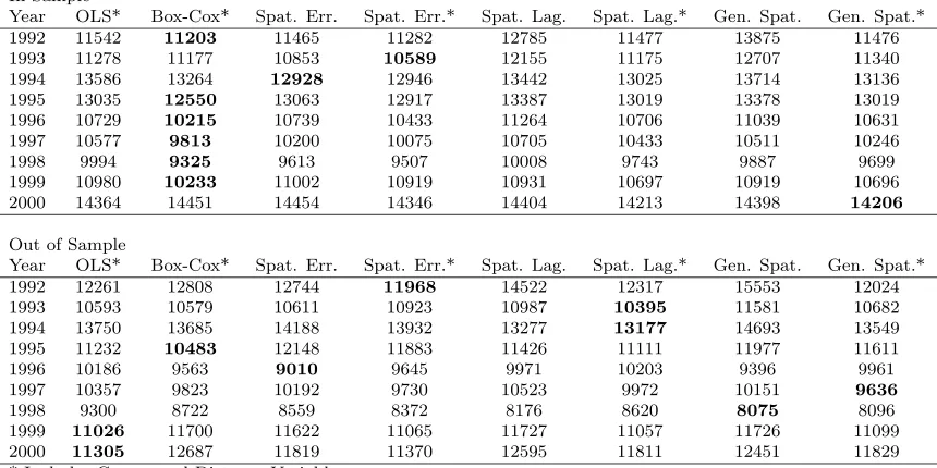
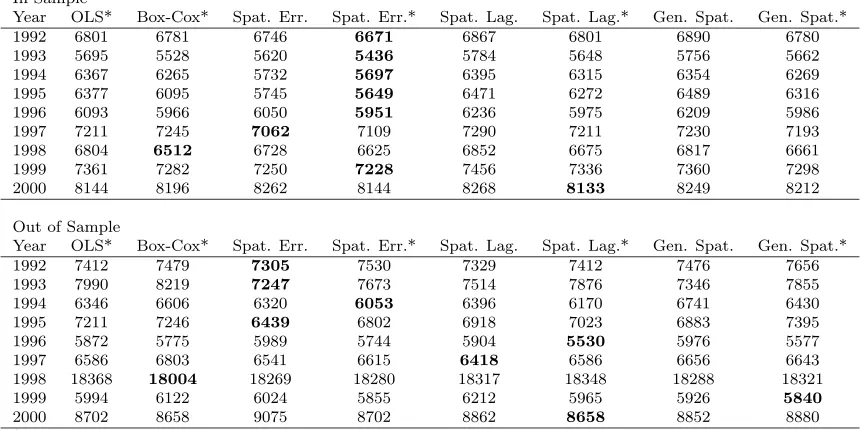
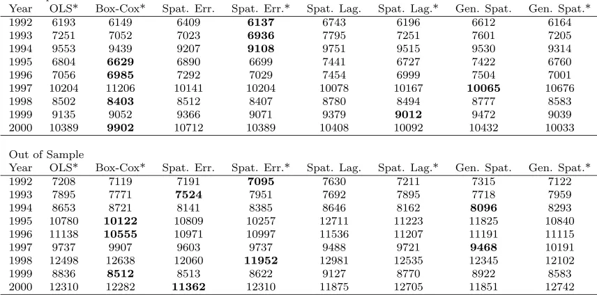
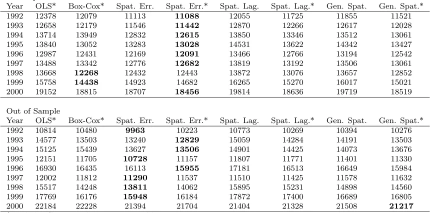
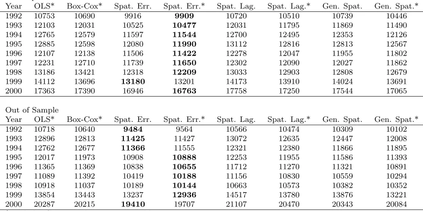
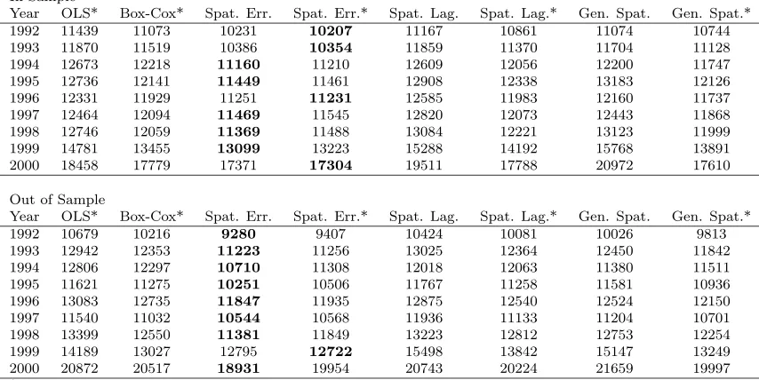
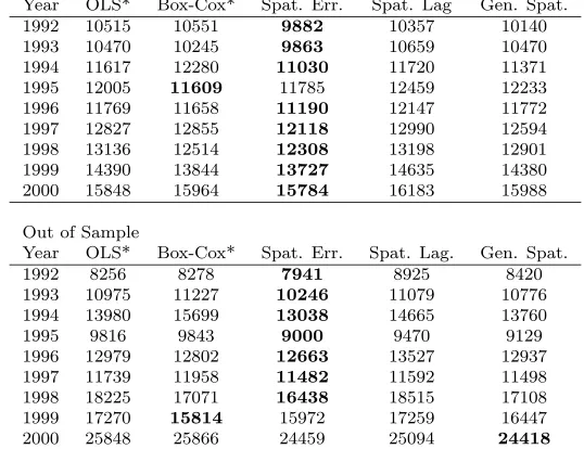
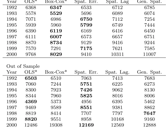
The primary ﬁnding of this study is that while statistical tests typically reject

ag-gregation, the eﬀects of aggregation upon prediction errors is negligible. We would typically

expect less than a 2000 dollar increase in mean absolute prediction error from aggregating

the entire county, while in several cases the out-of-sample predictions would be improved.

Further, in many cases aggregation yields more plausible coeﬃcient values, especially for

less important determinants of property values. These results may indicate that aggregation

is preferable to extensive disaggregation when conducting hedonic property values studies,

especially if one is concerned with the coeﬃcient estimates. I also ﬁnd that a spatial error

model is typically preferred over OLS and Box-Cox alternatives, even when those

alterna-tives include additional variables describing the locational characteristics of the properties

(2)

by

Charles Michael Fulcher

A dissertation submitted to the Graduate Faculty of North Carolina State University

in partial satisfaction of the requirements for the Degree of

Doctor of Philosophy

Department of Economics

Raleigh

2003

Approved By:

Dr. Walter Thurman Dr. Michael Walden

Dr. Raymond Palmquist Dr. Stephen Margolis

(3)

(4)

Biography

Charles Michael Fulcher was born on May 26, 1972, to Michael and Betty Fulcher in

Mar-tinsville, Virginia. As a child he was often accused of being too smart for his own good

(a claim which has since been proven to be completely without merit) and proved to be a

source of constant consternation for his teachers. Nonetheless, in 1990 he graduated from

Fieldale-Collinsville High School as the valedictorian of his class, his last bit of academic

glory. After a thoroughly unimpressive four years at the University of Virginia, he

gradu-ated in 1994 with a double major in Economics and Foreign Aﬀairs. Seeking to make use

of both of these subjects, he then entered the International Economics Masters Program

at Radford University. While there, his interest in Economics was rekindled and, more

importantly, he met his future wife. In 1996, he entered the Economics Ph.D. program

at North Carolina State University, despite not having completed the requirements for his

Master’s degree. He corrected this oversight in 2001 and thus received his Master of Science

in International Economics. This cleared the way for the completion of his Ph.D. and the

(5)

Acknowledgements

First and foremost, I must thank my wife, Naoko, for her support and encouragement as

this dissertation took much longer than I had promised or she had expected. I can only

hope that I will be able to make it up to her someday. I must also thank Ray Palmquist

for coaching me through the intricacies of hedonic property value models. His invaluable

assistance made this research possible. Steve Margolis, Wally Thurman, and Mike Walden

also provided valuable guidance which helped shape this research. I am also grateful to the

Wake County Revenue Department for providing both ﬁnancial support and the data used

in this study.

Finally, thanks to my family and friends, especially John Deal, Aaron Hegde, and

Matt Roberts. They have all listened to more of my complaints than anyone should ever

(6)

List of Figures

(9)

List of Tables

6.1 List of Variables in Base Speciﬁcation . . . 42

6.2 List of Additional Spatial Variables . . . 42

7.1 Aggregation Test Results Summary . . . 53

7.2 SER Comparison Results Summary . . . 54

7.3 Prediction Error Comparison Results Summary . . . 57

7.4 Model with Lowest Mean Absolute Error . . . 57

7.5 Model Rankings Based on Mean Absolute Error . . . 58

7.6 Model Rankings Based on Mean Absolute Percentage Error . . . 59

7.7 Spatial Models vs. Extra Variables Lowest MAE . . . 60

7.8 Spatial Models vs. Extra Variables Rankings Based on MAE . . . 60

B.1 Aggregation Test Results for MLS Group 1 - OLS and Spatial Models . . . 76

B.2 Aggregation Test Results for MLS Group 1 - Box-Cox Transformations . . . 77

B.7 Aggregation Test Results for Wake County - OLS and Spatial Models . . . 82

B.8 Aggregation Test Results for Wake County - Box-Cox Transformations . . . 83

C.1 Comparison of SERs for MLS Group 1 . . . 85

C.4 Comparison of SERs for Wake County . . . 88

D.1 Comparison of MAEs for MLS Group A (Aggregated vs. Weighted Average) 90 D.2 Comparison of MAEs for MLS Group B (Aggregated vs. Weighted Average) 91 D.3 Comparison of MAEs for MLS Group C (Aggregated vs. Weighted Average) 92 D.4 Comparison of MAEs for Wake County (Aggregated vs. Weighted Average) 93 D.5 Comparison of MAEs for MLS Zone 1 . . . 94

D.6 Comparison of MAEs for MLS Zone 2 . . . 94

(10)

D.20 Comparison of MAEs for MLS Group A . . . 101

D.21 Comparison of MAEs for MLS Group B . . . 102

D.22 Comparison of MAEs for MLS Group C . . . 102

D.23 Comparison of MAEs for Wake County . . . 103

D.24 Comparison of MAEs for MLS Zone 1 (Spatial vs. Extra Variables) . . . . 104

D.39 Comparison of MAEs for MLS Group A (Spatial vs. Extra Variables) . . . 111

D.40 Comparison of MAEs for MLS Group B (Spatial vs. Extra Variables) . . . 112

D.41 Comparison of MAEs for MLS Group C (Spatial vs. Extra Variables) . . . 112

D.42 Comparison of MAEs for Wake County (Spatial vs. Extra Variables) . . . . 113

E.1 1992 OLS Estimates (Base Spec., All Observations) . . . 115

E.2 1992 OLS Estimates (Full Spec., All Observations) . . . 117

E.3 1992 OLS Estimates (Sparse Spec., All Observations) . . . 119

E.4 1992 OLS Estimates (Base Spec., Small Samples) . . . 121

E.5 1992 OLS Estimates (Full Spec., Small Samples) . . . 123

E.6 1992 OLS Estimates (Sparse Spec., Small Samples) . . . 125

E.7 1992 Spatial Error Estimates (Base Spec., All Observations) . . . 127

E.8 1992 Spatial Error Estimates (Full Spec., All Observations) . . . 129

(11)

(12)

Chapter 1

Introduction

Determining the extent of a market has long been an issue for practitioners

wish-ing to employ hedonic regression techniques. While it has been argued that the

delin-eation of homogeneous submarkets is necessary in order to accurately estimate coeﬃcient

values, there is considerable disagreement about how this delineation should be

accom-plished. While many studies have considered entire urban areas as a single market, other

researchers have suggested that much smaller areas should be used. At the same time, it

has not proven evident that extensive disaggregation is preferable, as many studies have

found non-plausible coeﬃcients when performing regressions on small areas. Further, there

is some evidence that disaggregation does not lead to greatly improved results if the goal

of the study is forecasting prices. The goal of any hedonic study is to accurately represent

the price schedule existing within a market, so the essential question is how large an area

can be used for estimation while still achieving this goal.

This study hopes to shed some light upon the issue of aggregation by identifying the

circumstances under which aggregation over space is statistically acceptable or acceptable

from a practical standpoint. I investigate the necessity of the spatial disaggregation typically

seen in hedonic studies and suggest methods that can deal with spatial correlation problems

as part of the estimation procedure. In addition, I discuss the importance of speciﬁcation

and functional form as determinants of both the acceptability of aggregation and predictive

power. Since multiple speciﬁcations and types of models are estimated in this study, it also

(13)

when used to estimate hedonic property value models.

This paper is organized as follows. Chapter 2 provides an introduction to the

economic theory underlying this study, speciﬁcally the household’s decision of where to live.

As part of this discussion, two of the major theories of housing location choice are presented.

These models provide a natural starting point for this study, as they emphasize the role

that location and housing characteristics play in the decision process. The hedonic method,

one technique often used in environmental and resource economics to assess the value of

particular housing characteristics, is also discussed and is the estimation technique used

throughout this study. The concept of market segmentation and its impact on estimated

coeﬃcient values is introduced and the relevant literature on market segmentation and

aggregation in the housing market is discussed.

Chapters 3 and 4 deal with modiﬁcations to the estimation procedures which may

be employed in order to account for spatial relationships occurring within the data, and to

introduce more ﬂexibility into the functional form of the estimating equation. Chapter 3

introduces spatial econometric techniques while Chapter 4 discusses the issue of functional

form and its potential contribution to the aggregation issue. The tests of aggregation

and predictive ability employed in this study are described in Chapter 5. The data and

estimation procedures employed in this study are described in Chapter 6. The results are

discussed in Chapter 7, which Chapter 8 oﬀers the conclusions that may be drawn and

(14)

Chapter 2

The Housing Decision

The decision of where to live is possibly the most important decision that a

house-hold makes. Accordingly, considerable thought is given to the decision as the househouse-hold

weighs the pros and cons of particular locations. As each individual has a diﬀerent set of

preferences, so do the households to which they belong. Therefore, within an area we would

expect all households to arrange themselves in an orderly fashion based upon their

prefer-ences for the diﬀerent attributes of housing. This chapter describes the theory behind this

decision of where to live and the econometric technique used to extract information about

household preferences for various housing and location characteristics given these housing

choices. In addition, the theory and literature concerning market segmentation is discussed.

This provides insight into the speciﬁcations and techniques that have been used in previous

studies as well as the results that were found.

2.1 Models of Location Choice

In an early model of housing choice, Alonso (1964) describes the household’s

loca-tion decision as a tradeoﬀ between rents and commute times. In his model it is assumed that

each household has a single worker and all employment is located at the center of the urban

area, where rents are higher than at the periphery. Workers commute to their jobs in the

(15)

all households have identical income and utility, which is an obviously unrealistic but

sim-plifying assumption. Household utility is dependent on housing, all other goods consumed

by the household, and the distance from the residence to the work site. The households

maximize this utility subject to a budget constraint that includes the price of housing, the

price of all other goods, and the price of the work commute. In maximizing their utility,

households choose their commute times and the price they pay for land and housing. This

implies that households will move down the rent gradient until the disutility of a longer trip

to work outweighs the additional savings in the price of land consumed.

An alternative formulation of the housing decision is oﬀered by Muth (1969). As

in Alonso’s model, it is assumed that households maximize their utility subject to a budget

constraint and that land is more expensive as one moves towards the center of the area.

However, in Muth’s model it is assumed that the distance to work does not directly enter

the utility function, though it does enter the budget constraint both through its direct

cost as well as through its eﬀect on the price of housing. Also, Muth’s model explicitly

incorporates the supply side of the housing market, modeling the production of housing

as a competitive industry producing a homogeneous commodity. Firms alter their use of

land and nonland inputs in response to factor prices, and housing prices are assumed to

be exogenous. Thus, as Goodman and Thibodeau (1998) summarize, with capital and

labor mobile within an urban area and buyers also mobile, the only factor that should

systematically impact the housing prices within an area will be the diﬀerential price of

land. If house prices diﬀer within the metropolitan area by more than the diﬀerence in

the price of land, these diﬀerentials will then be eliminated by both supplier and demander

responses. The demand for “overpriced” houses will decrease while the supply of houses in

areas with cheaper land will increase, restoring equilibrium in the long run.

While these models are clearly simpliﬁed representations of the housing decision

process, they provides a useful theoretical starting point to a more detailed analysis.

In-deed, a considerable amount of research in urban economics has dealt with generalizing the

somewhat restrictive assumptions of these models. However, a survey of this literature is

beyond the scope of this study. Nonetheless, both of these theories stress the importance

of the location of the property, both through its eﬀect on commuting times and the price

paid. However, location is certainly not the only factor inﬂuencing a household’s housing

decision. In addition to commute times, households consider a variety of other housing

(16)

characteristics include such factors as the square footage, the number of bathrooms, the

presence of a garage, or any number of other structural attributes. Neighborhood

charac-teristics may include proximity to parks and shopping centers, the presence of children, or

the like. That is, households choose a set of housing characteristics that maximizes their

utility subject to their constraints. Households’ preferences for these characteristics, as well

as the availability of houses with the desired characteristics, may then have an impact on

the prices paid for housing. One method of attempting to ascertain the contribution of

par-ticular characteristics to the total value of a house is the hedonic technique popularized by

Griliches (1971). This method is described in the next section. The importance of location

in the models suggests that if location could be explicitly accounted for within the

estima-tion procedure, we would expect improvements over models that address the locaestima-tion issue

in other ways. This explicit accounting of location is the intention of spatial econometrics,

which is discussed in the next chapter.

2.2 The Hedonic Method

The hedonic model assumes that consumers derive utility not from the

consump-tion of a good directly, but rather from the consumpconsump-tion of the characteristics contained

within a good. As this is a hedonic study of the housing market and following the notation

of Rosen (1974), letz= (z1, z2, ..., zn) represent thencharacteristics of houses. These

char-acteristics are objectively measured in the sense that all consumers perceive the amount of

characteristics in the houses identically, though they may value these attributes diﬀerently.

There are assumed to be a large number of diﬀerentiated houses available in the market, so

that for all practical purposes consumers face a choice among the various combinations ofz

that is continuous. While this assumption may not strictly be true in the case of housing,

it provides an adequate approximation as the type of houses constructed tends to closely

conform to the continuum of preferences of prospective buyers.

The equilibrium price of a house is given by p(z) =p(z1, z2, ..., zn), which reﬂects

the fact that the price of a house is a function of the level of the various characteristics it

contains. This function is the hedonic price function, the estimated equilibrium price of any

given package of characteristics. Individual consumers choose the levels of characteristics

(17)

equilibrium price schedule as the housing market is competitive.

Consumers choose the house with the characteristics that maximize their utility

subject to their budget constraint. The utility function of consumerj is given by

uj =Uj(z, x, αj) (2.1)

where αj is a vector of parameters that characterize the preferences of the household and

x is the non-housing numeraire good. Note again that housing does not enter the utility

function directly, but rather it is the characteristics embodied in the house that generate

utility. Consumer j’s budget constraint is given by

mj =p(z) +x (2.2)

wheremj _{is the consumer’s income and all prices have been normalized by dividing by the}

price of the numeraire good. The ﬁrst-order conditions of this maximization problem are:

U_zij = λj ·p_i i= 1, ..., n (2.3)

U_xj = λj (2.4)

mj = p(z) +x (2.5)

where the subscripts on the functions denote partial derivatives, p_i is the marginal price of attribute i, and λj is the Lagrange multiplier. From the ﬁrst-order conditions it can therefore be seen that the marginal rate of substitution between a characteristic and the

numeraire good is equal to the marginal price of that characteristic:

∂p

∂z_i =pi = U_zi

U_x i= 1, ..., n (2.6)

It is also possible to derive the amount a consumer would be willing to pay for a

house with a particular set of characteristics given the income of the consumer, his

pref-erences, and the level of utility attained. This bid function θj(z;mj, αj, uj) is implicitly deﬁned by

Uj(z, mj−θj, αj) =uj. (2.7)

Since the bid function deﬁnes the amount the consumer is willing to pay forzat a ﬁxed level

of income and utility, andp(z) is the minimum price they must pay in the market, utility is

(18)

utility function depends on their vector of socio-economic variablesαj and consumers have varying income levels, these bid functions will diﬀer between individuals. As a result, the

choice of housing characteristics, housing prices, and marginal characteristic prices will

diﬀer between consumers.

To complete the model, it is necessary to discuss the behavior of the housing

producers. LettingMk₍_z_{) denote the number of houses produced by producer} _k_{that have}

the set of attributes z, these producers face a total cost function Ck(M,z;β), which is derived from minimizing factor costs subject to a production function constraint and where

β is a shift parameter reflecting differences between the individual firms. Each producer

will maximize proﬁtsπk =Mk·p(z)−Ck(M,z;β) by choosing the optimal levels ofM and

z where the unit revenue for a house with a set of characteristics zis given by the implicit

price function for characteristics, p(z).

Producers are competitors and thus all ﬁrms observe the same prices and cannot

aﬀect them through their production decisions. That is,p(z) is independent of M, though

the marginal costs of attributes p_zi(z) are not necessarily constant. The optimal choice of

M and z requires:

p_i(z) = C_zi(M,z)/M i= 1, ..., n (2.8)

p(z) = C_M(M,z) (2.9)

This means that at the optimal set of characteristics, the marginal revenue from

additional characteristics equals their marginal cost of production per unit sold. Also,

houses are produced up to the point where the unit revenue p(z) equals the marginal

production cost, evaluated at the optimal set of characteristics.

Symmetrically to the demand case, one can derive the amount that a producer

would be willing to accept for a house with a set of characteristicsz given a constant level

of proﬁts and when the quantities produced of each type of house are optimally chosen.

This oﬀer functionφ(z;π, β) is found by eliminating M from

π = M ·φ−C(M,z) (2.10)

C_M(M,z) = φ (2.11)

and solving for φ in terms of z, π, and β. Since the oﬀer function deﬁnes the amount

(19)

maximum price that can be attained in the market, proﬁt is maximized at the point where

φ(z∗;π∗, β) = p(z∗) and φ_zi(z∗;π∗, β) = p_i(z∗) for each attribute. Equilibrium in this market then requires a hedonic price functionp(z) that equates the supply and demand for

each house with characteristics z.

This model is implemented by regressing the price of a house on its relevant

charac-teristics. The identiﬁcation of the relevant characteristics is a contentious issue beyond the

scope of this study, as the opinions of what attributes are important to the housing decision

varies between researchers. Nonetheless, this study does employ multiple speciﬁcations in

order to provide insight as to the eﬀect of speciﬁcation on aggregation tests and prediction

errors. In addition to the speciﬁcation, the functional form of the regression is an important

consideration that has a large impact on the results and their interpretation. Speciﬁcally,

in a linear regression the estimated coeﬃcient for a characteristic may be viewed as the

esti-mated dollar value of that characteristic per unit. However, with the other functional forms

that are often employed, this interpretation is not correct. The importance of functional

form will be discussed in Chapter 4.

2.3 Market Segmentation

Since the hedonic function is the envelope of the household bid functions and seller

oﬀer functions, and as it represents the market tradeoﬀs among the various characteristics

in a competitive equilibrium, a necessary assumption is that there is a single market in

which the households and suppliers of housing interact. In most hedonic studies of the

housing market, it has been assumed that the market consists of a single metropolitan

area. However, other researchers have suggested that areas smaller than metropolitan areas

constitute isolated markets (Goodman 1978, Goodman 1981, Straszheim 1973, Straszheim

1974, Palm 1978, Schnare and Struyk 1976, Dale-Johnson 1982, are examples). Still other

studies have gone so far as to assume that there is a single market for housing in the entire

United States (Linneman 1980, Smith and Deyak 1975). Thus there appears to be little

consensus as to the extent of aggregation that is acceptable when applying hedonic property

value models.

As we are discussing a market, it is natural to discuss market segmentation in terms

(20)

there may be systematic differences in the influences on demand and supply in different areas

that may lead to market segmentation. If isolated markets do exist, then the hedonic prices

of the housing characteristics will be constant within the submarkets but will vary between

submarkets, reﬂecting the marginal valuations of characteristics for the group choosing to

live within that submarket. In such a case, if one is concerned with the accurate estimation

of coeﬃcients for each area then pooling will be inappropriate.

Among the supply side inﬂuences that have appeared in the literature, Straszheim

(1974) argues that there is a “huge” variation in the type of housing available across urban

areas and suggests that spatial variation in prices over time will alter the course and density

of new construction but is unlikely to make it worthwhile to tear down the existing housing

stock. As a result, the types of houses available within any given area will display some

degree of persistence. Schnare and Struyk (1976) also note that the supply of certain types

of housing may be ﬁxed for relatively long periods of time, due both to the durability of the

housing stock and the length of the construction process. Goodman (1981) adds that there

may be a lack of vacant land except at the periphery of heavily developed areas, which may

further diminish the availability of new housing in already developed areas. However, it is

necessary to distinguish between long-run and short-run equilibrium in these cases. While

in the short-run there may be diﬀerences in supply leading to diﬀerent price structures

within urban areas, we would expect such diﬀerences to disappear in the long-run as both

producers and consumers respond to these price diﬀerences. In the long-run, we would

expect producers to increase the supply of houses in areas of high demand, while consumers

substitute towards lower-priced housing.1 Of course, this assumes that such substitution

by consumers is possible, a matter determined by the demand side market inﬂuences.

Among the demand side inﬂuences that have been discussed, Goodman (1981),

Straszheim (1975) and Michaels and Smith (1990) note that prospective owners may look

for housing in a limited area. This is a far more compelling potential source of bias than the

supply inﬂuences discussed above, since the hedonic technique assumes that consumers

con-sider all feasible transactions before making their housing decision. If an individual does not

evaluate all feasible choices, it is possible that their decision may be non-optimal. However,

it would be equally non-optimal for a consumer to attempt to evaluate all of the

poten-tial housing choices within an area, due to the search costs such evaluation would entail.

1_{Of course there are limits to the quantity of housing that can be squeezed into already developed areas,}

(21)

Goodman cites search costs, racial discrimination, and proximity to friends or employment

centers as potential reasons for consumers making their housing decision before considering

all of their options. Straszheim stresses the role of racial discrimination in the housing

market, an inﬂuence that one hopes has lessened in the years since his study. Michaels and

Smith focus on the search costs and informational asymmetries involved in making a

hous-ing decision, postulathous-ing that individuals do not have the information necessary to evaluate

all of the feasible exchanges and do not have the resources available to obtain this

infor-mation. Within large areas consumers may therefore employ realtors to help them develop

this information, and thus the realtors’ evaluations become an important determinant of

the location and type of housing that is ultimately purchased. Schnare and Struyk (1976)

as well as Straszheim (1974) note that individuals may have inelastic demands for certain

neighborhood characteristics or types of housing. They may prefer certain neighborhood

amenities, and these amenities may not be easily duplicated. As a result, individuals may

not view diﬀerent areas as substitutes. Likewise, if there are spatial diﬀerences in structural

characteristics, and individuals have inelastic preferences for these characteristics, then the

individual may limit the areas in which they seek housing. If consumers have strong

pref-erences for certain types of neighborhoods, then it may be possible to capture the impact

of these preferences by the inclusion of dummy variables describing the characteristics of

interest. However, Straszheim argues that the inclusion of neighborhood characteristics

in pooled regressions is likely to alter the coeﬃcients of the quality indices as well as the

intercept. For this reason, he feels that there is no substitute for stratiﬁcation or allowing

the coeﬃcients to vary across submarkets.

While these potential demand and supply inﬂuences may aﬀect the prices paid

within the housing market, each of the concerns oﬀered above overlooks the fact that the

existence of a well-functioning market does not require every consumer to consider every

property when making their housing decision. Rather, the existence of a submarket requires

a particular group of consumers to only consider housing within a certain area, while all

other groups will never consider housing within that area. This is a far more stringent

condition that implies rather severe lack of substitution by the consumers of housing. As

long as there are a suﬃcient number of consumers shopping for and purchasing housing

throughout the area, there is reason to suspect that there is a single housing market within

the area. The mere existence of clusters of particular types of housing need not necessarily

(22)

market will be reﬂected in the decisions of consumers and in the prices that they face. Of

course, this is a simplistic representation of a complicated issue, as the criteria outlined

above could lead one to consider the entire nation as a single market. While that is a

possibility, it is not an assertion of this study. Rather, I consider all of Wake County to

be a single housing market, implicitly assuming that the household has already made the

decision to locate within the county. Diﬀerent people may look for housing in diﬀerent areas

of the county, but this does not necessarily indicate the presence of submarkets as long as

there is suﬃcient overlap in the areas searched by diﬀerent groups.

Since housing submarkets are typically deﬁned in empirical work as areas for which

the hedonic prices of the characteristics are constant (Goodman and Thibodeau 1998), it

would be simplest to recognize any variation in hedonic prices across areas as evidence of

market segmentation.2 However, the issue is more complicated than this deﬁnition would

allow. Housing market segmentation is a situation arising when a group or groups of people

will only consider housing within a particular area or of a particular type, leading to a

dif-ferent price structure for the characteristics of houses within that area or of that type. That

the coeﬃcients vary across areas or housing types is a necessary but not suﬃcient condition

for the existence of housing market segmentation. It is entirely possible that the coeﬃcients

vary across areas or housing types because of misspeciﬁcation of the hedonic regression.3

If a particular characteristic is important to most consumers and this characteristic is not

included in the regression, then the estimates of the other coeﬃcients are likely to be biased

(Kennedy 1996). This points out that an accurate speciﬁcation is needed to capture as

completely as possible the diﬀerences between houses that are located in diﬀerent

neigh-borhoods. It is necessary to accurately describe both the characteristics of the house as

well as the characteristics of the location. This is a problem directly related to the ideas

behind location theory, and has been addressed in several diﬀerent ways. Census data on

the socioeconomic characteristics of residents has often been used as a measure of

neighbor-hood quality, and school quality or accessibility to magnet schools has also been included

in property value studies (Walden 1990). Focusing on environmental concerns, Smith and

Deyak (1975) assume that if pollution levels vary within a housing market and consumers

prefer higher air quality, the price of low pollution level sites will be bid up relative to the

2_{An alternative definition of submarkets is offered by Grigsby}_{et al.} _{(1987). They define a submarket as}

a set of dwellings that are substitutes for each other but poor substitutes for the dwellings in other areas.

3_{Schnare and Struyk (1976) make this point as well, noting that “for any observed variation, there are}

(23)

high pollution level sites. However, they assume that the housing market consists of a set

of cities rather than neighborhoods within a city, an assumption that is tenuous at best as

it assumes that the consumers are perfectly mobile across large distances and are able to

evaluate the houses at these diﬀerent locations. Nonetheless, this research as well as that

in Deyak and Smith (1974) indicate that pollution levels are one characteristic that should

be addressed if pollution levels can be assumed to vary within the area the researcher is

treating as a single market. Another housing characteristic that is more likely to be relevant

when dealing with smaller areas is the issue of accessibility, which as Jackson (1979) points

out is determined by the spatial distribution of work places, shopping centers, schools and

other trip destinations as well as the existing transportation network. As a result of the

complexity of the accessibility problem, an empirical speciﬁcation is diﬃcult to formulate.

Likewise it is impossible to directly represent the concepts of search costs, proximity to

friends, and racial discrimination within this framework. In addition, it would be

impossi-ble to completely describe every characteristic that factors into the housing decision, due

both to data problems and the problems associated with estimating regressions with large

numbers of parameters. Thus it is necessary to assume that while these are all factors in the

housing decision, they are not the major determinants of this decision. This is not an

unrea-sonable assumption, since the goal of any property value study is to present a parsimonious

model that nonetheless captures the key factors inﬂuencing the housing decision.

Even if the conditions necessary for pooling are not explicitly met, aggregation

may provide a useful approximation to the true market conditions. This is an important

consideration, as economic models do not purport to convey the absolute truth but rather

oﬀer adequate approximations to the economic behavior of agents. It is on this issue that

the results concerning aggregation are mixed. Straszheim (1974), admittedly the most vocal

critic of aggregation, argues that the urban housing market is a set of unique submarkets

with demand and supply inﬂuences within each resulting in diﬀering price structures. In

his study of the San Francisco Bay area housing market, he deﬁnes zones based on racial

composition, municipal boundaries and housing characteristics. He ﬁnds that there is

sub-stantial spatial variation in the prices of most attributes, and he ﬁnds a signiﬁcant reduction

in the sum of squared errors when dividing the area into these submarkets. Palm (1978)

divides the San Francisco market into an alternative set of submarkets based on the

dis-tricts within which realtors exchange information on house listings and also ﬁnds that an

(24)

sim-ilar results in his study of the New Haven area. Michaels and Smith (1990) used realtor

evaluations of what constituted a submarket in suburban Boston and divided the area into

four submarkets based upon these assessments. Using the Brown-Durbin-Evans cusum of

squares test, they found that a single hedonic price function was not appropriate for the

market. They also used the Tiao and Goldberger (1962) test to compare individual

coef-ficients across the submarkets. They found that 15 of the 21 coefficients were significantly

diﬀerent across the submarkets. However, it is worth noting that the role of bathrooms,

pools, parking, year built, and accessibility to work centers were not signiﬁcantly diﬀerent

across the areas.

Schnare and Struyk (1976) and Ball and Kirwan (1977) oﬀer rebuttals to these

ﬁndings that disaggregation is preferable. When testing for market segmentation in thirteen

suburban Boston municipalities, Schnare and Struyk found that while the prices of the

individual housing attributes did vary over space, this variation is small relative to the

overall variation in housing prices. This is an important distinction, because while the

standard F-test identifies significant differences in attribute prices, it is incapable of assessing

the importance of these diﬀerences. Indeed, they are not the ﬁrst to recognize this limitation

of the F-test. In a study of automobile prices, Ohta and Griliches (1975) noted that with

large samples and using standard tests, we are likely to reject most simplifying hypotheses

such as coeﬃcient stability on purely statistical grounds. Schnare and Struyk also found that

when using standard census data, there were smaller errors with the unstratiﬁed model than

with the one allowing for market segmentation because the data were not as complete when

using the segmented model.4 Ball and Kirwan use cluster analysis of housing characteristics

to identify potential submarkets in Bristol, England. They ﬁnd variations in coeﬃcients

between the clusters, but note that many clusters have diﬀerent sets of signiﬁcant variables.

This is due to the fact that there is little variation in the characteristics of houses within

the clusters, which makes it impossible to accurately estimate the contribution of those

characteristics to the house prices. Further, they ﬁnd that an F-test did not reject the

equality of coeﬃcients across the areas.

Thus the evidence regarding market segmentation is mixed. While most

re-searchers have found that simple F-tests usually reject aggregation, these tests may be

4_{Many census variables are only available at the census tract level in order to protect the privacy of}

(25)

overly restrictive, especially if the goal is the prediction of property values. If the object

of interest is instead the coeﬃcient values themselves, then there is evidence that

disag-gregation leads to implausible estimates due to a lack of heterogeneity in the proposed

submarkets. Also, the source of the rejection of aggregation may be the misspeciﬁcation of

the hedonic regression equation. These are all issues that must be weighed when making

(26)

Chapter 3

Spatial Econometrics

In any model where location matters, it is likely that the observations will exhibit

some degree of spatial dependence. Loosely speaking, the existence of spatial dependence

means that the observations at one location have some nonzero relationship with the

ob-servations at other locations. More formally, Anselin (1988) deﬁnes spatial dependence to

be “the existence of a functional relationship between what happens at one point in space

and what happens elsewhere”. This deﬁnition is based upon Tobler’s (1970) ﬁrst law of

geography, which states that “everything is related to everything else, but near things are

more related than distant things”.

In the case of housing, it is clearly evident that the location of a house has a large

impact on its selling price. This dependence of house prices on their location then suggests

that spatial dependence may be seen in the hedonic price model. As a result, we would

suspect that spatial econometrics would have something to oﬀer for the analysis of property

values. Since most spatial econometric techniques have close counterparts in time series

econometrics, we might expect the application of these techniques to be a straightforward

aﬀair. However, while spatial dependence is similar to dependence in time, there is an

important diﬀerence between time series and spatial econometrics. While dependence in

time is one-directional with past observations aﬀecting the present but not vice-versa, spatial

dependence may be multidirectional. As a result, most of the standard econometric results

from time series analysis do not directly apply in the case of spatial dependence and must

(27)

Anselin and Bera (1998) formally deﬁne spatial autocorrelation as the condition

Cov(y_i, y_j) =E(y_iy_j)−E(y_i)·E(y_j)= 0, i=j (3.1)

where y_i and y_j are observations on a random variable at locations i and j, and where the pairs of i,j locations have some discernible spatial structure or arrangement. However,

such a deﬁnition does not completely address the issues with which spatial econometrics

is concerned. While the deﬁnition establishes the coincidence of values as an important

part of spatial dependence, it does not address the cause of the nonzero covariance. It

may be possible that there are clusters of very similar homes that are accordingly similarly

priced. We would expect there to be strong correlations between these houses due to their

proximity and similarity. In such a situation, if our hedonic regression is well speciﬁed it

will accurately value the house characteristics, and we will still be able to accurately predict

house values. That is, the correlations in house prices have no real bearing on the estimation

procedure or the accuracy of any predictions that may be made based on this estimation.

Thus, what we are actually interested in is any correlations between observations that are

not expected. Such correlations provide clues as to the inﬂuences on house values that are

not captured in our hedonic regression. More formally, we are interested in situations where

cov(yi|x_i, y_j|x_j)= 0. This expression describes a situation where, after controlling for house characteristics, non-zero covariance between observations still exists.

An additional problem with the deﬁnition of spatial autocorrelation oﬀered by

Anselin and Bera (1998) is that it subsumes two distinct concepts under one term. To clarify,

spatial dependence may take the form of spatial error dependence (spatial autocorrelation),

spatial lag dependence (spatial autoregression), or some combination of spatial error and

lag dependence. While spatial autocorrelation and spatial autoregression are terms that

are often used interchangeably in the spatial econometrics literature, they actually are

distinct concepts and arise for diﬀerent reasons. Thus, I will treat these types of dependence

separately, demonstrating the impact that each has on the standard econometric results and

how each may be dealt with through the use of spatial econometric techniques. Speciﬁcally,

I will discuss maximum likelihood techniques for dealing with spatial dependence, though

it should be noted than other econometric methods have been applied to the problem.1

1_{In addition to maximum likelihood techniques, Anselin (1999) and Anselin and Bera (1998) discuss}

(28)

3.1 Spatial Error Models

Because the price of a house is dependent upon the attributes of its location in

addition to its physical characteristics, we should expect the prices of houses in the vicinity

to be dependent upon the same locational attributes. Correlation in the error terms may

result in this case. This form of spatial dependence is called spatial error dependence or

spatial autocorrelation and is typically seen in cases where there are omitted variables in

the hedonic equation that are spatially correlated. In the case of housing, these omitted

variables are likely to be the attributes of the surrounding neighborhood that aﬀect the

value of the houses within the neighborhood but do not explicitly appear in the regressions.

Assuming that these omitted spatially correlated variables are not correlated with the

inde-pendent variables in the regression equation, the consequence of this omission is that OLS

estimates will be unbiased but ineﬃcient.

A separate and more problematic possibility is that variables appearing in the

regressions are subject to measurement error. This may be because the attributes are not

directly observable or because proxies that are used in place of the variables do not fully

capture the eﬀect of the omitted variables. Concentrating on the spatial characteristics of

the observations rather than their physical characteristics, if we are trying to describe the

attributes of a neighborhood and those attributes are not directly observable, we would like

to use proxies that apply to the same geographic area. However, the geographic boundaries

of the available proxies may diﬀer from those of the actual neighborhoods. For example,

the socioeconomic characteristics of residents are often used as measures of neighborhood

quality. However, this data is typically available only at the census tract or census block

group level, and there is no reason to suspect that these divisions accurately deﬁne

neigh-borhoods. As a result, it is probable that the neighborhood attributes will be measured with

some error, leading to spatially autocorrelated error terms. However, this error-in-variables

problem leads to biased parameter estimates due to the addition of an error term that is

correlated with a regressor.2 _{This bias necessitates the use of alternative approaches to}

es-timation such as weighted regressions or instrumental variables, which is beyond the scope

of this study. Further, it is possible that simply allowing for spatially correlated errors may

be preferable to using potentially mismeasured spatial variables. Thus, I will concentrate

2

(29)

on the omission of relevant variables that are spatially correlated and the correlation in

error terms such omission implies.

For N observations, it is impossible to estimate theN×N covariance terms from

the data. Thus structure must be imposed upon the problem so that a ﬁnite number of

parameters describing the autocorrelation may be estimated. This is accomplished by the

use of two methods: weight matrices and direct speciﬁcation of the covariance structure.

Since this study makes use of weight matrices exclusively, the following discussion focuses

on this method. However, a discussion of the direct speciﬁcation of covariance structure

appears in the appendix and provides an interesting contrast.

The weight matrix approach has been the method most commonly used in the real

estate literature. In this approach, the process generating the error terms is modelled as

y = Xβ+u (3.2)

u = λW u+ε (3.3)

whereyis an (N×1) vector of house prices,Xis an (N×K) matrix of house characteristics,

u is an (N ×1) vector of correlated error terms, and β is a (K×1) vector of regression

coeﬃcients. The process generating the correlations is shown in Eq.(3.3), where ε is an

(N ×1) vector of iid ∼ N(0, σ2) error terms which are uncorrelated with X and λ is an

unknown scalar autocorrelation parameter. W is the weight matrix that represents the

spatial structure of the data. In this weight matrix, the i,jth element w_ij represents the potential spatial dependence between theith and jth observation, with w_ij = 0 for i=j so that an observation is not spatially dependent on itself. The weight matrix represents the

potential spatial dependence rather than the actual dependence since it is multiplied by the

autocorrelation parameterλin Eq.(3.3).

Typically the weight matrix is speciﬁed by the researcher. Therefore, all results

are conditional upon this choice ofW. While this has been a topic of considerable criticism

and debate, there is unfortunately no consensus as to the correct speciﬁcation of the weight

matrix. Among the speciﬁcations that have been suggested in the literature are ﬁrst and

second-order contiguity matrices based upon Delaunay triangulations or common borders,

or nearest neighbor weight matrices wherew_ij = 1 ifj is one of them nearest neighbors to

i(where m is the number of nearest neighbors included, again speciﬁed by the researcher)

(30)

may also choose to set the weights based on the distances between the observations, with

w_ij = 1/D_ijp whereDis the (N×N) matrix of the distances between observations andP is some constant. It is worth noting that this speciﬁcation is not practical for large data sets,

as the calculation of the full distance matrix is a computationally intensive process.

If we solve Eq.(3.3) foru, we ﬁnd that

u= (I −λW)−1ε (3.4)

so that Eq.(3.2) may be rewritten as

y=Xβ+ (I−λW)−1ε (3.5)

and the variance-covariance matrix is therefore found to be

E[uu] =σ2(I −λW)−1(I−λW)−1. (3.6)

Dubin (1998b) notes that this variance matrix typically will not have a constant on the

diagonal, so in this type of model u is heteroskedastic even though εis not.3 As a result

of this nonspherical error, OLS estimates will not be biased but will be ineﬃcient. More

eﬃcient estimators will be obtained through the use of methods that take advantage of

the error covariance structure implied by the spatial process. Speciﬁcally, the spatial error

model may be considered as a special case of general parameterized nonspherical errors

terms, with E[uu] = σ2Ω(θ), where θ is a vector of parameters (Anselin and Bera 1998). For the spatial error process described in Eq.(3.3), this may be written as

Ω(λ) = [(I−λW)(I−λW)]−1. (3.7)

Anselin (1988) and Anselin and Bera (1998) demonstrate that under the assumption of

normality, the log likelihood function takes the form

L=−1

2ln|Ω(λ)| − 1

2ln(2π)− 1 2ln(σ

2₎₋(y−Xβ)Ω(λ)−1(y−Xβ)

2σ2 (3.8)

where Ω(λ) is as deﬁned in Eq.(3.7). Maximizing Eq.(3.8) w.r.t. σ2 andβyields the familiar

generalized least square results

ˆ

σ2 = u

_u

n (3.9)

ˆ

β = [XΩ(λ)−1X]−1XΩ(λ)−1y (3.10)

3_{Dubin (1998b) also notes that this variance matrix is diﬃcult to visualize since it involves the product}

(31)

where u = (y −Xβ)(I −λW). However, unlike the case of autocorrelation in a time

series model, a consistent estimate of λ cannot be obtained from the OLS residuals and

therefore the two-step feasible GLS approach is not possible. Rather, the estimate of λ

must be obtained from the maximization of the concentrated likelihood function (Anselin

1988, Anselin and Bera 1998). Substituting the GLS expressions for β and σ2 into the

likelihood function in Eq.(3.8) yields

L_C =−1

2ln|Ω(λ)| − 1

2ln(2π)− 1 2ln

uu

n

−n

2 (3.11)

whereuu is a function of the spatially ﬁlteredy and X variables and may be written as

uu=yΩ(λ)−1y−yΩ(λ)−1X(XΩ(λ)−1X)−1XΩ(λ)−1y.

This may be further simpliﬁed by noting that ln|Ω(λ)| = 2 ln|I−λW| and by applying

a simpliﬁcation suggested by Ord (1975). Ord showed that the spatial Jacobian term in

the likelihood function may be expressed as a function of the eigenvalues ω_i of the spatial weights matrix as

|I−λW|=

N

i=1

(1−λω_i). (3.12)

Substituting this into the concentrated log likelihood function yields the equation to be

maximized with respect to λ,

L_C =

N

i=1

ln(1−λω_i)−1

2ln(2π)− 1 2ln

uu

n

−n

2. (3.13)

An estimate of λis usually obtained by a grid search over this concentrated log likelihood

function, though it is also possible to use iterative techniques to solve forλand theβvector

implicit in theu term simultaneously.

3.2 Spatial Lag Models

When the value of surrounding observations can be assumed to directly aﬀect the

value of an observation, the process is said to be a spatially autoregressive one. More

commonly, this is referred to as a spatial lag model. For example, it is possible that the

construction of a mansion in a middle-class neighborhood may have a positive impact on

(32)

that the house may seem out of place in relation to its neighbors, thus decreasing its own

value. As a result, the direction of this eﬀect may not always be evident. However, the latter

case is typically considered unlikely, and most applications of spatial lag models constrain

the eﬀect to be positive. All of the spatial lag models estimated in this study follow this

convention and assume that any eﬀect will be a positive one.

More formally, Anselin and Bera (1998) deﬁne the mixed regressive, spatially

au-toregressive process as

y=ρW y+Xβ+ε (3.14)

where all variables are as previously deﬁned butεis deﬁned more generally asε∼N(0, σ2_I_).

The presence of the spatially lagged term W y is similar to the inclusion of a serially

au-toregressive term for the dependent variable in a time-series model. This term causes a

nonzero correlation with the error term that is similar to the inclusion of an endogenous

variable. It is important to note that there are diﬀerences between the spatially and serially

autoregressive processes. As Anselin and Bera (1998) note, in the time-series casey_t₋1 and

ε_t are uncorrelated unless there is also autocorrelation in the error terms.4 _{However, in}

the spatial model (W y)_i is always correlated with ε_i as well as the error terms at all other locations. As a result, the OLS estimator will no longer be consistent. To see this, focus on

the simple spatially autoregressive process

y = ρW y+ε

= (I−ρW)−1ε (3.15)

Since dependence in the spatial model is not unidirectional, (I −ρW)−1 _{is a full}

matrix. This matrix can be written as the power series

∞

k=0

(ρW)k= (I+ρW +ρ2W2+· · ·) (3.16)

if|ρW_ij|<1. Substituting this back into Eq.(3.15) then yields

y = (I+ρW +ρ2W2+· · ·)ε

= ε+ρW ε+ρ2W2ε+· · · (3.17)

ThusW y may be written as

W y=W ε+ρW2ε+ρ2W3ε+· · · (3.18)

(33)

To determine if W yis correlated withε in Eq.(3.15), note that

plim

n→∞

(W y)ε

n =

(W ε+ρW2ε+ρ2W3ε+· · ·)ε

n = 0 (3.19)

meaning that the terms are correlated so that the OLS estimator will not be consistent.

In the case of Eq.(3.14), the variance-covariance matrix is found to be

E(εε) =σ2(I−ρW)−1(I−ρW)−1 (3.20)

Note that with the exception of the spatial correlation parameter, this is identical to

Eq.(3.6), the error structure for the spatial error model. This variance matrix is full, so each

location is correlated with all other locations, but in a manner that decays with the order

of contiguity (Anselin and Bera 1998). As a result, this simultaneity must be accounted for

within the estimation procedure to avoid biased and inconsistent results.

Applying the Ord simpliﬁcation of the spatial Jacobian that was previously

dis-cussed, the log likelihood function for the spatial lag model is found to be

L=

N

i=1

ln(1−ρω_i)−N

2 ln(2π)−

N

2 ln(σ

2₎₋ (y−ρW y−Xβ)(y−ρW y−Xβ)

2σ2 . (3.21)

The estimates ofβ and σ2 are obtained from the ﬁrst-order conditions in the usual manner

and are found to be:

ˆ

β_{M L} = (XX)−1X(I −ρW)y (3.22)

ˆ

σ_{M L}2 = (y−ρW y−X ˆ

β)(y−ρW y−Xβˆ)

N (3.23)

Anselin (1988, 1999) and Anselin and Bera (1998) demonstrate that conditional on

ρthese estimates are simply OLS applied to the spatially ﬁltered dependent and independent

variables. Speciﬁcally, if we deﬁne ˆβ0 = (XX)−1Xy as the OLS estimate without the

lagged dependent variable, then the associated residual is e0 = y−Xβˆ0. Similarly, the

OLS estimate regressing W y on X is ˆβ_L = (XX)−1XW y and the associated residual is

e_L=y−Xβˆ_L. Thus ˆβ_{M L} and ˆσ_{M L} may be rewritten as

ˆ

β_{M L} = βˆ0−ρβˆL (3.24)

ˆ

(34)

These may be substituted back into Eq.(3.21), yielding the concentrated log

like-lihood function in terms of the autocorrelation parameterρ.

L_C =

N

i=1

ln(1−ρω_i)−N 2 ln

(e0−ρe_L)(e0−ρe_L)

N

(3.26)

where e0 are the OLS residuals from a regression of y on X and eL are the OLS residuals

from a regression of W yon X. A maximum likelihood estimate ofρ is obtained through a

numerical optimization of this concentrated log likelihood function (Anselin and Bera 1998).

Eq.(3.14) is called a mixed regressive, spatially autoregressive model because in

this model the dependent variable is spatially lagged but the independent variables are

unlagged. If we suspect that the value of a house is also aﬀected by the characteristics

of its neighbors, then the spatial Durbin model shown below in Eq.(3.27) may be more

appropriate.

y=ρW y+Xβ1+ρW Xβ2+ε (3.27)

This type of model adds a spatial lag of the dependent variable as well as a spatial lag of

the independent variables to the classical regression model. This type of model is discussed

in Anselin and Bera (1998) as well as other reviews but is not further considered in this

study.

3.3 General Spatial Models

The spatial lag model may also be modiﬁed to incorporate spatial dependence in

errors, yielding the most general form of the spatially dependent model. This is shown in

Eq.(3.28-3.29) below.

y = ρW1y+Xβ+u (3.28)

u = λW2u+ε (3.29)

This type of model allows the prices of surrounding properties to inﬂuence a

prop-erty’s sale price while also allowing for correlation in the error terms. As it is speciﬁed

above, this type of model also allows a diﬀerent weight matrix for the spatial lag and the

spatial error process and accordingly a diﬀerent spatial autocorrelation parameterρand λ,

respectively. This speciﬁcation may be appropriate if we feel that a diﬀerent set of

(35)

this study the set of potential neighbors for the spatial lag weight matrix is limited to those

observations that sold prior to the observation in question while the spatial error weight

matrix does not have this constraint. This constraint is applied since the spatial lag

param-eter is multiplied by the sale prices of the neighbors in the spatial lag model. Thus it seems

logical that we should require the houses used as neighbors to have already been sold if we

(36)

Chapter 4

Functional Form

Considerable discussion in the literature has involved the correct speciﬁcation and

functional form of the hedonic price function. Cropper, Deck and McConnell (1988) note

that since economic theory does not specify the form of the hedonic price function, empirical

research has focused on a goodness of ﬁt criterion for choosing the functional form. Indeed,

the semi-log functional form employed for my analysis was chosen based on goodness of ﬁt.

When compared to linear and log-linear formulations, the semi-log functional form ﬁt the

data better. However, Cropper et al. argue that if the goal of a study is the valuation of

characteristics, then a functional form that accurately estimates attribute prices should be

employed. It is also likely that increased flexibility will influence the findings of tests of

aggregation and enhance the predictive power of the hedonic regressions. It is one goal of

this study to determine the impact that a more ﬂexible functional form has on these issues.

Box and Cox (1964) introduced the transformation that has typically been used

to introduce ﬂexibility in hedonic price functions. For a hedonic property value model, the

quadratic Box-Cox functional form suggested by Halvorsen and Pollakowski (1981) takes

the form

y(θ)=α0+ m

i=1

β_iX_i(λ)+ 1 2

m

i=1 m

j=1

γ_ijX_i(λ)X_j(λ), (4.1)

whereyis the house price, theX_i are the house characteristics,γ_ij =γ_ji, andy(θ)andX_i(λ)

Spatial Aggregation and Prediction in the Hedonic Model

Contents

List of Figures

List of Tables

Chapter 1

Introduction

Chapter 2

The Housing Decision

2.1

Models of Location Choice

2.2

The Hedonic Method

2.3

Market Segmentation

Chapter 3

Spatial Econometrics

3.1

Spatial Error Models

3.2

Spatial Lag Models

3.3

General Spatial Models

Chapter 4

Functional Form