Optimal Recombination Rate in Fluctuating Environments

(1)

Optimal Recombination Rate in Fluctuating Environments

Akira Sasaki and

Yoh

Iwasa

Department of Biology, Faculty of Science, Kyushu Unzversity, Fukuoka 812, Japan

Manuscript received June 3, 1986 Revised copy accepted November 5, 1986

ABSTRACT

The optimal recombination rate which maximizes the long-term geometric average of the population fitness is studied for a two-locus haploid model, assuming that the fitnesses of genotypes AB, Ab, aB and a6 are 1

+

s ( t ) , 1

-

s ( t ) , 1

-

s(t), and 1

+

s ( t ) , respectively, where s ( t ) follows various stationary stochastic processes with the average zero. With positive recombination, the polymorphism is stably maintained at both loci. After an initial transient phase, the dynamics are reduced to one dimension, and are analyzed for (i) weak selection limit, (ii) strong selection limit, and (iii) selection with two state Markovian jump. Results are: (1) If the environmental fluctuation has a predominant periodic component, rapt is approximately inversely proportional to the period irrespective of selection intensity.

(2) If the fluctuation is a superposition of many periodic components, the one with the longest period is the most effective in determining rapt because the genetic dynamics cannot track very quick fluctuations (low passfilter effect). ( 3 ) If the power spectrum density is decreasing with the frequency, as in pink, or l/f noises, ropt is small when selection is weak, and increases with the selection intensity. Numerical calculation of the genetic dynamics of a recombination modifier supports all these predictions for the evolutionarily stable recombination rate.

NE of the most exciting subjects in theoretical

0

population biology is the evolution of sex and recombination. In spite of numerous studies since

FISHER ( 1 930)

(e.g., MULLER

1964; CROW and KIMURA

1965; MAYNARD SMITH 197 1 , FELSENSTEIN 1974;

FELSENSTEIN and YOKOYAMA 1976; STROBECK, MAY-

NARD SMITH and CHARLESWORTH 1976; HAIGH

1978), no final consensus exists on what is the main

evolutionary determinant of recombination rate. One hypothesis assumes that the evolutionary advantage of sex and recombination is the adaptation t o changing environment (MAYNARD SMITH 1968; SLAT-

KIN 1975; LEVIN 1975; WILLIAMS a n d MITTON 1973;

CHARLESWORTH 1976; CHARLESWORTH, CHARLES-

WORTH and STROBECK 1977; HAMILTON 1980). sup-

pose that environmental fluctuation switches fit genotypes, and that recombination between currently fit genotypes produces ones which do not fit in the current environment but will fit in the future. T h e n a population with some recombination would have a n advantage in the new environment over the one without recombination. O n the other hand, too frequent recombination is deleterious because it breaks down currently fit genotypes. Therefore, there must be a n optimal (or evolutionarily stable) recombination rate which depends on the persistent time of environmental fluctuation, as shown by CHARLESWORTH'S ( 1 976)

computer simulation of the genetic dynamics of a recombination modifier.

In this paper, we study the optimal recombination rate between two loci under environments fluctuating

Genetics 115: 377-388 (February, 1987)

with various temporal structure. T w o simplifying as- sumptions we adopt in the analytical work are: ( 1 )

T h e evolutionarily stable recombination rate is the one which maximizes the long-term geometric average of population mean fitness.

(2)

The fitnesses of genotypes fluctuate in a highly symmetric way, so that the polymorphism at both loci is stably maintained without additional processes. T h e n we numerically calculate the genetic dynamics of a recombination modifier, a n d confirm the predictions on the evolutionarily stable recombination rate.

Model

We first consider a population of haploid organisms living in a temporally fluctuating environment with nonoverlap- ping generations, and focus on two loci each with two segregating alleles ( A and a ; B and b ) . We denote the frequencies of the four genotypes, AB, Ab, aB and ab, by X I , X p , Xs and Xq, respectively; and the fitness of thejth genotype in _the tth generation by 1

+

Sj ( j = 1, 2 , 3 and 4).

Let X: be the frequency of ith genotype after selection. For i = 1, 2 , 3, 4, we have:

2:

= (1

+

s:)xt/w,,

_{( 1 4}

where W, is the population mean fitness defined by

The genotype frequencies are then changed by recombination, as

rh,Dt, ( 1 4

Xi+' =

2;

-

with

(2)

378 A. Sasaki and Y . Iwasa TABLE 1

Fitnesses of each genotype in the tth generation assumed in the

model

Genotype Fitness Frequency

AB Ab aB

ab

1

+

SI 1 - s r

1 -s,

1

+

s,

Selection coefficient s, fluctuates over generations with mean zero.

where D, is the linkage disequilibrium in the tth generation,

and r is the recombination rate between the two loci. In the following, we focus our attention on the sign change of epistasis by assuming S: = St, = s, and Si = S i =

-st, where st varies in time with average zero. Then, the selection favors genotypes AB and ab in some generations, and Ab and aB in other generations (Table 1 ) . Recombina- tion is able to produce genotypes which will fit in the future environment but not in the current one. This special fitness regime was first proposed by STURTEVANT and MATHER ( 1 938). Although MAYNARD SMITH ( 1 9 7 8 ) questioned the plausibility, this is the simplest case demonstrating the advantage of recombination in a fluctuating environment, and it may have typical characteristics common to more general cases.

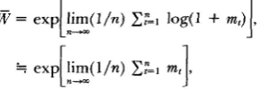
T h e geometric average of the population mean fitness is:

W

= Iim

(w,w,

. .

Wn)"n, ( 2 )

"'pi

which equals the long-term average rate of population growth. In the evolution of a parameter of the genetic system, such as recombination rate, the geometric average fitness (2) calculated for each parameter value often gives a measure for the rate of increase of the modifier genes controlling the parameter (LEVINS 1968; LEWONTIN and COHEN 1969; KARLIN and MCGREGOR 1974), and thereby tend to be maximized as evolutionary consequences although not always (GILLESPIE 198 l ) . In this paper, to con- centrate on the relation between the evolution of recombination rate and the way the environment fluctuates, we adopt the simplifying assumption: the recombination rate which maximizes the geometric average of population fitness ( 2 ) is the one to be attained through evolution.

T h e Malthusian parameter m, is the per capita rate of net population growth, and equals the fitness Wr minus 1 : m, =

W ,

-

1 , whose arithmetic average is related to W a s :

C:=l

Iog(1

+

m,)

1

,

r

1 ( 3 )

= exp

1.-

lim(l/n) CL1 m,

J

,

provided that m, is small. Therefore the long-term geometric average of the population fitness is related to the long-tErm arithmetic average of the Malthusian parameter by W =

exp(6).

From equation (I), the change of genotype frequency X , in a generation is

Xt"

-

X i = [ ( l

+

h,s,)/W, - 1 ] X :

-

rh,D,, ( 4 )

where we put S i = h,s,. If neither selection coefficient s, nor recombination rate r is very large, the difference equation

( 4 ) can be approximated by a differential equation:

dX,/dt = (h,s(t)

-

m)X, - h,rD, _{( 5 )}

with a continuous time parameter t, where i = 1 , 2 , 3 and

4 . Malthusian parameter is m = W - 1 =

E,

h,s(t)X,. Since continuous time dynamics are mathematically more tracta- ble than the corresponding discrete time dynamics, we begin our analysis with equation ( 5 ) instead of equation ( l ) , except for the case of extremely strong selection.

Another way to derive a continuous time model equation

( 5 ) is considering overlapping generation model (KIMURA,

1956).

By noting the relation

C,"=l

X, = 1 , we can rewrite equation (5) as a three-dimensional dynamical system of X = X I

+

X 4 , Y = XI

-

X 4 and 2 = X 2

-

X3:

dX/dt = 2s( t)X( 1

-

X )

-

2rD, dY/dt = [ s ( t ) - s(t)(2X

-

I ) ] Y , dZ/dt = [-s(t) - s ( t ) ( 2 X - l)]Z,

( 6 4

(6b)

( 6 4 where linkage disequilibrium is D = [2X - 1

-

Y 2

+

Z 2 ] / 4 .

T h e temporal average of s ( t ) is assumed to be zero. T h e long-term average Malthusian parameter f i of the population is

f i = Tlim(l/T) -

IT

s ( t ) [ 2 X ( t )

-

lldt. ₍₇₎

In the following, we examine the maximization of 6, the long term arithmetic average of the Malthusian parameter.

As shown in APPENDIX A, for any initial condition, both

Y ( t ) and Z ( t ) tend to zero as t increases, provided that the average Malthusian parameter f i is positive. In addition the positivity of 6 holds in the neighborhood of Y = 2 = 0. Hence, a closed invariant set ( ( X , Y , 2 ) ; 0 S X d 1 and

Y = 2 = 01 of the dynamics (6) is attracting (GUCKENHEIMER and HOLMES 1983). Moreover, the invariant set is globally attracting, as confirmed numerically in all the cases exam- ined in the following. After a transient period, the dynamical system (6) therefore is approximated by the one-dimensional system:

dX/dt = 2s(t)X(1 - X )

+

r(!h

-

X), ₍₈₎ and Y = Z = 0.

In the following, we study the optimal recombination rate rapt which maximizes the long-term average Malthusian parameter ( 7 ) , for various ways the selection coefficient s ( t )

fluctuates with time.

Linear analysis

If the magnitude of selection coefficient s( t ) is sufficiently smaller than the recombination rate r , equation (8) can be linearized around X = !h which is the equilibrium for s ( t ) =

0. T h e equation for the small deviation U ( t ) = X ( t )

-

$4 is:

dU/dt = s ( t ) / 2

-

rU, _{( 9 )} where w e neglect second order terms with respect to U ( t ) .

We first consider the simplest case in which s ( t ) is a sinusoidal function: s ( t ) = A cos(kt), where A and k are the amplitude and the frequency of the environmental fluctuations of selection coefficient. By integrating equation ( 9 )

and neglecting terms which damp out as t grows, we have the asymptotic solution of X( t ) and from this the long-term average Malthusian parameter (7):

A2r

2(r2

+

k2)' ( 1 0 )

(3)

0.0

+

0 10 _5o _T

2

1 -!-

100

Note that if a single predominant component of frequency

ko exists in the environmental fluctuation, the power spectrum density is approximated by: f (k) = (A2/2)6(k

-

ko),

where

a(.)

is the Dirac’s delta function, and equation ( 1 4 )

becomes equation (1 0) of the previous section.

Low pass filter effect

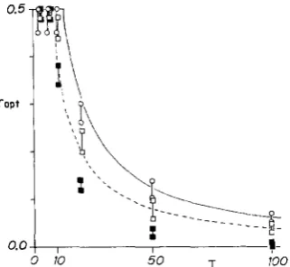
FIGURE 1 .-The optimal recombination rate ( rW) in an environment fluctuating with a single predominant period. Horizontal axis is the period T. The solid curve indicates the optimal recombination rate r,,, for weak selection calculated by equation (1 1); the broken curve, that for the strong selection limit given by equation (24). The bars show the intervals with which the evolutionarily stable recombination rate exists, obtained by computer simulation of recombination modifier dynamics (Table 2). Bars with open circles

(0), s = 0.05, linked modifier; bars with open squares (U), s = 0.5, linked modifier; and bars with closed squares @), s = 0.5, unlinked modifier.

Since equation (10) attains its maximum at r = k ,

the optimal recombination rate r,, which maximizes 6

under the constraint 0 5 r 5 Yz depends on the period To (= 2 s / k ) as:

-

{27r/T0,

if To Z 4?r,

Y2, if To 5 4s.

rapt

-

Thus, if the environment fluctuates slowly (large To), the optimal recombination rate is small, i.e., tight linkage is optimal, and is inversely proportional to the period To. On the other hand, in an environment fluctuating quickly (period To is shorter than 12.6 times average generation time), the optimal recombination rate is 0 . 5 , the maximum value, indicating no linkage between the loci.

Figure 1 illustrates the optimal recombination rate given by formula (1 1 ) together with the evolutionarily stable recombination rate obtained numerically by the genetic dynamics of a recombination modifier, which we will explain later.

Spectrum of environmental fluctuation

oidal fluctuations with different periods and amplitudes: More generally s ( t ) may be some superposition of sinus-

s ( t ) =

l-

[ A ( k ) sinkt

+

B(k) cosktldk, _{( 1 2 )}

where A(k) and B(k) are the weights for the fluctuation of period 27r/k. The power spectrum density (see, for example, NISBET and GURNEY 1982) of s ( t ) is defined by

f

( k ) = [A@)‘ + B(k)‘1/2, (1 3) which indicates the importance of the fluctuation component with period 2 s / k .

According to standard calculations, we can derive the asymptotic solution of the linearized system ( 9 ) and then the long-term average of Malthusian parameter from equations

(7), ( 1 2) and (1 3), and X = Yz

+

U, as

( 1 4 )

Equation ( 1 4) states that the long-term average Malthu- sian parameter 6 is the integral of the power spectrum density f ( k ) multiplied by a weighting factor r / ( r 2

+

k2).

The factor decreases monotonically with k and is very small for k much larger than r-it operates on f ( k ) as a “low pass filter” which selectively filters out high frequency components of the environmental fluctuation.

Therefore, if the fluctuation consists of several components of different frequencies, those of lower frequencies

(i.e., longer periods) have stronger effects on the population mean fitness, and hence on the optimal recombination rate. For example, Figure 2 illustrates the case in which the fluctuation has two components of frequencies k l and

k 2 ( k l

<

k2), such as the tidal and the annual periods. Since

the power spectrum is: f ( k ) = A%(k - R I )

+

B26(k

-

k z ) ,

the average Malthusian parameter is:

6 = A%/(?

+

k:)

+

B 2 r / ( r 2

+

k ; ) . _{( 1 5 )}

According to both numerical and analytical calculations, if A‘ and B 2 are of the same order of magnitude, i.e., the two components are comparable in strength, then the Mal- thusian parameter (1 5 ) is unimodal as a function of r , with the peak very close to k l (the smaller of the two frequencies), which is the optimal recombination rate under an environment fluctuating purely with the longer period component. The magnitude of the shorter period component must be far stronger for both components to be similarly influential to the optimal recombination rate in the face of low pass filter effect. Then +i is a bimodal function of r. Figure 2

illustrates a jump of the optimal recombination rate when the relative importance of two components changes gradually. The optimal recombination rate is exclusively regulated by the longer period component until its relative importance becomes as low as %25 of the shorter period component.

The low pass filter effect also explains why the optimal recombination rate for periodic s ( t ) is determined only by the basic period, and is insensitive to the “shape,” which is determined by harmonics of higher frequencies.

As to the optimal recombination rate for the general power spectrum pattern, we prove the following proposi- tions in Appendix B.

Proposition 1. The optimal recombination rate is between the

minimum and the maximum frequencies of environmental jluc-

tuation: kmin 5 rapt 5 k,,,.

Proposition 2. I f f ( k ) is a decreasing function of k, then + i ( r ) is a decreasing function of r, as f a r as linear analysis is appli- cable.

Many examples of random noise observed in nature have a decreasing power spectrum f ( k ) , including “l/f noise” and “pink noise” (NISBET and GURNEY 1982). Hence we may call them “noisy” fluctuations. For instance, the ower spec-

(>O) is the autocorrelation. From equation ( 1 4 ) , we have: trum of pink noise is f (k) = A 2 ( 2 / s ) a / ( a 2

+

k

?

), where a

+i = A 2 / ( a

+

r ) , _{( 1 6 )} which is, in fact, monotonically decreasing with r .

(4)

380

-28

,

I

+28

7

-28

,

I

A. Sasaki a n d

Y.

Iwasa

LO

iWR0

0.5

-

0.0- I 1 1 , I I 1 ,

-28

0 500 Kxx)

t

LO

R/RO

0.5-

0.0 1 , 1 , I , I I [

i i i / m O

C

r

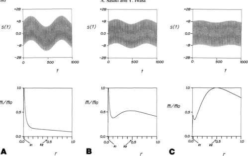
FIGURE 2.-Low pass filter effect. Upper figures illustrate selection coefficient s ( t ) fluctuating with time t having two strong components of different frequencies (kl = 0.01 and kz = 0.5). for various ratios of the relative importance of the components (A*/B* = I/5 in (A), '/qs in

(B), and %zs in (C)). Lower figures show the long-term average Malthusian parameter A (plotted as the ratio to the maximum value A.) versus recombination rate Y when s ( t ) fluctuates as shown in upper figures [calculated by equation (15)]. Even if the lower frequency component is much weaker than the higher frequency component, it is more influential in determining the optimal recombination rate (in (A) and (B)).

d u e to the low pass filter effect of the genetic dynamics. In (C), we further reduce the relative importance of the longer period component, and the Y~ which attains the peak Malthusian parameter A. jumps to the one corresponding to the higher frequency (shorter period) component.

valid only for Y sufficiently larger than t h e selection intensity

1s

I.

Therefore, Proposition 2 rather tells us that t h e optimal r is very small-at most of t h e same o r d e r of magnitude as

s ( t ) if t h e power spectrum is monotonically decreasing. These results suggest that not all kinds of environmental fluctuation make a large recombination rate advantageous; rather t h e fluctuation must have a significant periodic component. T h e following proposition confirms this conjecture:

Proposition 3. I f f ( k ) locally increasing at k = 0 so that: f ( R ) 2 f (0)

+

ck, (0 S k 5

a),

(17)

for some c > 0 and i

>

0 , then m ( r )

>

m(0) holds for suficiently small r

>

0 .

In contrast to noisy fluctuation with a decreasing power spectrum, a power spectrum f (R) increasing with k a r o u n d

k = 0 indicates some "orderly" structure of fluctuation, though its period may be blurred. T h e n , there exists a n optimal recombination rate which is positive, according t o Proposition 3.

Strong selection limit

If selection is not weak, t h e nonlinearity of the dynamics causes interaction between modes of different periods; thus t h e linear analysis in t h e last section fails.

H e r e we consider the o t h e r extreme, a strong selection limit, in which the selection coefficient s ( t ) = + I , indicating that genotypes under their unfavorable environment have

zero viability or null fertility. If selection is very strong, we can n o longer use the continuous time models such as equations (6) a n d (7). Instead we start with t h e discrete time model as follows.

Under t h e strong selection assumption, we have

X'I = X i , a n d X!, =

X i ,

for t

>

i,,, (18)

for any initial condition, where is t h e generation when t h e first environmental change occurs. T h i s is because all t h e genotypes in the ( i o

+

1)th generation are produced from recombination between t h e preexisting genotypes which themselves a r e doomed t o vanish in t h e new environment. T h i s is t h e extreme example of t h e general tendency that both Y ( t ) = X I

-

Xr

a n d Z ( t ) = X,

-

XJ

in equation (6) tend t o zero as t increases.

W e assume that, in each generation, natural selection a n d recombination occur in that order. Let XI = X :

+

X i ,

a n d let X, be the corresponding quantity after selection a n d before recombination. T h e n we have t h e recursion equations (for t

>

io):

XI

= ( 1

+

SI)Xl/W,, x,,, =

XI

+

r[l/p

-

rill

( 1 9 4

( 1 9b) where W, = 1

+

s,@X,

-

1). W e combine these two as:

x,+,

= r / 2

+

(1

-

r)(l

+

s,)xl/[l

+

s,(2x,

-

I)]. ( 2 0 )

(5)

the value oi st as: I I

(21)

regardless of the value of X,. Consequently, the population fitness in the ( t

+

1)th generation, Wt+l, is given by

It,;

r/2, if s, = 1, if st = -1, Xt+I =

(22)

{

:,

-

r , if st+l = st,

ifs,+l # st.

Wt+I = 1

+

St+1(2Xt+I

-

1) =

First w e consider a periodic environment, so that either

st = +1 or st = -1 holds during successive 7 generations,

i.e., the duration 7 is the number of generation during which st remains the same. T h e n the long-term average of the geometric mean fitness is

w

= exp lim(l/n)

c;=l

logw,]

L+-

(23)

[

I

= exp ( l / ~ ) l o g ( r )

+

(1

-

1/7)log(2

-

r )

.

By setting the derivative of (23) with respect to r be zero, we conclude that the optimal recombination rate r,, which maximizes (23) is inversely proportional to the duration 7 :

(24)

{2/7, i f 7 2 4,

!h, if 7 5 4,

rapt =

because of the constraint of r 5 !h. Noting that the duration

7 equals half the period, this formula gives a result numeri-

cally similar to the weak selection case (1 1) (see Figure l ) , but rapt is smaller in (24) than in (1 1).

T h e same analysis applies to a nonperiodic environment. Actually, the optimal recombination rate in the strong selection limit is determined only by the average number of environmental changes in the long time interval. For instance, in jump-type Markovian processes with transition rate

p

per generation:

P(St+l = f l 1st = T1) =

p,

₍₂₅₎

the optimal recombination rate is given by equation (24)

where 7 equals the relaxation time l/p; i.e., r , , = 2p.

A Markovian j u m p type process has a power spectrum density which monotonically decreases with the frequency, because it is the discrete time version of pink noise. For weak selection fluctuating with such a power spectrum, the optimal recombination rate must be small, as shown by Proposition 2 of the previous section. However, in the strong selection limit, r,,, may be large when the relaxation time is sufficiently short. T h e optimal recombination rate under “noisy” fluctuations therefore depends greatly on the selection intensity. This result contrasts with the case of periodic fluctuations in which the optimal recombination rate is similar between the two extremes of selection intensity: weak and strong selection limits.

Two-state Markovian jump selection

If natural selection is mildly strong, neither analysis developed in the last two sections is applicable. Here we examine a particular class of environmental fluctuations for which the optimal recombination rate can be analytically derived for wide range of selection intensity.

We assume that the selection coefficient ( s ( t ) ;

-

0

<

t < 031 is a “two-valued stationary Markov process,” i.e., s ( t ) takes

one of the two distinct values f s , and randomly jumps between them with a transition rate

p:

P(s(t

+

A t ) = T s l s ( t ) = +s) = pAt

+

o(At). (26)

P / s

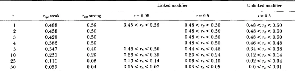
FIGURE 3.-Optimal recombination rate when the selection coefficient jumps between f s with transition rate

p .

The long-term average Malthusian parameters 6 is calculated by numerical integration of equation (28), for various values of the parameters. The optimal recombination rate rapt is obtained for each pair of parameters p and s fixed. This figure illustrates the relationship between

r0,,/sandp/s(0,s=0.01;0,s=0.1,A,s=0.5,and0,s= 1.0).

Data points are on a single curve irrespective of the magnitude of

s. The solid curve represents the harmonic mean formula (29b); the broken line, the geometric mean formula (29a).

where A t is small. Since the rate of state change is p, the autocorrelation of s ( t ) decays as exp(-pt). T h e inverse 1/p is the relaxation time; the average duration of each environment. T h e stochastic process {X( t); 0 5 t

<

m] is then defined as the solution of a stochastic differential equation (8). Although {X(t); 0 S t < m] by itself is non-Markovian, the vector-valued stochastic process ((X(t), s ( t ) ) ; 0 d t

<

01

is Markovian.

This process is mathematically equivalent to the one locus two allele model with mutation and stochastic selection analyzed by MATSUDA and ISHII (1 98 1) if we replace mutation by recombination. T h e exact solution for the stationary joint distribution of X and s is known [equation (3.7) in

MATSUDA and ISHII 198 11 as:

c,

(A

-

X)(X

-

b )

‘

/IF-cl.

(27) +(X, fs) =

{

o , [ ( x - a ) ( B - x ) for b

<

1

X

<

A ,

for 0

<

X

<

b, A

<

X

<

1, where F,(X) = +2sX(1

-

X)

+

r(Yz

-

X); A and a are the two roots of quadratic equation F+(X) = 0; B and 6, those of F-(X) = 0; Q = p / J 4 s n

+

r 2 ; and C, a normalizing factor. T h e mean Malthusian parameter (7) of the population is

@(X)dX, (28) r(2X

-

1)2

e = $

2X(1 - X) where @(X) = d(X, +s)

+

4(X, -s).

Given the parameters s (selection intensity) and

p

(transition rate of environment), the Malthusian parameter f i is calculated by numerical integration of equation (28) for various values of r , and the optimal recombination rate r,,, is obtained as a function of s and

p.

Figure 3 illustrates the results. If w e change the time unit for the above system, the three rate parameters, rapt, s, and

p ,

are multiplied by the same factor. Since any relationship among rapt,

p

and s must remain valid under such an alteration, the ratio ropt/s must be a function of pis, independent of the absolute values of

(6)

382 A. Sasaki and Y . Iwasa

TABLE 2

Evolutionarily stable recombination rate for periodical fluctuation

Linked modifier

~ _ _

Unlinked modifier

7

1 2 3 4 5 10 25 50

r,, weak 0.488 0.458 0.420 0.382 0.347 0.231 0.1 1 1 0.059

r,, strong s = 0.05 s = 0.5

0.50 0.50 0.50 0.50 0.40 0.20 0.08 0.04

0.45 r E < 0.50 0.48 < r E < 0.50

0.48 < rE < 0.50

0.48 < rs < 0.50

0.20 < rE < 0.24 0.48 < r E < 0.50

0.44 < r E < 0.48

0.06 < T E < 0.10

0.03 < r E < 0.05

~~

s = 0.5 0.48 < TE < 0.50

0.48 < r E < 0.50

0.48 < T E C 0.50 0.46 < r E < 0.48

0.34 < T E < 0.38

0.12 < rE < 0.14 0.02 < rE < 0.04 0.0 < T E < 0.01

~~~

7: duration of each environment (half period); s: selection intensity; r,,,: the optimal recombination rate given by equation (1 1) for weak

selection limit and equation (24) for strong selection limit. T h e interval including the evolutionarily stable recombination rate is given both for linked (r0 = 0) aid unlinked(ro = 0.5)modifiers.

larger than 1 : but for small p / s , it is approximately half of the geometric mean of s and

p :

p

s,

-

\o.5(2sp/(s

+

P)),

p

> s. (29b) Given the transition rate

p ,

the optimal recombination rate monotonically increases with the selection intensity s.

In the limit of weak selection, equation (29b) states that the optimal recombination rate is as small as the selection intensity s, as suggested by Proposition 2.

When p / s is smaller than 0.01, numerical integration of (28) is technically very difficult. K. ISHII (personal commu- nication) observed that, for p / s as small as r,,, becomes proportional to

p .

Numerical analysis of modifier dynamics

In the foregoing analysis, we have assumed that the recombination rate which maximizes the long-term geometric average of the population fitness (rapt) is the one to be evolved. In this section, we numerically examine the genetic dynamics of a recombination modifier to determine whether o r not the optimal recombination rate can be obtained as an evolutionary consequence of modifier dynamics, and to check the predicted dependence of the evolutionarily stable recombination rate on the temporal structure of environmental fluctuation.

Consider an additional locus M with two alleles m l and m2, controlling the recombination rate between two selected loci A and B. T h e recombination rate is determined by the diploid genotype: genotypes mlml, mlm2 and m2m2 realize the recombination rate r l , ( r l

+

r2)/2 and r2, respectively. T h e loci A , B and M are linearly arranged on the map in this order, and the recombination rate between modifier M

and locus B is ro. We then examine which of the modifier alleles will spread for various temporal structures of the environmental fluctuation.

For most cases, there exists a unique evolutionarily stable recombination rate TE: if r l and r2 are both larger o r both

smaller than T E , after many (about l o 3 to lo5) generations,

the allele giving the recombination rate closer to ?-E becomes

quasifixed (its frequency becomes larger than 99%). If instead rE is between r I and r2, the polymorphism of two alleles

is stably maintained. Hence we expect that after repeated events of invasion and replacement of various modifier alleles, the recombination rate between A and B would evolve toward rE.

In some cases, however, the system shows bistability: there

are two recombination rates both of which are evolutionarily stable against alleles showing slightly different recombination rates.

Tables 2 to 4 show the interval that includes the evolutionarily stable recombination rate YE (estimated by simula-

tions of genetic dynamics, see APPENDIX c for details) and the optimal recombination rate ropt (derived theoretically in the preceding sections).

Fluctuation with a single period

T h e results for the case of periodically fluctuating selection are listed in Table 2 and illustrated in Figure 1 . T h e evolutionarily stable recombination rate Y E is accurately

predicted by the optimal recombination rate rapt given by equation ( 1 1) for the weak selection limit and by equation (24) for the strong selection limit in Table 2. T h e rE monotonically decreases with the period of environmental fluctuation. It is relatively insensitive to the magnitude of the selection coefficient: rE is similar for s = 0.5 and s = 0.05, but Y E for strong selection tends to be smaller than that for

weak selection, as predicted by rapt. T h e rE is also insensitive to the linkage between the modifier and the selected loci: it is similar for completely linked (YO = 0) and unlinked ( r o = 1/2) modifiers, though the latter tends to be smaller.

This case is the same as the genic modifier model studied

by CHARLESWORTH (1 976) except that he assumed diploid

genetics with marginal overdominance at both selected loci.

CHARLESWORTH reported that rE was small both for very

short periods of fluctuation and for very long periods, and is the highest for an intermediate period. This conclusion is different from ours and can be explained by that he calculated modifier evolution only for several hundred generations-we numerically followed his genic modifier model of diploid systems much longer (about 1 O4 generations) and obtained the monotonic decrease of rE with the environmental period.

Fluctuation with two strong components

Table 3 shows the results for the case in which the fluctuation of the selection coefficient is the superposition of two periodic components. If the two components are comparable in strength, the evolutionarily stable recombination rate is very close to the optimal one for the fluctuation only with the longer period component; hence the low pass filter effect works in modifier genetic dynamics. If the relative importance of the long-period component decreases as low as ( A 2 / B 2 = ) I/z5 of the short-period one, the system

(7)

In short, all the important features of the evolutionarily stable recombination rate in fluctuating environments, predicted theoretically by the optimization model, are thus confirmed by the evolutionary dynamics of a recombination modifier.

TABLE 3

Low pass filter effect

A B

0.1 0.0 0.006 < rE < 0.008

0.1 0.1 0.006 < YE < 0.008 0.05 0.1 0.006 < YE < 0.008 0.02

0.005 0.1 0.35 < r E < 0.45

0.0 0.1 0.38 < r E < 0.42

0.1 0.006 < YE) < 0.01, 0.34 < r E 2 < 0.38"

Evolutionary stable recombination rate for the case when the selection coefficient is a superposition fluctuating with two components: s ( t ) = A sin (0.01t)

+

E sin (0.5t). The long-term average Malthusian parameter is shown in Figure 2.

a The domain of attraction for rE,: 0.0 5 r < 0.1; that for rE2:

0.1 < r 5 0.5.

respect to the invasion of a modifier, showing a slightly different recombination rate. As A2/B2 decreases further, the equilibrium with the lower recombination rate disap- pears and the one with the higher recombination rate becomes globally stable. Thus the jump of the evolutionarily stable recombination rate, predicted by the corresponding optimization model (Fig. 2), is demonstrated by the modifier genetic dynamics (Table 3).

Noisy fluctuation

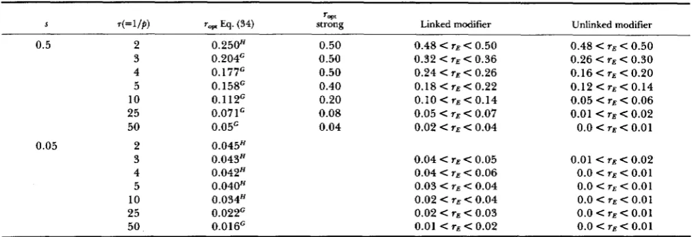
Table 4 illustrates the results for the case in which the selection coefficient fluctuates with pink noise, realized by Markovian jump processes. Again the ?-E can be approxi-

mated by equation (29) for the optimal recombination rate. The evolutionarily stable recombination rate is small for weak selection and increases with the magnitude of the selection coefficient. The contrast between sensitive dependence of rE on the selection intensity for noisy fluctuation and insensitive dependence for orderly fluctuation is thus confirmed.

For pink noise fluctuation, we observe that the strength of linkage between the modifier

M

and the selected locus B

does not affect ?+E much, but ?-E tends to be smaller for

unlinked modifiers (ro = %) than for tightly linked ones

(ro = 0) especially when r,,,

<

0.05.

DISCUSSION

For the simplest models of evolution in a temporally changing environment, life history traits which maximize the geometric average population fitness are the ones to be evolved (LEVINS 1968; LEWONTIN and

COHEN 1969). With sophisticated analysis, KARLIN

and MCGRECOR (1 974) demonstrated that the evolu-

tionary consequences of modifier gene dynamics often maximize the geometric average of the population fitness, but not always

(e.g.,

GILLESPIE 1981 for mutation modifier).

According to our numerical analysis, the optimization model works very well in predicting how the evolutionarily stable recombination rate depends on the temporal structure of environmental fluctuation-all the predictions derived from the optimization model also hold for the evolution of modifier dynamics.

CHARLESWORTH (1 976) claimed that significant ev-

olution

of

a high recombination rate requires strong linkage between the modifier and one of the selected loci, and hence considered it as demonstrating a limi- tation of the optimization approach. However, our computer similation shows that, although the evolution rate

is

slower for unlinked modifiers than for linked ones, the evolutionarily stable recombination rate ?-E for unlinked modifiers can be high: it is close

to the maximum value

(0.5)

for cyclic fluctuation with a short period (T = 1

-

4);

hence it is not very different from Y E for linked modifiers, both for our haploid

TABLE 4

Evolutionarily stable recombination rate for fluctuation with Markovian jump model

y,,

S .(=I/$) r v Eq. (34) strong Linked modifier Unlinked modifier

0.5 2

3 4 5 10 25 50

0.05 2

3 4 5 10 25 50

0.250H 0.204' 0.177' 0.158' 0.112G 0.071' 0.05'

0.045H 0.043H 0.042H 0.040" 0.034" 0.022G 0.016'

0.50 0.48 < r E < 0.50

0.50 0.32 < YE < 0.36

0.50 0.24 < r E < 0.26

0.40 0.18 < r E < 0.22

0.20 0.10 < rE < 0.14 0.08 0.05 < r.5 < 0.07 0.04 0.02 < rE < 0.04

0.04 < YE < 0.05 0.04 < r E < 0.06

0.03 < r E < 0.04

0.02 < < 0.04 0.02 < r E < 0.03

0.01 < rE < 0.02

0.48 < < 0.50 0.26 < rE < 0.30 0.16 < rE < 0.20 0.12 < rE < 0.14 0.05 < r E < 0.06

0.01 < r E < 0.02 0.0 < r E < 0.01

0.01 < r E < 0.02 0.0 < < 0.01

0.0 < 71 < 0.01

0.0 e r E < 0.01

0.0 < Y E < 0.01

s: selection intensity; 7 = 1/p: relaxation time; rw: optimal recombination rate calculated by equation (29a) (geometric mean formula,

(8)

384 A. Sasaki and Y. Iwasa

model (Table

2)

and for CHARLESWORTH’S diploid overdominance model. T h e ?-E tends to be smaller for

unlinked modifiers than for linked ones: the difference becomes significant when the optimization model predicts a small recombination rate

(r,,,

<

0.05), both for periodic and noisy fluctuations (Tables

2

and 4). Hence, the concept of the optimal recombination level for a given environment works better than CHARLES-

WORTH (1 976) concluded.

T h e main simplifying assumption adopted in this paper is the special way the fitnesses of the four genotypes correlate (Table 1). Since the average fitnesses of the two segregating alleles are exactly the same for both loci, the polymorphisms at both loci are stably maintained, as proved in APPENDIX A. But the result of our analysis should be of no biological importance if a slight fitness difference between alleles could break the genetic polymorphism, which is necessary for the advantage of recombination to manifest itself.

Fortunately, we can prove (see APPENDIX A) that a protected polymorphism is structurally stable for the deterministic fluctuation of s(t) with a positive recombination rate-polymorphisms at both loci should be maintained for any perturbation of sufficiently small magnitude. Intuitively speaking, this is because recombination, associated with the temporal fluctuation of epistasis, contributes genetic variation by producing two currently nonfit genotypes with equal frequencies, and thus reduces the unbalance between allele frequencies. T h e numerical analysis of the dynamics (1) with small perturbations, explained in APPENDIX A , supports the stabilizing effect of recombination, and further suggests that the effect is strongest for an intermediate r which produces a sufficiently positive advantage measured by f i .

Therefore, in a haploid two-locus model of changing environment, a polymorphism can be structurally stable: this makes a sharp contrast with the one-locus haploid model, in which neither random nor system- atic fluctuations of selection coefficient can make a polymorphism structurally stable-quasifixation is certain if there is no mutation (KIMURA, 1954; GIL-

However, the above mechanism for polymorphism is not effective if the fitness difference between alleles is large. Then the polymorphism needs to be maintained by additional processes, such as mutation-selection balance, frequency dependent selection, or het- erotic interaction in diploid genotypes. We may examine the optimal recombination rate in these more general systems in which we consider processes re- sponsible for polymorphism. The advantage of recombination may possibly have a similar relation with the temporal structure of environmental fluctuation

(e.g.,

the power spectrum of selection) to what the present LESPIE, 1973).

model concludes. For example, CHARLESWORTH’S

(1 976) recombination modifier model with marginal overdominance, which helps maintain the genetic variation, shows very similar results to the haploid model we studied, according to our numerical analysis.

Another shortcoming of our model is the assumption of a two-locus genetic system, instead of a polygenic system with many loci controlled by also many recombination modifiers. SLATKIN and LANDE’S (1976) model for the evolution of niche width under changing environment seems to have some analogy to the polygenic model of the evolution of recombination, if we assume that a larger within-family variance of traits is produced by a higher recombination rate.

In spite of these potential problem with the under- lying genetic system, our analysis has its value in revealing new aspects of the evolution of recombination rates under various ways the environment fluctuates. The results are summarized as:

First, if the environment fluctuates periodically, the optimal recombination rate is approximately inversely proportional to the period, both in weak and strong selection limits. We expect that this result holds also

for selection

of

intermediate intensity, and conjecture that the optimal recombination rate is relatively insensitive to the magnitude of selection in the orderZy (or approximately periodic) fluctuation of the environment. The average Malthusian parameter rii for the model equation (8), in which s ( t ) alternates between s and -s with the duration 7 for each value, is obtained

by equation (3.6) of ISHII, MATSUDA and OCITA ( 1 982, p. 341) with the necessary replacement of parameters. T h e numerical calculation of their result supports an insensitive dependence of the evolutionarily stable recombination rate on the selection intensity s.

Note that the period in the model is measured by the number of generations. Therefore, if we compare several organisms having different generation times growing under the same periodic environment, the optimal recombination (per generation) rate should increase with the generation time. According to (1 l ) , if the generation time is as long as a tenth of the environmental period, ropt is the maximum value 0.5, which is realized when the two loci are located on different chromosomes or far apart on the same chro- mosome.

(9)

Optimal Recombination

creasing function of the frequency. T h e optimal recombination rate for periodic fluctuation is determined only by the basic period irrespective of the shape of fluctuation which is given by harmonics of high frequency. In a similar vein, temporal fluctuation with a period shorter than the generation time of organisms has negligible effect on the optimal recombination rate because of the averaging.

If the environment has two dominant components of fluctuation (for example, tidal and annual periods), and if the one with shorter period is so strong that even after the filtering by the demographic dynamics the strength of the two components are comparable, then the optimal recombination rate may discontin- uously change at some point as the relative strength of the t w o components changes continuously. This suggests a possible dichotomy of genetic systems

dif-

fering in the fraction of sexual reproduction when life history parameters gradually change.

Third, if the environmental fluctuation is noisy,

showing a decreasing power spectrum pattern, the optimal recombination increases with the selection intensity. Specifically in pink noise, r,,, is close to one half of the harmonic average of the selection intensity (s) and the environmental transition rate

(p),

when

p

>

s and is half of their geometric average when

p

C s. In the noisy processes, the duration of each environment has a large variance so that there are many short runs of the same environment as well as long ones. When selection is weak, the genetic dynamics slowly track environmental shifts, not responding to short runs; hence very long runs of the same environment that occasionally appear make a high recombination rate disadvantageous. However, as the selection intensity increases, the system becomes able to respond to shorter runs of each environment; hence the optimal recombination becomes larger, until finally both short and long runs are equally important in determining the optimal recombination, so that the average environmental duration decides the optimal value, as in the strong selection limit.

T h e evolutionary advantage of recombination has been previously discussed in the context of the benefit of sexual reproduction. Possible factors favoring sexual reproduction in the face of meiotic cost

(MAYNARD

SMITH

1978)

include (1) acceleration of the accumulation rate of favorable mutant genes by combining separately created ones into the same genome (FISHER

1930; CROW and KIMURA 1965; MAYNARD SMITH 197 1 ; FEUENSTEIN 1974; FELSENSTEIN and YoKO- YAMA 1976; STROBECK, MAYNARD SMITH and CHARLESWORTH 1 9 7 6 ) ,

(2)

protecting a population from irreversible accumulation of deleterious muta- tions (MULLER 1964; HAIGH 1 9 7 8 ) , (3) frequency dependent selection favoring rare types caused either by intraspecific competition or via host-parasite and

predator-prey interactions

(WILLIAMS

and

MITTON

1973; LEVIN

1975; MAYNARD

SMITH

1976; HAMIL-

TON

1980),

and

(4)

the switching over of genotypes in

temporal or spatial fluctuations of environment (SLAT-

CHARLESWORTH and STROBECK

1977; HAMILTON,

HENDERSON

and

MORAN 198

1). In this paper we have

developed the last hypothesis.

T h e model we studied in this paper is based on only one of several hypotheses on the evolutionary advantage of recombination, which are equally plausible at the present stage. After detailed examination of each possible mechanism, as we did in the paper, we will then be at a stage to evaluate the relative importance of different mechanisms for the evolutionary advantage of recombination, and will be able to answer why sexual reproduction is so prevalent in nature.

We sincerely thank Professor HIROTSUCU MATSUDA, Kyushu University, for his encouragement throughout this study. We also thank BRIAN CHARLESWORTH, DAN COHEN, JOHN GILLESPIE, WIL-

LIAM D. HAMILTON, MASARU IIZUKA, KAZUSHIGE ISHII, SHIN-ICHI KUSAKABE, HIROYUKI MATSUDA, TERUMI MUKAI, NAOYUKI TAKA-

HATA and NORIO YAMAMURA for their helpful comments. This work was supported in part by a Grant-in-Aid for Special Project Research of Optimal Strategy and Social Structure of Organisms from the Japan Ministry of Education, Science and Culture.

KIN

1975;

CHARLESWORTH 1976; CHARLESWORTH,

LITERATURE CITED

CHARLESWORTH, B., 1976 Recombination modification in a fluctuating environment. Genetics 83: 181-195.

CHARLESWORTH, D., B. CHARLESWORTH and C. STROBECK, 1977 Effects of selfing on selection for recombination. Ge- netics 8 6 213-226.

CROW, J. F. and M. KIMURA, 1965 Evolution in sexual and asexual populations. Am. Nat. 9 9 439-450.

FELSENSTEIN, J., 1974 The evolutionary advantage of recombination. Genetics 7 8 737-756.

FEUENSTEIN, J. and S. YOKOYAMA, 1976 The evolution of recombination. 11. Individual selection for recombination. Genetics

FISHER, R. A., 1930 The Genetical Theory of Natural Selection. Oxford University Press, New York.

GILLESPIE, J. H., 1973 Natural selection with varying selection coefficient-a haploid model. Genet. Res. 21: 115-120. GILLESPIE, J. H., 1981 Mutation modification in a random envi-

ronment. Evolution 35: 468-476.

GUCKENHEIMER, J. and P. HOLMES, 1983 Nonlinear Oscillations, Dynamical Systems, and Bifurcations of Vector Fields. Springer, New York.

The accumulation of deleterious genes in a population-Muller’s ratchet. Theor. Popul. Biol. 14: 251- 267.

HAMILTON, W. D., 1980 Sex versus non-sex versus parasite. Oikos

HAMILTON, W. D., P. A. HENDERSON and N. A. MORAN, 198 1 Fluctuation of environment and coevolved antagonist polymorphism as factors in the maintenance of sex. pp. 363- 381. In: Natural Selection and Social Behavior, Edited by R. D. ALEXANDER and D. W. TINKLE. Chiron, New York.

ISHII, K., H. MATSUDA and N. OGITA, 1982 A mathematical model of biological evolution. J. Math. Biol. 1 4 327-353. KARLIN, S., and J. MCGREGOR, 1974 Towards a theory of the

evolution of modifier genes. Theor. Popul. Biol. 5 59-103.

83: 845-859.

HAICH, J., 1978

(10)

386 A. Sasaki a n d Y. Iwasa

KIMURA, M. 1954 Process leading to quasi-fixation of genes in natural populations due to random fluctuations of selection intensities. Genetics 39: 280-295.

KIMURA, M. 1956 A model of a genetic system which leads to closer linkage by natural selection. Evolution 1 0 278-287. LEVIN, D. A., 1975 Pest pressure and recombination systems in

plants. Am. Nat. 109 437-45 1 .

LEVINS, R., 1968 Evolution in Changing Environments. Princeton University Press, Princeton, New Jersey.

LEWONTIN, R. C. and D. COHEN, 1969 On population growth in a randomly varying environment. Proc. Natl. Acad. Sci. USA 62: 1056-1060.

Stationary gene frequency distribution in the environment fluctuating between two distinct states. J. Math. Biol. 11: 119-141.

MAYNARD SMITH, J., 1968 Evolution in sexual and asexual populations. Am. Nat. 102: 469-473.

MAYNARD SMITH, J., 1971 What use is sex? J. Theor. Biol. 3 0

MAYNARD SMITH, J., 1976 A short term advantage of sex and recombination through sib-competition. J. Theor. Biol. 63:

MAYNARD SMITH, J., 1978 The Evolution o f s e x . Cambridge Uni- versity Press, New York.

MULLER, H. J., 1964 The relation of recombination to mutational advance. Mutat. Res. 1: 2-9.

NISBET, R. M. and W. S. C. GURNEY, 1982 Modeling Fluctuating Populations. John Wiley & Sons, New York.

SLATKIN, M., 1975 Gene flow and selection in a two-locus system. Genetics 81: 787-802.

SLATKIN, M. and R. LANDE, 1976 Niche width in a fluctuating environment-density independent model. Am. Nat. 110: 31-

55.

STROBECK, C., J. MAYNARD SMITH and B. CHARLESWORTH, 1976 The effects of hitch-hiking on a gene for recombination. Genetics 82: 547-558.

The interrelations of inversions, heterosis and recombination. Am. Nat. 72: 447- 452.

Niche overlap and invasion of competitors in random environments. I. Models without demographic sto- chasticity. Theor. Pop. Biol. 20: 1-56.

Why reproduce sexually? J. Theor. Biol. 3 9 545-554.

Communicating editor: B. S. WEIR MATSUDA, H. and K. ISHII, 1981

319-335.

245-258.

STURTEVANT, A. H., and K. MATHER, 1938

TURELLI, M. 198 1

WILLIAMS, G. C. and J. B. MITTON, 1973

APPENDIX A

In the following, we first prove that the 3-dimensional dynamics (6) are effectively described by the I-dimensional dynamics (8), and then we show that a protected polymorphism is structurally stable.

Lemma 1. Both variables Y ( t ) and Z ( t ) in equations (6) tend to

zero for any initial condition, provided that the long-term average of the Malthusian parameter (7) is positive.

Proof. Equation (6b) can be rewritten as

dY/dt = k(t)Y, ( A l l where k ( t ) = s ( t )

-

s ( t ) [ 2 X ( t ) - 11. According to (7), when the average of s ( t ) is zero, we have limT, (1/T) k ( t ) d t = -6.

For an arbitrary small positive number 6 > 0 , we have

I

Y ( t )

I

Y(0)

I

exp(-(6

-

6 ) t ) (-42) for sufficiently large t. Hence if 6 is positive, Y ( t ) exponentially converges to zero as t grows infinitely large. Similarly, from (6c), we can derive that Z( t) goes to zero as t grows. Here, -6

is called the “Lyapunov exponents” of variables Y ( t ) and Z ( t ) ; which govern their asymptotic behavior as Y ( T )

-

exp(-iT) and Z( T)

-

exp(-fiT). T h e positivity of 6, therefore, implies that both Y ( t ) and Z ( t ) exponentially decrease with the asymptotic rate 6 as t increases for any initial condition. Thus we proved Lemma 1.

Lemma 2. Long-term average Malthusian parameter 6 is positive in the neighborhood of Y = Z = 0.

ProoJ: First, we note that Y ( t ) = Z ( t ) = 0 holds for all t if we start with the initial condition Y(0) = Z(0) = 0. Therefore

{ ( X , Y, 2); 0 5 X 5 1, Y = Z = 01 is an invariant set of the dynamics (6). Now we examine whether the invariant set is attracting or not. Since D in

(sa)

depends on Y and Z only through second order terms, we can neglect them in the neighborhood of Y = 2 = 0. Letting U = X

-

%, the system then becomes

dU/dt = 2 s ( t ) [ %

-

U’]

-

rU, _(‘43)

together with equation (AI) for Y and a similar one for Z. Using (A3), the integrand of equation (7) is

where g ( U ) = !h

-

U‘ is positive because

I

U1 < % from defi- nition. Then equation (7), the long-term average of the Malthu- sian parameter, is

Since the first term of (A5) vanishes, we conclude 6 > O.

Combining Lemma 2 with Lemma 1, we conclude that Y ( t )

and Z ( t ) converge to zero in the neighborhood of Y = Z = 0, i.e., the line segment ((X, Y, Z); 0 5 X 5 0 , Y = Z = 01 is a locally attracting invariant set (GUCKENHEIMER and HOLMES, 1983). Therefore, the dynamical system is effectively described by the one-dimensional equation (8) if both Y = X I

-

X4 and Z =

X,

-

X s are sufficiently small initially.

We numerically confirmed 6 > 0 holds for any initial condition, and that the invariant set is in fact globally attracting-

Y and Z converge to zero with time and the system becomes one-dimensional. T h e same tendency is emphasized in the strong selection limit, in which X I = X4 and X, = X 3 hold for all the generations after the first environmental change.

Given that Y ( t ) and Z ( t ) coverge to zero, we prove that the polymorphism is protected at both loci as follows: Let us consider the reduced dynamics (8) in the neighborhoods of X = 0

and X = I , as:

d X / d t = r / 2 , X = 0 , (A6a)

dX/dt = -r/2, _X

+

1 (A6b)

where small terms (of higher order with respect to X and (1

-

X), respectively) are neglected. We can conclude from (A6) that X ( t ) must stay away from boundaries; i.e., there exists a positive constant 6 > 0 so that 6 < X ( t ) < 1 - 6. Together with

Y ( t ) = Z ( t ) = 0, we conclude that the frequency of any genotype remains positive: X j ( t ) > 6/2 ( i = 1, 2 , 3 and 4).

Intuitive justification of the logic supporting the joint polymorphism is as follows: the relation Y = Z = 0 indicates X I = X, and X , = X 3 . Suppose that either pair of genotypes (say AB