Apparent negative interference due to variation in recombination frequencies.

(1)

Copyright 0 1989 by the Genetics Society of America

Apparent Negative Interference Due to Variation in Recombination

Frequencies

Torbjorn

Sall*

and Bengt 0. Bengtssont

*Department of Crop Genetics and Breeding, Swedish University of Agricultural Sciences, Svalov, Sweden, and ?Department of Genetics, Lund University, Lund, Sweden

Manuscript received December 8, 1988 Accepted for publication April 15, 1989

ABSTRACT

Variation in recombination frequencies may lead to a bias in the estimated interference value in a linkage experiment. Depending on the pattern of variation, the bias may be toward negative interference or toward positive interference, even when there is positive interference at the cytological

level. In this paper we have mainly concentrated on the case of negative interference. We use models to quantify this effect when data are derived from a backcross experiment or from the selfing of F1

individuals. The effect is quantitatively similar in the t w o cases. There is an upper limit to the size the

bias may reach for every given level of recombination. T w o reported cases of negative interference

in Drosophila and cultivated barley fall within this possible parameter range, i.e., the observed negative interference values could-at least in principle-be due solely to a variation in the recombination

frequencies in the experiments.

A

fundamental problem in the study of genetic linkage is the degree of dependence between recombination events in adjacent chromosome segments. This dependence is usually measured by the coefficient of coincidence, c, defined by

c = (the observed number of double crossovers)/(the number of double crossovers expected if crossing over occurs independently in the two segments).

T h e dependence is often expressed in terms of the interference I, which is defined by

I

= 1

-

c.

In eukaryotes the coefficient of coincidence is usually less than one (positive interference) for closely linked markers, and increases towards one for markers further apart (BAILEY 196 1). In bacteriophage, on the other hand, the coefficient of coincidence is usually larger than one (negative interference; STAHL

1969). It is customary to distinguish between two different types of negative interference, “high negative interference” and “low negative interference.”

High negative interference, also referred to as “localized negative interference,” occurs only for very closely linked markers and decreases with increasing recombination frequencies. Such high negative interference has been described for several bacteriophage (STREISINGER and FRANKLIN 1956; CHASE and DOER- MAN 1958; AMATI and MESELSON 1964), but was first observed in a eukaryote, the fungus Aspergillus nidu- lans (PRICHARD 1955). T h e effect may have several causes but the phenomenon is normally considered to

The publication costs of this article were partly defrayed by the payment of page charges. This article must therefore be hereby marked “advertisement” in accordance with 18 U.S.C. $1734 solely to indicate this fact.

Genetics 122: 935-942 (August, 1989)

be due to gene conversion at one of the centrally located markers (STAHL 1969).

The other type of negative interference found in phages, “low negative interference,” is independent of the distance between the markers and takes a constant value given the type of phage and the exper- imental conditions. This type of negative interference can be explained by heterogeneity among the individual virus chromosomes with respect to their recombin- ing opportunities (VISCONTI and DELBRUCK 1953). Thus, the effect arises because the descendant viral chromosomes are heterogeneous with respect to the recombination processes under which they were formed. Some of the virus particles stem from parents that never mated, whereas others originate from parents that mated and recombined several times.

Instances of negative interference are rare in ani- mals and plants, but the phenomenon has been observed, for example in Drosophila (MORGAN, STUR- TEVANT and BRIDGES 1925; GREEN 1975) and barley (Hordeum vulgare) (SBGAARD 1977; LARSSON 1985; T. SALL and B. 0. BENGTSSON, preliminary results). These results have normally been interpreted as being due to conversion of the central marker with no associated crossover [see, e.g., GREEN (1 975) and VON WETTSTEIN, RASMUSSEN and HOLM (1984)], but a detailed analysis of the phenomenon has not been made.

(2)

even when there is no “true” interference at the cytological level. Some simple models are used to investigate how much negative interference may be produced by this effect alone; in particular we deter- mine the maximum value of negative interference that can follow from the variance effect as a function of the estimated recombination values. We have also tried to assess whether this effect can be the cause of some of the reported cases of negative interference in Drosophila and Hordeum.

MODELS

Basic assumptions and definitions: We base our study on the observation of gametes produced by a set of individuals heterozygous for three linked loci

( A , B , C ) . The gametes can be grouped into four classes, i.e.

1 . gametes produced with no recombination = paren-

2. gametes produced with recombination between

3 . gametes produced with recombination between

4. gametes produced with recombination in both seg- tal type gametes

locus A and B only

locus B and C only

ments A-B and B-C.

Let the recombination frequency in segment A-B be

T A B and in segment B-C be T B C . If the coincidence

between the two segments is c , then the frequencies of the four types of gametes in the gametic pool are

1 . 1

-

TAB

-

r B [ ;

+

C r A B r B [ ;

2. TAB( 1

-

C r B C )

3 . rBC( 1

-

C T A B )

4. C r A B r B C .

Consider now the case where linkage is studied through a backcross to the triple recessive parent. Let

x 1 be the proportion of offspring with a parental phenotype, corresponding to the transmission of type

1 gametes, let x2 be the proportion of offspring cor-

responding to type

2

gametes, and let x3 and x4 be defined similarly. Note that in a backcross of this type the phenotype of an offspring describes exactly the genotype of the transmitted gamete (haplotype) from the heterozygous parent.

Given such a set of observations the standard way to estimate the values T A B , rBc and c is to use the

estimators R A B , R B c and C , defined by

R A B =

+

x4 ( 1 )

R E ( ; = x3

+

x4 (2)

C = x4 _{( 3 )}

(x2

+

x4)

(see any standard textbook in genetics, e.g., SUZUKI,

GRIFFITH and LEWONTIN 1981). It can be shown that all three expressions are maximum likelihood esti-

C r A B r B C

-

c ,

~ A B ~ B C

where A s E ( C ) is the asymptotic expectation. This means that the expectation of C is close to its desired value for large sample sizes. In order to obtain information about the relation between the size of the sample and the magnitude of the bias, computer sim- ulations were made. For each parameter configuration the size of the bias was calculated from 20,000 independent estimates of the coincidence value. We found that the bias is very small for small values of c

(one or less) for sample sizes above 100. T h e bias grows for larger values; however, with a sample size of 400 the difference between the estimated coincidence and a true value of c = 10 was only 0.23, i . e . ,

2.3%. Our conclusion is therefore that for sample

sizes of 500 and above the bias is very small for all relevant values of c .

T h e asymptotic variance of C can be calculated from the likelihood equation and has the following form

AsV(C)

)

₍₄₎

where N is the total sample size (STEVENS 1936). Model with variation in recombination frequen- cies: T h e purpose of the present study is to see what happens to these estimators when the assumptions used in this simple situation are slightly changed. Of particular interest is the effect produced by a variation in recombination frequencies.

Therefore assume as before a backcross situation but let the heterozygotes be heterogeneous with respect to their meioses in such a way that they do not have the same recombination frequencies. More specifically, let the triple heterozygotes produce gametes that belong to two “gamete populations,” 1 and

2,

of

relative size

p

and q (q = 1

-

p ) .

Gamete population 1

is derived from meioses where the recombination frequencies are TAB1 and r B C 1 and gamete population

2 is derived from meioses with recombination frequencies T A B 2 and rBC2. T h e coefficients of coincidence

(3)

+

q T B C 2 . (6)

Thus, the expectations of the frequency estimates are equal to the averages of the recombination frequencies in the two gamete populations. This result is reassuring in that this is how we want the estimators to behave, given the added complexity.

If the coefficient of coincidence is estimated by the estimator (3), the problem of expectations of ratios arises again. However, as in equation (3), it can be shown that when the sample size grows large the expectation of C also converges to the ratio of the expectations; thus

T h e asymptotic variance of C under these conditions is found by substituting ( 5 ) , (6) and

(7)

for T A B , rBc and

c, respectively, in Equation 4. That this is so follows from the fact that under the model of heterogeneity the distribution of x1 to x4 has the same general form as before, a multinomial distribution, only with new values for ?-AB, rBc and c. Thus, the value of the

variance depends only on the values of rz4B, rBc and c,

irrespective of whether they are generated by a homogeneous or heterogeneous process.

T h e model above allows a very large number of combinations of the recombination parameters, each giving different values of AsE(C). T o show some of the properties of

(7)

we assume that the investigated situation is such that no interference occurs in any of the two gamete populations, i.e., c1 = cp = 1 . Any

value different from 1 for A s E ( C ) then indicates that the estimator (3) is sensitive to the assumption of constant recombination frequencies in the studied material. Three principal cases will be recognized. In

the first case there is heterogeneity in recombination values in only one of the segments, say between loci B

and C . I n case two, the recombination frequencies in

both segments are reduced by the same factor, k , in gamete population 2. In case three, the recombination frequency between loci A and B is reduced in gamete population 2, while the recombination frequency be-

tween loci B and C is reduced by the same factor in gamete population 1 . One can

say

that in case two there is a positive correlation over the chromosome between the recombination frequencies, while in case three the correlation is negative.

In the first case the recombination frequencies can be written in the following way ?-AB2 = ?-AB1 and r B C 2 =

krBCl, where 0 5

k

C 1 . (Note that the numbering of

the populations is arbitrary so that k can be defined as less than one.) Under this model we get

Thus, in the case of recombination variation in only one of the segments and with no interference between the segments, the asymptotic expectation of the coefficient of coincidence is not influenced by the heterogeneity.

In the second case the recombination frequencies can be written, ?-AB2 = krABl and rBCz = krBcl, where 0

5 k

<

1 . In this case the expectation will be

In contrast to case one, there is a clear influence of the heterogeneity. More specifically it can be shown that the expression given by (9) is always larger than one (or equal to one under certain conditions, see below). Thus the heterogeneity will cause an observed negative interference. T h e properties of (9) will be investigated in greater detail below.

In case three, with a negative correlation of the recombination values over the segments, the recombination frequencies can be written r A B 2 = krABl and

rBc2 = ( l / k ) r B C l . Under these circumstances the expec-

tation of C will be

In this case there is also an influence of the heterogeneity, but in contrast to the former, it can be shown that expression ( 1 0) always gives an expectation that is less than one.

With these three cases we have shown that a variability in recombination frequencies can influence the estimate of coincidence both upward and downward. In the first and third cases the estimate is unaffected or biased downward, which means that the effect will probably go unnoticed in most experiments due to the normal effect of positive interference along chromosomes. This holds true even if we allow more complex models with positive interference in the gamete populations, since, as was seen from (7), such interference can only decrease the value of A s E ( C )

irrespective of the other parameters. In case three, we

(4)

AsE(C)

1

k = .os

k = .1

1

I

.1 k = . 5 .5 1.0

P

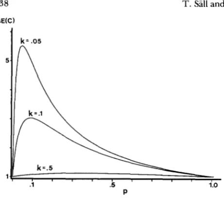
FIGURE 1.-Effect of meiotic heterogeneity in a backcross. Shown here is the relationship between the proportion p of gametes with a high recombination frequency and the expected estimated coefficient of coincidence, AsE(C).

segments. However, it can be shown that the value of AsE(C) in such a case falls between the values ofAsE(C) that are obtained if the maximum and the minimum of the two

k

values are inserted in Equation 10. Thus, no extra insight is gained by introducing this extra complexity. We will therefore not investigate these cases any further.

However, in case two, the heterogeneity leads to an estimated negative interference which could well be detected-with surprise-in a practical crossing experiment. T h e phenomenon also occurs if the variability in recombination frequencies differs between the two chromosomal segments. As in case three, different

k

values cause an effect that is intermediate to the effect given by the maximum and the minimum of the two

k

values. We have therefore made a detailed investigation of the properties of Equation 9 for different parameter combinations and, in particular, de- termined the maximum size it may take when there is no interference at the cytological level. We have also studied the effect of recombination variation when, within each gamete population, there is a “standard” amount of positive interference (as given by KOSAMBI

1944).

Negative interference due to variation in recom- bination frequencies: Equation 9 has several interesting properties. First of all it can be seen immediately that A s E ( C ) is independent of the recombination frequencies TAB and rBc. It can also be seen that A s E ( C )

= 1 for the trivial cases

p

= 1 or

p

= 0 and for the case

k

= 1 . However, for all other parameter configurations A s E ( C )

>

1 . Thus, heterogeneity in recombination fractions will cause an expected coincidence above one.

T h e dependence of AsE(C) on

p

loci so that L rBcI). It can then be shown that the maximum value becomes

AsE(C),,, = l/p = 1/2E(rAB). 1 ) ( 1

Thus, a large bias can be produced only when the investigated loci are closely linked most of the time but a small fraction of gametes is produced with much larger recombination values. T h e differing gametes must, however, be so few that the estimates of the recombination fractions in the total material remain small.

A comment on the variance of C should also be made for this case. Equation 4 shows that the variance of C is a third degree polynomial of c, which starts at zero, then either increases to a peak, drops slightly and then increases again for large values of c or increases all the time depending on the values of TAB and rBc. T h e positions of the peak and the valley, if any, also depend on the values of TAB and rBc. As a rule it can be said that the variance increases for small values of TAB and rBc. Thus, parameter configurations that create large values of AsE(C) and small values of and E(rBc) will also be associated with a large variance.

One way to study the effect on the variance is to consider the ratio between the variance of C in the case of heterogeneity and the variance of C with no heterogeneity, given the same average recombination frequencies. It can be shown that the ratio is always smaller than A s E ( C ) but approaches this value when the recombination values decrease.

Model with Kosambi interference: In the investigation above only the case without interference in any of the gamete populations has been considered. If interference is allowed, the complexity of the problem increases considerably. In the following we have investigated case two when the interference in the two gamete populations follows a specific type of interference, the KOSAMBI interference which is of the general form

(5)

Apparent Negative Interference 939

Q

1 .5

P

1.Q

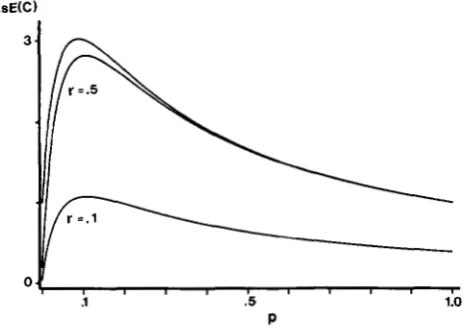
FIGURE 2.-Effect of KOSAMBI interference on the expected estimated coefficient of coincidence AsE(C). The effect is compared

to the case with no interference (the uppermost curve) for two values of r (where r = rABI = rBcI) over the range of p . The comparison is made for k = 0.1.

This interference has been chosen because it is one of the most simple and most widely used mapping func- tions considering interference. It has also, in a number of cases, shown a good fit to empirical data; see BAILEY

(1 96 1). For simplicity we have studied the case where

?-AB1 = rBcl = r. Thus, for cl, r has been inserted for

TAB and rBc in (1 2), and for cp kr has been inserted. In

Figure

2

the effect of the KOSAMBI interference is shown for

k

= 0.1 and two different values of r. For comparison the curve for

k

= 0.1 without interference is included. It can be seen that the effect on the estimated coincidence is of the same general form as when there is interference in the gamete populations, with only a slight shift in the position of the maximum. It is also evident that the value of A s E ( C ) is strongly affected by the value of r. For r = 0.5 the reduction in A s E ( C ) is very small for most values of

p ,

but for r = 0.1 the level of coincidence is strongly reduced.

Model with several gamete populations: So far a model with only two gamete populations has been considered. Let us now assume that the heterozygous parents produce n gamete populations 1,

. .

.,

n in the proportions

e,,

. .

.

,

p,,

with the recombination frequencies k i r A B and kirBC, where k l = 1, and ki I 1. Then the frequency in the total gamete pool of

-

k r A B ) , and

pikz 2 r A B r B C .

We assume here that there is no interference between recombination events in the two segments in any of the gamete populations. In analogy with ( 5 )

and (6) the estimators of the recombination frequencies have the following expectations

E(RAB) = TAB piki

E(&) = rBC

C

p i k ,

while the asymptotic expectation of becomes

the estimator C

This expression can be rewritten as

where V ( k ) stands for the variance of

k.

This is con- sistent with the earlier results: when V ( k ) = 0 the gamete pool is homogeneous so that A s E ( C ) = 1. In all other cases we expect to score A s E ( C )

>

1.

It is important to note that the largest variance of

k

for any recombination frequencies is achieved when there are only two gamete pOpUlatiOnS with r A B l = 0.5

and k p = TABZ = rBcz = 0. Thus, the upper limit that is set by (1 1) also applies to (13), so that the most dramatic effect of recombination variation occurs when there are two gamete populations having widely different recombination frequencies.

Model with selfing: So far the calculations have been applicable to the situation where haplotypes are scored, as in a backcross program. In self-fertilizing organisms linkage is usually studied by looking at the progeny of selfed heterozygous F1 individuals. For the present purpose there are two important differences between backcrosses and intercrosses such as the selfing of F1 individuals. In a backcross, as pointed out above, the gametes produced by the F1 heterozygotes can be scored immediately and used in the estimation of linkage. In an intercross, however, both chromosomes in an FZ individual come from a heterozygous FI individual and are thus informative. Secondly, the genotype of the gametes uniting in the F2 individual will normally not be known if there is dominance at one or more of the loci (unless the analysis is taken one generation further). This implies that the simple and intuitive estimators (1) and (2) cannot be used when the recombination frequencies are to be studied. Instead maximum likelihood estimates of the recombination frequencies must be derived from the proportion of different phenotypes in the FZ generation. T h e same method must also be used to estimate the coincidence. There are, unfortunately, no analytical solutions to these likelihood equations (RAO 1947), so

(6)

ASEC)

1

k = . 5 , p = . 3

1

.1 .S

5 6 1

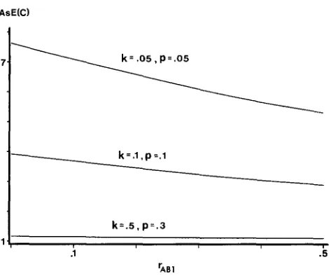
FIGURE 3.-Relationship between the recombination frequency,

T A B , , and the expected coefficient of coincidence, AsE(C), in the

case of selfing. In all cases the recombination frequencies are the same in segments A-B and B-C ( h = 1).

der identical recombination frequencies to see what happens when the gametes belong to different gamete populations instead. T h e type of cross we have considered is the case of selfing where the male and the female gametes have the same recombination frequencies in all fertilizations, but where there are recombination frequency differences between fertilization events. An example where this may occur is in a self- fertilizing plant where there are differences in recombination frequencies between different flowers depending on their positions in the influorescence, a situation that may occur in, e.g., barley.

T o investigate the effect of recombination variation on the coincidence estimate under selfing we have used the same model as in section “Negative interference due to variation in recombination frequencies” above. T h e likelihood equations for the estimate of coincidence and recombination fractions have been solved numerically for different cases, but here, we shall concentrate on the results obtained for the estimator of the coincidence. Only the situation with three loci and dominant alleles in coupling will be considered. As before, we assume that there is no interference in any of the gamete pools, so that any deviation from A s E ( C ) = 1 derives from the bias d u e to meiotic variation among the parents.

T o simplify the description of the effect of different

T A B 1 and rBcI values the factor h = rBCI/rABI is intro-

duced. We still assume that r A B l takes the larger value,

so that h 5 1.

The values given to AsE(C) by the standard maximum likelihood function are shown in Figures 3 and 4 for different values of ?“ABI, k , h and

p .

From the

figures it can be seen that, as before, a variation in recombination frequencies among fertilizations intro- duces a bias to the estimator of coincidence making its estimates greater than one even when no coinci-

FIGURE 4.-Comparison between the backcross and the selfing cases. In both situations a fraction 0.10 of the gametes has higher recombination values. The recombination frequencies are the same in both segments A-B and B-C ( h = 1). Two curves are shown for the selfing case, representing different levels of recombination. The backcross curve is labeled B.C.

dence exists in any of the gamete pools. It is also seen that a difference exists between the backcross and selfing cases. In particular, the value of A s E ( C ) under selfing turns out to be dependent on the recombination values (rABI and h ) as well as on

k

and

p .

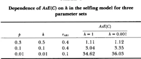
T h e dependence on h is illustrated in Table 1 for three combinations of parameters. T h e dependence is such that A s E ( C ) increases with decreasing h, but the effect must be considered to be small. T h e dependence of

AsE(C) on is illustrated in Figure 3, which shows

that A s E ( C ) increases with a decrease in T A B I . The

effect of a change in r A B l is clearly greater than a

change in h, especially for small k and

p

values around the maximum point for the curve. Still one should note that the effect is limited, as seen from Figure 3, i . e . , the function does not run away towards infinity for small TAB1 values.

Despite the difference between the backcross and the selfing situations, the two cases are basically similar in that

k

must be considered as the major determinant

of AsE(C). Figure 4 also shows that the general shape

of AsE(C) over

p

is the same for the selfing and the

backcross curves. For a given

k

they both stay within the same order of magnitude.

An interesting observation from the selfing case is that the expectation of the recombination value derived from the estimator RAB is not the same as the expectation for the backcross case [ i e . , rABI(p

+

q k ) ;

see (4)]. Thus, with variable recombination frequencies the standard maximum likelihood equation gives a biased estimate of the mean recombination frequency. Under selfing the E(&) value is always smaller than the corresponding value in the backcross. For our purpose, the most important question is

still: for a certain parameter configuration giving a particular value for E ( R A B ) and E(&), what is the

(7)

Apparent Negative Interference 94 1

TABLE 1

Dependence of AsE(C) on h in the selfing model for three parameter sets

AsE(C)

P k rA B1 h = 1 h = 0.001

0.3 0.5 0.4 1 . 1 1 1.12

0.1 0.1 0.4 3.04 3.35

0.01 0.01 0.1 34.62 36.03

answer this question a systematic study of different examples has been performed. T h e largest bias seems, as before, to occur for

k

= 0 and r A B l = 0.5. As E(C),,, is then numerically identical to the corresponding value in the backcross case, although the

p

values giving the maximum are not identical. This is illustrated in Table 2. If

k

>

0 or TAB1

<

0.5 then the maximum in the two cases are not exactly the same which also is illustrated in Table 2. It can be seen that either the selfing case or the backcross case gives the highest value of AsE(C),,,, depending on the case

considered.

DISCUSSION

A coefficient of coincidence greater than one is expected in a linkage experiment if the offspring arise from heterogenous meiotic events when there is a positive correlation between recombination frequencies along the chromosome. This holds for backcross experiments as well as for experiments based on selfing. In the case of selfing, only the situation with complete dominance at all three loci has been considered, since this is the most extreme case in comparison with a backcross. If there is codominance at one, two, or three loci in the selfing case, the information increases as we approach the situation where the genotype of each chromosome can be deduced. T h e re- sponse of AsE(C) on recombinational heterogeneity will then be more similar to the backcross situation.

A complete similarity is reached when each allele in the offspring can be traced back to its maternal or paternal origin. Such a case occurs, for example, in the study of seed markers in self-fertilizing plants where the dose effect in the endosperm allows for a complete scoring (see e.g. DOLL and BROWN 1979).

We have also shown that the effect of gametic heterogeneity on the estimated coincidence will be limited under most reasonable parameter configurations. In Figure 1 it is seen, for example, that a reduction of 50% of the recombination fractions in a part of the gamete pool has only a small effect on the coincidence. It is only when the reduction approaches 90% or more

(k

<

0.1) that a substantial effect is produced. It is then also required that the gamete population characterized by the larger recombination fraction is so small that it has only a small effect on the mean recombination fraction.

TABLE 2

Comparison of the selfing and the backcross cases with respect to the dependence of AsE(C),., on different combinations of

rml, k and p, given that E(rM) = 0.1

Type of ex-

periment k rA B 1 AsE(C),,,

Selfing 0 0.5 5.0

Backcross 0 0.5 5.0

Selfing 0 0.4 4.2

Backcross 0 0.4 4.0

Selfing 0.1 0.5 2.9

Backcross 0.1 0.5 3.0

For all examples shown, h = 1 . The values of AsE(C),,, in the selfing case are approximate. In neither of the three comparisons the maxima are obtained at the same p value.

Thus, only in special circumstances will a significant negative interference be found in a linkage experiment. This is true in particular if one considers that there may be positive interference in each of the sep- arate gamete populations. In the case of KOSAMBI

interference the effect is especially pronounced if and rBcz are small. If, on the other hand, the recombination frequencies are large, the reduction of

A s E ( C ) becomes quite small and the conclusions that

have been drawn above also apply to the case with

KOSAMBI interference.

Given these considerations one may ask whether the observed cases of (weak) negative interference in eukaryotes can be explained by the effect of meiotic heterogeneity. Years after an experiment was performed it is, of course, normally impossible to know whether any recombinational variation occurred in the material. A theoretical analysis can, however, be made to see whether a variation in the material could produce the observed results and find the amount of variation that must be postulated for the coincidence estimate to have the right expectation. It should be remembered that the estimator of the coincidence has a variance and that this variance increases with the expectation of the estimator; we will, however, restrict our analysis only to considerations of the expected value.

We have made such a reanalysis of the results reported by GREEN (1975) and SBGAARD (1977). Com- binations of

p ,

k

and r A B J have been found that give

the identical values for the recombination frequencies and the coincidence value obtained in their experiments. In Figure 5A the result of our reanalysis of the backcross experiment made by GREEN (1975) in Dro-

sophila melanogaster is described. T h e estimated re-

(8)

k

0,

.1 1 . 2 5

P

FIGURE 5.-Fitting the model to empirical data. Shown are possible combinations of parameters that will lead to the observed values for the coefficient of coincidence and the largest recombination frequency. The dotted line shows the values of the recombination frequency in the high recombination gamete population,

rAB,, and the solid line shows the needed variability in recombination frequencies, given by k . In (A) the data from GREEN (1975) has been fitted, where the Coefficient of coincidence was 1.56 and the largest recombination frequency was 0.039. In (B) the data from S ~ A A R D (1977) has been fitted, with a coefficient of coincidence of 3.4 and a largest recombination frequency of 0.095.

derived from meioses with four times the normal recombination rate. T h e negative interference observed in this case may thus be due to a variation in recombination rates; we are not, however, able to judge how likely it is that such a variation existed in

the material that was used for the experiment. In the case of the barley experiment reported by SBGAARD (1 977) the estimated recombination frequencies were 0.095 and 0.030, while the estimated coefficient of coincidence was 3.4. Our reanalysis of her data is given in Figure 5B. In this case more

drastic variation is needed to produce the observed values. For example, it is necessary to assume here that some meioses had recombination frequencies that were more than 10 times larger than the normal values (ie.,

k

must be smaller than 0.10). In experiments currently under way we study whether such extensive variation in recombination frequencies is normal in barley plants, for example between flowers in different positions in the spike or between primary and secondary spikes.

We wish to thank 0. HAGRING for his help in making the computer programs, G. LINDAHL, B. GILES and N. BARTON for comments and advice on the manuscript and P. E. ISBERG for helping us produce the graphs. We also like to thank J. LANKE for advice on expectations of ratios. Finally we would like to thank L. BROOKS and two anonymous referees for advice. This work has been supported by the Swedish Council for Forestry and Agricul- tural Research and the Swedish Natural Science Research Council.

L I T E R A T U R E CITED

AMATI, P., and M. MESELSON, 1965 Localized negative interference in bacteriophage X. Genetics 51: 369-379.

BAILEY, N . T . J., 1961 Introduction to the Mathematical Theory of Linkage. Clarendon Press, Oxford.

CHASE, M., and A. H. DOERMANN, 1958 High negative interference over short segments of the genetic structure of bacteriophage T4. Genetics 43: 332-353.

DOLL, H., and A. H. D. BROWN, 1979 Hordein variation in wild

Hordeum spontaneum and cultivated H . vulgare barley. Can. J. Genet. Cytol. 21: 391-404.

GREEN, M. M., 1975 Conversion as a possible mechanism of high coincidence values in the centromere region in Drosophila. Mol. Gen. Genet. 1 3 9 57-66.

KOSAMBI, D. D., 1944 The estimation of map distance from recombination values. Ann. Eugen. 12: 172-175.

LARSSON, H. E. B., 1985 Linkage studies with genetic markers and some laxatum barley mutants. Hereditas 103: 269-279. MORGAN, T. H., A. H. STURTEVANTand

c.

B. BRIDGES, 1925 The

genetics of Drosophila. Bibliogr. Genet. 2: 1-262.

PRITCHARD, R. H., 1955 The linear arrangements of a series of alleles in Aspergillus nidulans. Heredity 9: 343-37 1 .

RAO, C. R., 1947 Methods of scoring linkage data given the simultaneous segregation of three factors. Heredity 1: 37-59. S ~ C A A R D , B., 1977 The localization of eceriferum loci in barley.

V. Three point tests of genes on chromosome 1 and 3 in barley. Carlsberg Res. Commun. 42: 67-75.

STAHL, F. W., 1969 The Mechanism of Inheritance. Prentice-Hall, Englewood Cliffs, N.J.

STEVENS, W. L., 1936 The analysis of interference. J. Genet. 32:

51-64.

STREISINGER, G . , and N. C. FRANKLIN, 1956 Mutation and recombination at the host range genetic region of phage T2. Cold Spring Harbor Symp. Quant. Biol. 21: 103-1 1 1 .

SUZUKI, D. T., A. J. F. GRIFFITH and R. C. LEWONTIN, 1981 An

Introduction to Genetic Analysis. W. H. Freeman, San Francisco. VISCONTI, N., and M. DELBRUCK, 1953 The mechanism of genetic

change in phage. Genetics 38: 5-33.

VON WETTSTEIN, D., S. W. RASMUSSEN and P. B. HOLM, 1984 The synaptonemal complex in genetic segregation. Annu. Rev. Ge- net. 18: 331-413.