Public Logistics Network Cost Analysis

(1)

ABSTRACT

CHIN-LING HO, Public Logistics Network Cost Analysis. (Under the direction of Dr.Michael G. Kay )

A public logistics network (PLN) was proposed as a means to allow multiple firms to cooperate in providing ground parcel transport. To support fast and flexible shipping, a PLN would require sorting in terminals. In this research, we address to find an upper bound on the terminal cost for a PLN system such that its total transport costs would be the same as that of the a private logistics network like UPS. The labor costs in current terminals are high because of lots of human handling [10]. In order to reduce high labor costs and provide efficient sorting capacity, we want to use automatic equipment in the PLN terminals.

Since the biggest parcel delivery company, UPS, is a hub-and-spoke (HUB) transportation system, the total logistics network cost in a PLN should be higher than UPS’s. The total logistics network cost includes line-haul transportation cost, pick-up/delivery (P/D) routing cost, and terminal cost. By analyzing each cost in the logistics network, we define an upper bound terminal cost for a PLN based on a similar level of service with HUB. A hypothetical network of 36 terminals in the southeastern U.S. is used as an example PLN in the analysis.

(2)

Public Logistics Network Cost Analysis

by

CHIN-LING HO

A thesis submitted to the Graduate Faculty of North Carolina State University

in partial fulfillment of the requirements for the Degree of

Master of Science

INDUSTRIAL ENGINEERING

Raleigh

2005

APPROVED BY

Robert E. Young

Jeff Thompson

Michael G. Kay

(3)

BIOGRAPHY

(4)

ACKNOWLEDGMENTS

I sincerely would like to thank Dr. Michael Kay, my advisor and chairperson of my thesis committee, for his patience in teaching, explanation, and stimulating suggestions during the work. He has devoted so much time and effort to teaching me both in this research and in writing the thesis.

I am grateful to my thesis committee members Dr. Young, and Dr. Thompson for spending time reading the thesis and giving me invaluable advice.

I have to thank my parents, my brother and my sister for your love that encourage me to do my second master degree.

(5)

1. Introduction

With the increase of e-shopping and e-commerce business, companies or individual sellers need to provide short-transport-time and low-cost shipping services by outsourcing their logistics system [25]. The increase of competition in the transportation market requires the cooperation between third-party logistics [6]. They often use distribution centers, warehouses, or terminals to consolidate products or shipments. A distribution center is the place for receiving parts from suppliers, storing products, and distributing products to buyers. A warehouse is the place for a company to manage its inventory and to deliver products to its buyers. A terminal is the transshipment point for loading and unloading products.

A Public logistics network (PLN) is designed for the ground delivery to transport parcels [15]. In a PLN, public warehouses are used as terminals to operate ground parcel shipments, including sorting, loading/unloading, and consolidating packages. This research defines the logistics network cost for these public warehouses, including line-haul transportation cost, pick-up/delivery (P/D) routing cost, and terminal cost. However, it is difficult to evaluate the terminal cost due to unknown demand, the location of terminals, and technology expenses. We plan to use UPS experience to approximate the logistic network cost and then determine the terminal cost for a PLN.

(10)

handling, like a HUB system, it would have higher terminals cost than the HUB system. In order to reduce a PLN system cost, sorting and scanning packages should be operated automatically without any human handling.

It is a challenge to estimate cost for the automatic terminal when there is no such terminals in the current parcel industry. Therefore, this research tries to find an upper bound cost to invest PLN terminals without paying more costs than UPS. We address finding the upper bound of sorting asset cost for a PLN by assuming as the same total logistics network costs as a HUB system. The upper bound cost will be used to evaluate the investment plan for a PLN. Before delving further into the PLN cost analysis, the current parcel industry and the related research will be reviewed.

1.1 Parcel Industry

Parcel service, one of the services in the freight transportation, is a professional delivery service that primarily conveys parcels in accordance with a fixed, defined transportation program, by using logistics networks with fixed running times for their specific goods [31]. The size of a parcel is small enough to be handled by one person without aid, but normally larger than a single letter [3]. There are multiple transportation modes, which include air-cargo, railroad, water, pipeline, and truck in parcel service to cover wide regions and provide diverse services.

Mode Comparison

To choose a transportation mode for a particular shipment, the distributor must consider shipment sizes, feasible arrival dates for customers, and transportation costs [8]. The criteria of the mode selection include cost, service, and the type of packages. The advantage and disadvantage of transportation modes are presented in Table1.1.

(11)

mode and it is very expensive. It charges a high price for very high quality services, like emergency and national shipments. The operation of air cargo relies on trucks to support transportation from the airports to other ground transshipment points.

Water/Ocean shipping is widely used for international long-haul commodities. There are two kinds of commodities in ocean shipping, dry and wet. Wet commodity is mostly oil products and dry commodity can be anything else. Comparing with railroad freight car and trucks, these ships are enormous but slow. In contrast to air transportation, water mode tends to be relatively inexpensive per unit weight and per unit distance.

Railroads are used for low value freight, such as coal transport, that does not require high level-of-service shipments [30]. Due to economic considerations, companies need to gather enough traffic so that trains can be operated as a long train. Cost per freight car on a long train is much lower than on a short train, but the train operating costs increase with train length.

(12)

which freight modes are chosen. Some shipping services named with Air, like UPS Next Day Air Saver and UPS Next Air Early, might also use rail or truck. Trucking is the most important modes in shipments. It is called ground delivery.

Table 1.1 Comparison of different transportation modes

Mode Advantages Disadvantages

Air

Faster service

International/national

Expensive price

Truck support needed

Schedule is not flexible

Rail Low price

Slower service than trucks

Water

Low price

International/national

Slowest service

Truck/Ground

Low price

Schedule is flexible

More expensive than rail

Ground Delivery

(13)

storage and consolidate shipping. Due to the different operations in TL and LTL, the prices charged from shippers are different as well. TL shipping is priced by truckers who ship goods such that they can get enough profit. LTL pricing is more complex because of its higher capital

investment [30]. Therefore, LTL cost analysis is worth studying. Nowadays, more and more LTL haulers are making headway among shippers that move

large volumes of small packages to business consignees [29]. Some LTL haulers are associated with parcel and express specialists, such as delivery within specific time window, time-definite or day-definite. A trend of integrating public warehouses and LTL haulers is observed in the expansion of the small package delivery market. The PLN was proposed as a means of extending many features associated with public warehouses and LTL companies to enhance economical scales of shipping. This research will try to help LTL companies to analyze their investment costs on terminals.

Terminals in Parcel industry

(14)

loading/unloading packages and traffic congestion, might cause the increase of indirect cost for terminal operation.

FIGURE 1.1 PARCEL FLOW IN POSTAL CENTER [14]

1.2 Logistics network related research

Logistics researches have been widely studied in business aspect and production aspect. This research classifies these related research topics into shippers, handlers, and carriers.

1. Shipper: delivery time and shipping cost

Nowadays, many manufacturers and retailers seek to outsource their logistics services to short lead-time or reduce cost. How to select motor carrier and service capability has been concerned in the carrier selection process, especially for the cost minimization [2]. The shipping cost with freight rate or lead time is examined in Economic Order Quality (EOQ) model for the inventory policy of supply chain companies [33].

2. Handlers: sorting technique and warehousing design

The use of terminals between plants/suppliers and customers allows the concentration of shipments to increase the flow on these links and to generate economies of scale by improving

Discharge

Counter

Storage Circular Flow Sorting

Storage Shipping

Delivery

Truck arrivals

Truck Departures

(15)

the vehicle load [21]. Two issues about sorting and warehouse layout design have been studied to improve the efficiency of terminals. First, sorting process is critical to reduce transportation time, save operating cost, and conserve resource [24]. Second, planning terminal layout is discussed to improve terminal efficiency and transportation time. Mathematical algorithms and heuristics were widely used for reducing operation cost of terminals and customer service cycle time [8] [18].

3. Carriers: vehicle routing and location of warehouse

Operations research has been used in finding optimal routing to deal with time-window and waiting cost [19]. In order to minimize overall cost, locations of warehouse and network modeling have also been studied [11]. Some researchers use simulation in the shipping system to describe network system [4].

Moreover, logistics cost have been investigated for various aspects. For example, the expected annual logistics cost is the summation of transportation cost, holding cost, ordering cost, and shortage costs in supply chain management [9]. For container, the operating costs for transportation are divided into three components: the routing costs, the resource assignment costs (driver/vehicle), and the container repositioning costs [17]. A cost function of LTL motor carrier, presented in the paper of Bruce [22], is the summation of labor cost, fuel cost, purchased transport cost as well as capital cost. Those studies help us to know which costs are important for different users, but they do not provide terminal cost for the parcel delivery. This research can expand logistics network studies to terminal area.

1.3 Overview

(16)

(17)

2. Public Logistics Network

In this chapter, the difference of routing paths and sorting points between HUB and PLN is discussed. Also, a UPS financial report is used for managers to see asset values and average transport costs in parcel delivery companies.

2.1 Hub-and-Spoke (HUB) vs. Public Logistics Network (PLN)

The HUB transportation system is widely used in telecommunication, air transportation and parcel delivery networks. The line haulage of a HUB includes package shipping within hubs and from terminal to the origin of hub as well as from the hub to the destination of terminal. Each non-hub terminal is allocated to the closest and exactly one hub. Packages are only consolidated and sorted in the hub.

A HUB system is treated as a very cost-efficient system for global logistics by using multiple modes of transportation systems [17]. Most parcel companies use a HUB system to speed up both ground and air parcel service, but this kind of pure HUB networks is not the only network structure for trucking shipments. A hybrid HUB system was proposed to save more cost of line-haul than pure HUB system [6]. It shows that there exist other logistics network systems which may use lower cost by changing routing paths.

(18)

Recent PLN research found that transport time of line haulage, including loading/unloading time, wait time, and transportation time is shorter in a PLN than in a HUB when the loading/unloading time is short [15]. Although both a HUB and a PLN are using Dijkstra’s algorithm in line-haul routing, the routing paths would be changed with the sorting places that routing assigned. Using a network linking 18 terminals as an example, we illustrate the shortest routes in Figure 2.1(a) for the HUB system and in Figure 2.1 (b) for the PLN system.

FIGURE 2.1 (A) HUB LINE-HAUL ROUTE; (B) PLN LINE-HAUL ROUTE

Line haulage of a HUB system or a PLN system can be denoted as shipping packages from terminal i to terminal k. For the HUB system, three terminals function as hubs to sort packages and the other terminals are used to collect local packages only. For PLN the system, all these 18 terminals operate as smaller hubs to sort passing packages. By using the Dijkstar’s algorithm, both

Terminal (b)

i

k

j w

Terminal Hub (a )

i

k

1

2

3

(19)

HUB and PLN would pick the same routes for traveling a pair of terminals. Due to the sorting at different places, the trucks in the PLN could travel shorter but stop more terminals than in the HUB. The routes of the HUB and the PLN are described respectively:

HUB system:

Routing:

Sorting: Packages are sorted in hub1 and hub3 PLN system:

Routing:

Sorting:Package are sorted in terminal i, terminal j, terminal w, and terminal k

2.2 United Parcel Service (UPS)

UPS is the most successful parcel delivery among five large U.S. parcel industries: Airborne, DHL, FedEx, UPS and United State Postal [25]. To investigate current biggest parcel delivery company (UPS) will help us to define the logistics network cost in parcel industry. Their annual revenue the truck-based transportation represent that UPS is the largest domestic parcel carrier [31]. UPS uses a HUB system to deliver more than 14 million parcels per business day across the U.S. Its financial report would offer related logistics network costs for the HUB. Next we will discuss their transportation system, domestic service and service rate to provide a clear overview for ground delivery.

2.2.1 UPS transportation system

UPS is a hub-and-spoke system and has seven hubs in the U.S.: Louisville, Ky. (main U.S. Air Hub), Philadelphia, Pa., Dallas, Texas, Ontario, Calif., Rockford, Ill., Columbia, S.C., Hartford,

Terminal i Terminal hub 1 w Terminal k Terminal k

hub 3

(20)

Conn. All UPS goods-air and ground, domestic and international, commercial and residential services share the same network and infrastructure. Sharing infrastructure is very efficient and low-cost to use assets. A single network provides the flexibility to transport goods by using the most reliable and cost-effective transportation mode or combination of modes. Since UPS is one of the largest railroad customers in the United States [25], shipments are handled at a lower cost per package with fewer miles traveled between stops.

Four main UPS operations are pickup, sorting, line-haul feeder service, and delivery. The package pickup process is available for regular customers, drop boxes, and call-ins. Packages are aggregated in local operating centers and sorted according to ZIP codes, waiting for shipping to terminals. The inbound packages are delivered to customers during daytime, and outbound packages are collected in the evening after truck shipping is finished

2.2.2 UPS Domestic Service

UPS operates 185,000 trucks in its ground network and uses a fleet of larger vehicles to transport parcels between sorting hubs [25]. UPS provides every driver a specifically designed vehicle and all fuel, oil and maintenance. In the peak time, UPS leases additional trucks to support its transportation needs. All trucks, drivers, carriers, labors, and terminals are part of expenses in maintaining logistics network system.

(21)

package delivers more than 12 million packages with 88,000 vehicles [28]. The reason of this high percentage is the increase of shipping volume and price rate (Appendix D). U.S. domestic package financial data are organized in Table 2.1: revenue (R), operating profit (P), daily package and operating days.

Table 2.1 U.S. domestic package segment information, UPS 2004 Financial Report

U.S. domestic package

Revenue $26,610,000,000

Operating profit $3,345,000,000

Long-lived asset $15,971,000,000

Daily demand (units) 12,780,000

Operating day 254

Operating expense(R - P) $23,265,000,000

Revenue per piece $8.20

Operating cost per package $7.17

(22)

Table 2.2 UPS Operating Expenses, 2004, 2003

2004 (in millions)

2003 (in millions) Compensation and benefit $20,916 $19,327

Repairs and maintenance $1,005 $955

Depreciation and amortization $1,543 $1,549

Purchased transportation $2,059 $1,828

Fuel $1,416 $1,050

Other occupancy $751 $730

Restructuring charge and related expense – $9

Other expense $3,902 $3,591

Total $31,593 $29,040

On the other hand, assets in the financial report are composed of current assets, fixed assets, prepaid pension goodwill and etc. Long-lived asset information was provided in the “Geographic information” and divided into two parts: domestic and international. The long-live asset of “U.S. domestic package” is $15,971 million, which accounts for 80.7% of consolidated long-live assets in UPS. Detail of “property plant and equipment” from consolidated financial statements are provided in Table 2.3.

(23)

Table 2.3 UPS Property, Plant, and Equipment, 2004, 2003

2004 (in millions)

2003 (in millions)

Vehicle $3,784 $3,486

Aircraft $11,590 $11,897

Land $760 $721

Building $2,164 $2,084

Leasehold Improvement $2,347 $2,219

Plant Equipment $4,641 $4,410

Technology Equipment $1,596 $1,495

Equipment under operating lease $57 $53

Construction-in-progress $539 $450

Accumulated depreciation and amortization ($13,505) ($12,516)

Total $13,973 $13,298

2.2.3 UPS parcel cost

(24)

Table 2.4 UPS domestic package with services

U.S. domestic package Daily Package Package % Revenue per package

Next Day Air 1194000 9.34% $19.92

Deferred 910000 7.12% $13.68

Ground 10676000 83.54% $6.42

Total/ Expected Value 12,780,000 $8.20

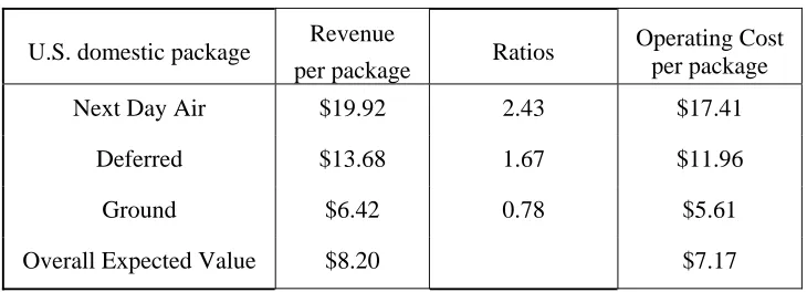
In Table 2.4, the overall revenue of “Next Day Air” services is $19.92. The delivery by Deferred usually needs 2–3 days and its revenue per package is $13.68. Generally, the delivery by Ground service needs 3–5 days and its average revenue per piece is $6.42. The average price of these services can be called as the revenue per piece, and the cost of these services should be lower than the revenue. Since the costs were not provided by UPS financial report, an approximate method is needed to obtain the specific operating expense for different services.

Next we use a simple method to approximate cost per package. First, we assume that the ratios of cost per piece are equal to that of revenue per piece for the three US domestic services. The ratio of a service revenue is computed as the revenue per piece for a service divided by domestic revenue per piece $8.20, and then we get 2.43 for “Next Day Air,” 1.67 for “Deferred,” and 0.78 for “Ground.” Multiplying these ratios with the U.S. domestic cost per packages, $7.17, the average cost per package for each of these three services are calculated and shown in Table 2.5.

Table 2.5 UPS “U.S. domestic” cost by services

U.S. domestic package Revenue

per package Ratios

Operating Cost per package

Next Day Air $19.92 2.43 $17.41

Deferred $13.68 1.67 $11.96

Ground $6.42 0.78 $5.61

(25)

Since the price of UPS is always varied with weight of package and traveling distance, the cost of UPS must be also varied with the weight of package and traveling distance. The price charts may be able to provide a basis of package costs for different weights and distances.

UPS processes the price rates of shipments by determining the size and weight of package and then determining the rate of service and the price zone. We organized the ground residential chart as an example in Table 2.6. Weights were ranked from 5 to 70 pounds by the increment of 5, and zones were provided from zone 2 to zone 8. We observed that the price per package is higher if the weight of package is heavier or the traveling distance is longer. Furthermore, we represent the pricing relationship between zone and weight in Figure 2.2. In Figure 2.2, each line represents prices in one zone.

The price is positively related to the package weight and the zone. Packages shipped in smaller zones are always charged less than in larger zones for traveling less distance. We observed that the price changes significantly at the weight of about 70 lbs. When the weight of package is less than 70 lbs, the slopes of smaller zone are less than the slopes of larger zones. These trends show that prices are affected by traveling distance more than by weight when weight of package is less than 70 lb. In contrast, when the weight of package is over 70 lbs, prices increase with a same slope. That shows prices are affected by the weight of human’s moving limitation.

(26)

Table 2.6 2005 UPS Ground Residential price and zone, in dollar

lb \ zone 2 3 4 5 6 7 8

5 5.56 5.79 6.47 6.67 7.02 7.25 7.85

10 6.35 6.45 7.08 7.47 8.05 8.87 9.88

15 7.08 7.39 7.64 8.24 9.82 11.53 13.07

20 7.61 8.38 8.68 9.8 11.96 14.07 16.28

25 8.36 9.42 9.94 11.39 14.14 16.62 19.52

30 9.17 10.37 11.24 12.96 16.33 19.12 22.68

35 9.84 11.38 12.54 14.57 18.47 21.79 25.9

40 10.53 12.41 13.81 16.19 20.48 24.45 28.99

45 11.15 13.39 15.02 17.81 22.33 27.08 32.02

50 11.62 14.23 16.05 19.26 23.84 29.36 34.57

55 12.1 14.83 16.96 20.47 25.19 30.9 36.35

60 12.58 15.42 17.73 21.45 26.44 31.73 37.55

65 13.06 15.95 18.35 22.13 27.34 32.62 38.75

70 13.5 16.48 18.93 22.81 28.15 33.5 39.94

0 10 20 30 40 50 60

0 20 40 60 80 100 120

weight of pacakge, Lb

pr ic e , $ zone2 zone3 zone4 zone5 zone6 zone7 zone8

(27)

3. Cost Analysis

This section proposes an analytical procedure to calculate costs in parcel industry. The procedure is to define the upper bound on sorting equipment cost that a PLN might spend. The assumption is that the total logistics networks cost of a PLN is as low as that of a HUB system. In the previous chapter, operating expense, asset cost, and package costs are discussed for a HUB system. In this chapter, the logistics network cost structure, cost formula for line-haul transportation and local pick-up/delivery (P/D) routing, economical transformation between operating cost and asset cost will be discussed. These discussions help managers equally to measure logistics network costs for both HUB and PLN system.

3.1 Defining Logistics Network Cost of Parcel Delivery

The logistics network in the parcel industry is a network in which terminals are linked to transport parcels. The logistics cost for a carrier is computed as a composition of the cost for drivers and vehicles to make pickups and deliveries (Pick-up/Delivery routing), the line haul cost for transporting freights between terminals (Line-haul transportation) and the handling cost for sorting and consolidating freight (Terminals) [10]. Other related researches considered logistics operations as line-haul operations, local P/D operations and terminal operations. In this research, we also consider these three operations in the evaluation of the logistic network cost.

(28)

decrease shipping cost, packages are aggregated into one large unit in the line-haulage and increase the economic scale in terminals. When packages arrive at the destination terminal, they wait until being delivered to individual customers. However, resources (vehicles, handlers and drivers) of the line haulage and the P/D routing are separated. Cost of the logistic network is the summation of line haulage cost and pick-up/delivery routing cost.

FIGURE 3.1 LINE HAULAGE AND PICK-UP/DELIVERY ROUTING

From the financial point of view, the logistics network cost for a parcel delivery company is associated with operating expense and asset costs. Before starting business, companies need to invest asset cost such as lands, buildings, equipment or machines to support their business operations. Operating expense in the company’s income statement is a catchall for every expense in that accounting year. Hence, total logistics network cost for a parcel deliver company should include the initial asset cost and daily operating cost. Based on parcel movements and financial needs, all the costs in the logistics network are listed and organized in Figure 3.2.

Terminal

_{Customer/drop box}

Line haulage (Stage 1)

(29)

FIGURE 3.2 COSTS OF LOGISTICS NETWORK SYSTEM FOR PARCEL DELIVERY

Based on the movement of parcel, the logistics network cost can be separated as line-haulage and P/D routing. From a financial point of view, the logistics network cost is divided into operations and assets. For example, the terminal equipment cost can be defined as a part of line haulage cost or a part of asset cost.

For the convenience of calculation, the logistics network cost structure is reorganized as shown in Figure 3.3. The movements of a parcel delivery are in the top of the structure. Also, terminal operating cost and terminal asset cost are condensed into a terminal cost. We calculate the logistics network cost as the summation of line-haul transportation cost (1), P/D routing cost (2) and terminal cost (3).

Line haulage Pick-up/Delivery Operating

Expenses

Assets

♦ Line-haul Transportation

♦ Terminal Operating cost ♦ P/D Routing

♦ Terminal Equipment

(30)

FIGURE 3.3 LOGISTICS NETWORK COST STRUCTURE

3.2 Analytical Procedure

After illustrating the structure of logistics network cost, we propose a procedure to explain the relationships among individual costs. The analytical procedure has three steps: input constraints, compute costs, and approximate a PLN upper bound sorting costs (Figure 3.4). Specifically, step 1 allows a company to input its constraints, step 2 computes all individual costs in logistics network cost, and step 3 uses the results from step 2 to provide the possible upper bound of sorting equipment costs for the PLN system and the transportation cost for each parcel. Since having different units between operating cost and asset cost, defining present value of logistics network cost can lead us find the upper bound asset cost for PLN. Since they are not consistence in units, a cost transformation with economic formula will be applied to solve the problem.

Logistics Network Cost

Line haulage Local Pick-up/Delivery Transportation Cost (1) Routing Cost (3)

Terminal Cost (2)

(31)

Line-haul Transportation Cost ($/ day) ($/year)

• HUB system • PLN system

Pick-up/Delivery routing cost ($/day) ($/year) • HUB system = PLN system

Step 2: Compute costs

Present Value

• Operating cost ($/year) • Asset cost ($)

PLN costs

• Upper bound sorting cost ($) • Parcel transport cost ($/piece)

Step 3: Estimate PLN Upper bound costs

Total Daily Demand Proximity factor (p-factor) Loading weight of truck Expected Package Weight

Step 1: Input constraints

Terminal Cost ($) • HUB system

(32)

The details of the analytical procedure are described as follows. Step 1: Input Constraints

Before a company starts evaluating its logistics network cost, constraints are required for the transportation demand and number of trips for truck schedules. From demand and the number of trips, we can generate the number of trucks, the number of carriers, the gallons of gasoline, and the number of sort needs in the line-haul transportation.

• Proximity factors: The proximity factor controls the extent to which a terminal is more likely to transport packages to nearby terminals as opposed to terminals located further away. The demand weight between each pair of terminals is estimated by using the population percentage of each terminal together with a proximity factor, wij. When the proximity factor is bigger,

there are more nearby shipments and shorter traveling distances [15]. • Total daily demand: The total number of packages delivered in a day.

• Expected Package Weight: An expected weight for all delivered packages in the network system.

• Loading weight of trucks: The maximum capability of a line-haul deliver truck. Step 2: Compute costs

The logistics network cost, including line-haul cost, P/D routing cost and terminals cost, for both a HUB and a PLN, is computed in the step 2. First, line-haul transportation cost is computed by following the different path for both a HUB and a PLN. Then, by letting the HUB and the PLN system use the same P/D routes, we simplify the calculation of the P/D routing cost. For computing terminal cost, we respectively consider terminal operating cost and terminal asset cost for HUB and PLN. The detail of cost calculations will be provided in the next cost sections.

(33)

To estimate the PLN upper bound cost, operating cost and asset cost are needed. However, the calculated costs are not consistent in units. The operating cost usually is represented as dollars per year ($/year), and asset costs are represented as dollars ($). In order to operate these costs, finding present value for the operating cost is needed. This research uses an economical formula to recalculated the value of operating cost according to the useful life of used assets.

The way to estimate the PLN terminal cost is based on the assumption that total logistics network cost in PLN is equal to the logistics network cost in HUB. We evaluate the difference between operating cost of the HUB and the PLN system. Summing the difference of operating cost and origin asset cost of HUB, the upper bound of PLN terminal cost can be found. Transportation cost, including line-haul transportation cost and P/D routing cost, will be used to calculate the average parcel transportation cost. The purpose of calculating average parcel transportation cost is to validate logistics network cost in a HUB by comparing it with UPS prices.

3.3 Transportation Cost

(34)

system. The details of how to calculate line-haul transportation cost and P/D routing cost are discussed in the next section.

3.3.1 Line-haul Transportation Cost

Line-haul transportation cost depends on line-haul truck operations such as truck rental/purchased fee, fuel cost, and driver cost. These costs are incurred according to the number of trucks, the number of carriers, and the gallon of gasoline, and vary with truck capacities and proximity factors. Some notations are defined:

TC: Average truck rental /purchased cost per day FP: Fuel price per gallon

CS: Daily carrier salary NT: Total number of trucks NG: Total gallon of gasoline NC: Total number of carriers

Line-haul Transpiration Cost Model,

CL

(35)

operating hours and shipping speed. The number of truck is rounded up to an integer. When a truck arrives at terminal f, all packages are unloaded, and another truck comes to ship the packages to terminal j. Therefore, the number of truck required in one trip is 2 trucks, i.e., 250 / (60 ×8) = 1 plus 350 / (60×8) = 1. The number of trucks is computed as the number of trips multiplied by the number of trucks required for a trip. In this example 4 trucks are required since 2 trips × 2 trucks/ trip = 4 trucks.

FIGURE 3.5: NUMBER OF TRUCK INTERPRETATION

Similarly, the number of carriers is calculated as the number of trips multiplied by the number of carriers in one trip. Assuming that a carrier drives 8 hours a day with the speed of 60 mph, then the number of carriers is 4 as well. The gallon of gasoline used is calculated as total travel distance divide by the average miles traveled per gallon.

3.3.2 Pick-up/Delivery (P/D) routing cost

Since the same demand and P/D routes are assumed, P/D routing cost would be the same in both a HUB and a PLN. Two actions in P/D routing are delivering packages to customers and picking up packages at the stops by local vans. We believe that the cost of vans for picking up packages could be omitted because no matter how far a van travels, the van should pick up all of

1000 units of 10 lb package Teri

Terj

250 miles

: 5000 lb : 8 hours : 60 mph Terf

(36)

the P/D routing cost in the whole logistics network. Just like line-haul truck, cost of vans is spent on the rental/purchased truck, gasoline, and one driver payment.

Some notations are defined:

VC: Van rental/purchased cost per day FC: Fuel cost per van per day

TD: Total daily demand in the logistics network D: Average-handling packages per van per day P/D routing cost model, CPD:

(

)

D TD CS FC VC

CPD= + + × (3.2)

The total P/D routing cost is the number of vans multiplied by the cost of one van. The number of vans is determined as the daily demand divided by the average delivering packages per van. From equation 3.2, the larger the handling packages can be, the less the P/D routing costs would be.

3.4 Terminal cost

In Figure 3.3, terminal operating cost and terminal asset cost are put into terminal cost. Terminal operating cost is used to represent the cost for the daily operation in terminal such as labor and handled cars. Terminal asset cost represents buildings, technology equipment, and plant equipment based on the present values of assets after deduction. As has been mentioned, the total logistics network cost of the HUB system, including transportation cost and terminal cost, is what is to be set for the PLN system. Terminal cost of the HUB should be computed first.

3.4.1 HUB system

(37)

percentage of line-haul transportation, we can approximate the terminal operating cost. The operations in hub (or terminal) mostly are proportional to the needs of transfer. When line-haul transportation is heavy, the operations in terminals are even heavier due to the need to cooperate with truck schedules. On the report of Wanser and Zapfel [16], he presented the parcel delivery service with complete geographic coverage for a HUB system:

• Line-haul transportation: 15–25% • Pickup and delivery costs 35–60%

• Depot (terminal) Operating cost: 25–45%

(38)

FIGURE 3.6 TERMINAL COST OF HUB SYSTEM 3.4.2 PLN system

For the PLN system, the terminal operating cost is zero because terminals are assumed to be fully automatic. Depending on the cooperation of plant equipment and technology equipment, the automatic sorting equipment should move and scan packages at the same time. However, since automatic terminals do not exist, we are not sure of what type of assets or equipment are needed. Depending on the same logistics network cost with a HUB system, which includes transportation cost and terminal cost, the discrepancy of transportation cost could be used to compensate for the HUB terminal cost. The process to calculate PLN terminal cost is shown in Figure 3.7.

Compute HUB Line-haul Transportation cost ($/year)

Define % of line-haul transportation cost for terminal

Operating cost ($/year) ($/year)

HUB Terminal cost ($)

Add HUB terminal Asset cost ($)

(39)

FIGURE 3.7 TERMINAL COSTS OF PLN SYSTEM

Once the line-haul transportation costs and P/D routing costs are computed, the difference of operating cost between the HUB and the PLN can be obtained. The information can provide the annual PLN saving in transportation. Transforming this difference of transportation cost in dollar based on the useful life of assets, adding it to the terminal cost in HUB, the PLN terminal cost can be generated. This terminal cost is an upper bound cost, below which the PLN manager can consider to import terminal assets.

3.5 PLN upper bound cost

After the PLN terminal asset cost is computed, the upper bound cost about terminal sorting cost is found. As we mentioned before, sorting is needed before a truck arrives in a PLN terminal. Terminal assets are designed to support the sorting. In order to fully use the capacity of a terminal, the size of the terminal should be evaluated. Generally, the size of a terminal can be divided into storage area and handling area as shown in Figure 3.8. Trucks unload packages in the

Add to HUB terminal asset Cost ($)

Compute operating cost difference ($/year)

Get PLN asset terminal cost ($)

PLN terminal asset cost = PLN terminal cost

(40)

the trucks, a sorting technology that robot arms pick up packages from the storage area, scanning them and put them on the handling area. The more trucks pass by the terminals, the sorting equipment are busier. Company should set more sorting equipment for the terminal where lots of transfers are needed. Finding a cost of sorting per truck stop is very helpful to determine the size of terminal for their demand and location.

FIGURE 3.8 TERMINAL LAYOUT

The more sorting needs of a terminal, the more PLN should invest on its sorting equipment. The cost of sorting per truck stop is terminal asset cost divided by the daily number of sorting needs in a day. To calculate the number of sorting needs in the logistics system, we count the number of truck stops in line-haul transportation by MATLAB.

TAC: PLN upper bound terminal asset cost in whole logistics network ($) NS: Daily number of sorting needs in the logistics network.

UBC: Upper bound sorting cost per truck stop ($)

NS

TAC

UBC

=

÷

(3.3) Divide the upper bound terminal asset cost by the daily number of sorting needs, the upper bound sorting cost per truck stop is calculated. This upper bound sorting cost is an average value for overall logistics network system. The more daily number of sorting needs are in the logistics

Storage Area

Handling Area

Arrive & Unloading

(41)

system, the lower the upper bound sorting cost per truck stop should be. This is used to keep the same logistics network cost with a HUB system.

3.6 Depreciation and Present value

The present value of assets depreciates according to accounting policy. This section makes clear the meaning of the asset value and provides economic formula for transforming operating cost and asset cost.

The assets in the balance sheet of financial report have been divided into fixed assets and current assets. Fixed assets are intended for continuing usage in the business, and examples are lands, vehicles, buildings, and machines. Current assets generally refer to costs of normal trades, such as stocks, debtors and cash. Current assets are not discussed in this research and we focused on fixed asset value when evaluating a HUB terminal asset cost. In the UPS financial report, the asset value is not the market value but the discounted expected net revenue in an accounting year. It is a value after depreciation. Fixed assets are recorded when they are bought and they continue to be recorded as cost throughout their useful lives. The asset values shown in the balance sheet are historical cost, not income-generating cost or market value. The fixed asset may be used up or become less useful for a variety of reasons. In accounting, depreciation is a charge designed to recognize the loss of service or assets. The most often used method of depreciation is straight-line method, which is used in UPS financial report, too.

(42)

FIGURE 3.9 OPERATING PRESENT VALUE

Let n represent the useful life of assets and r is the market interest rate. The operating cost (R) is represented as dollar per year. The present value of operating cost (PV0) is calculated in equation

3.4. ⎟⎟ ⎠ ⎞ ⎜⎜ ⎝ ⎛ + × − + ×

= n _n

r r r R PV ) 1 ( 1 ) 1 (

0 (3.4)

3.7 Parcel transport cost

After all costs are computed, we can discuss the transportation cost for each package. For a package to be shipped, its transportation cost should be able to generate to its pricing policy. The transportation cost includes the line-haul transportation cost and the P/D routing cost. However, line-haul transportation and P/D routing use their own transportation resources. The resources for line-haul are shared by all packages and trucks, each line-haul cost per piece is an average costs in the whole logistics network. P/D cost per piece is determined within a range according to the packages to be handled in a van. In addition, the line-haul cost per piece is changed when the weight of the package is changed, but P/D cost is not affected by package weight. Package transportation cost per piece should be separated into line-haul and P/D and defined as equation (3.5)

(

)

D CS FP VC TD CL

PC = + + + (3.5)

PVo

R R R R

(43)

(44)

4. Example

In this example, we demonstrate the reliability of our analytical procedure by applying the HUB and PLN logistics systems in a hypothetical network. In order to find the real data about truck, transportation data is collected in advance. The collected data can then be applied to the hypothetical network to obtain useful information for cost evaluation.

4.1 Hypothetical Network

To demonstrate an example, we use a hypothetical network to provide real data. This network, coving the southeastern United States, has a total of thirty-six public terminals that are connected by multiple interstate highways, as shown in Figure 4.1 [15]. Each number in the square represents a public terminal in which packages are consolidated. Line-haul trucks travel on highway and load/unload packages in these terminals.

(45)

FIGURE 4.1 HYPOTHETICAL PUBLIC LOGISTICS NETWORK [15]

4.2 Assumptions

In the hypothetical network, some assumptions based on the trucking environment are made to reduce the complexity of cost evaluation.

1. The loading weight of a line-haul truck is fixed (truck capacity). 2. Daily demand is satisfied completely.

3. All the trucks and vans are rented.

(46)

terminal, and each truck is able to load 100 packages. Suppose trucks operate 8 hours a day, there will be a need of 5 trucks and the average waiting time for each package in the terminal is 1.6 hours (8 hrs/5 trucks). In order not to discuss the asset cost of transportation in the example, the third assumption is used to let vehicle asset cost equal zero. This asset cost incurred from buying and maintaining trucks or vans will be replaced by purchasing transportation or renting trucks from other trucking companies.

4.3 Parameters

4.3.1 MATLAB Parameters

The following variables are used for line-haul transportation in MATLAB.

• Loading time: 20, 25, 30 minutes. To have similar average transportation time as transportation service for both HUB and PLN, loading time in each terminal should be around 20–30 minutes to have similar average transport time with HUB [15].

• Line-haul truck speed: 60 mph [15]

• Load factor: on average 80% of entire truck capacity is utilized [15] • Average mile per gallon: 8 miles (chapter 4.1)

• Truck operating time per day: 8 hours (chapter 4.1) • Carriers daily work hour: 8 hours (chapter 4.1)

4.3.2 Trucking Data

(47)

Truck Capacity < 8000 pounds

As we have seen, to maintain a good highway system, truck size and weight have been chosen over highway safety and shipping needs. Truck size is defined by the length, height, and width; truck weight includes trailers and carrying products. In the data of vehicle inventory and survey in 2002 [32], truck sizes were categorized into four weight groups:

1. Light. The average vehicle weight is 10,000 pounds or less. 2. Medium. The average vehicle weight is 10,001 to 19,500 pounds. 3. Light-heavy. The average vehicle weight is 19,501 to 26,000 pounds. 4. Heavy-heavy. The average vehicle weight is 26,001 pounds or more.

Light trucks are the majority compared with other sizes of trucks. Trucks lighter than 6001 pounds, and those between 6001 and 8500 pounds are more prevalent than others. Light trucks are often used for frequent shipments in a need of parcel shipping. Line-haul trucks are assigned as a light truck that load parcels below 8000 pounds. We assumed three truck capacities, and the total weight of packages can be load in one truck, 4000, 6000, and 8000 pounds, respectively. These truck capacities are used for determining the number of loading packages for line-haul transportation.

Truck/Carriers Operating time = 8 hours per day

A carrier can be cumulatively drive up to 10 hours or be on duty up to 15 hours after the end of their last 8 consecutive hour break [26]. Local trucking operations rarely reach the 10 hours driving limit, though some reach the 15 hours on duty limit in peak period. LTL line-haul operations rarely exceed 12 hours for on-duty shifts and driving time are always within 10 hours.

(48)

as well as the origin and destination of shipments of manufacturing, mining, wholesale, and select retail establishments by mode of transportation [28]. Since CFS showed that for-hire trucks traveled 523 miles per shipment in average, and parcel shipping with multiple modes traveled 894 miles per shipment in average, shipping truck would travel lower than 894 even lower than 523 miles per shipment without using Air or Rail. If the average highway speed is 60 mph, trucks travel at least 8.7 hours in a shipment. Considering both for-hire truck operating time and LTL operations limitations, we conservatively estimate the truck operating time to be 8 hours per day.

Average Truck rental/ purchasing cost = $320 per day

The way to evaluate truck rental cost varies depending on different company policies or financial situations. For example, some companies, using their own trucks for regular 80% demands, may rent extra trucks to support special needs. Here, we want to get an average rental cost for one truck on a daily basis. Motor freight transportation and warehouse survey in 1995 [27] presented annual reports about transportation firms and public warehouse firms. The survey showed the detail of revenue and operation expense for all U.S. trucks and couriers by year. We organized related information of rented transportation and purchased transportation from 1993 to 1995 in Table 4.1.

(49)

Table 4.1 Motor freight transportation and warehouse service, summary statistic, 1995 [27]

Truck and Courier 1993 1994 1995

Revenue (millions) $143,601 $157,910 $165,271,

Operation expense Revenue (millions) $135,144 $147,911 $155,920

Truck (units) Revenue (Thousands) 260 287 295

Rented transportation Revenue (millions) $2,545 $2,732 $2,894

Purchased transportation Revenue (millions) $26,678 $29,329 $30,379

Transportation Revenue (millions) $29,223 $32,061 $33,273

Yearly purchased/rental cost per truck $112,396.15 $111,710.80 $112,789.83

Daily purchased/rental cost per truck $307.93 $306.06 $309.01

Average mile per gallon = 18 mile for line-haul truck and 8 mile for P/D van

The average mile per gallon of fuel is used in determining fuel consumption. Via the fuel consumption, the fuel cost is calculated as the fuel consumption multiplied by the price of fuel (current ¢ / gallon). We referenced the average mile per gallon from National Transportation Statistics (NTS) 2004 issued by the Bureau of Transportation Statistics [32]. The average miles per gallon of fuel for two types of trucks from years 2000 to 2003 are organized in Table 4.2.

Table 4.2 Average mile per gallon, miles [32]

2000 2001 2002 2003

Average Motor vehicle 16.9 17.1 (R) 16.9 17.0

Other 2-Axle 4-Tire Vehicle 17.4 17.6 (R) 17.5 17.7

Single-Unit 2-Axle 6-Tire or More Truck 7.4 7.5 7.4 7.3

(R) = revised

(50)

that the variance of those average miles per gallon is not significant. For the convenience of calculation, the data of average mile per gallon are rounded into an integer. The average mile traveled per gallon for line-haul truck is 8 miles (Single-Unit 2-Axle 6-Tire truck) and for P/D van is 18 miles (Other 2-Axle 4-Tire truck).

Carrier/driver Salary = $600 per week ( 5 days)

Drivers, conveyors, material movers, packager, and loaders are main occupations in trucking industry. Workers other than drivers work in the terminals. The average wage and salary of motor/truck industry was $36,945 per year in 2002. Table 4.3 shows full-time wages and salaries for these occupations in trucking industry. The median of weekly salary for a truck driver shown in Table 4.3 will be used to apply to both drivers of P/D routing van and drivers of line-haul trucks. Since the terminal operating cost is approximately estimated based on their line-haul transportation, the worker costs in terminals are already included.

Table 4.3 Earnings of Full-Time Wage and Salary Workers in Transportation by Detailed Occupation, ($/week) [32]

2000 2001 2002 2003

Driver/sales workers and truck drivers $551 $585 $599 $603

Conveyor operators and tenders $465 $488 $350 $363

Laborers and freight, stock, and

material movers, handler $401 $426 $420 $464

Packers and packagers, hand $313 $332 $338 $348

Tank car, truck, and ship loaders $420 $703 $506 $589

4.4 Analytical Procedure

(51)

network, we demonstrate three steps in next to provide all costs data. With previous truck information, line-haul transportation costs and P/D routing cost may describe the real cost of parcel delivery. In the end of analytical procedure, the upper bound sorting cost would be found and is useful to evaluate the investment of PLN automatic terminals.

Step 1: Input constraints

Proximity factors: 0, 1, and 2 [15]

Total daily demand: Because 18% of the US population in the region is covered by the network [15], we assume total daily demand in the hypothetical system to be 18% of the average daily demand UPS domestic. The total demand that we use is equal to 2,300,400 packages from “U.S. domestic” in 2004 UPS financial report.

Expected Package Weight: No survey has provided their expected package value in detail. Some parcel delivery company might have smaller expected weight based on their major packages in market. For example, the major packages of FedEx are letters and document. Its expected package weight might be below 5 lb. Here, we assume that the percentage of packages is 50%, 30%, 10%, 7.5%, and 2.5% for the average weight of 10, 20, 30, 40, and 50 lbs respectively in the whole hypothetical network, the expected package weight is 18.25 lb.

Loading weight of trucks: 4000 lb, 6000 lb, and 8000 lb (chapter 4.1)

Loading weight of trucks determine the truck capacity for loading packages. With the package in weight of 18.25 lb, line-haul trucks can carry 219, 329 and 438 packages when the loading weights of truck are 4000 lb, 6000 lb and 8000 lb respectively.

Step 2: Compute Costs

(52)

cost formula presented in chapter 3 and trucking data, line-haul transportation costs and P/D routing costs of HUB and PLN are computed. In this example, we provide the results of each cost and the results of running by MATLAB program are organized in Appendix C. The sequence of cost results of line-haul transportation cost, P/D transportation cost, and terminal cost are shown as follows. With three proximity factors and three sizes of trucks, we get nine results for each truck schedules. The average value of nine results can be used to represent real situation.

4.4.1 Line-haul transportation cost

Once constraints are inputted, number of trucks, number of carriers, and gallons of gasoline are computed by MATLAB (Appendix C). Also, with the rented/purchased truck cost, carrier daily salary, fuel cost per gallon presented, and average miles per gallon presented in chapter 4.1 and the equation (3.1), line-haul transportation costs for both HUB and PLN are calculated as shown in Table 4.4. There are nine results for both HUB and PLN because of giving three proximity factors and three sizes of truck capacities.

(53)

Table 4.4 Line-haul transportation daily cost, 18.25 lb

Proximate-factor

Truck Capacity

(unit)

HUB PLN

0 219 $7,027,872 $6,020,158

0 329 $4,678,164 $4,006,452

0 438 $3,514,016 $3,009,830

1 219 $6,270,334 $5,239,034

1 329 $4,174,228 $3,487,740

1 438 $3,136,198 $2,618,668

2 219 $5,525,230 $4,491,194

2 329 $3,678,842 $2,988,536

2 438 $2,763,264 $2,244,326

Average $4,529,794 $3,789,549

4.4.2 Pick-up/Delivery routing cost

P/D routing cost was mentioned as an independent cost from line-haul transportation cost. A few assumptions are provided to compute P/D routing cost.

1. Average handled package per van, 100–150.One van might deliver 100–150 packages of

any size in a day, and the average handled package of UPS is 130 packages/day [Michael L.E., UPS CEO, IIE Conference, Atlanta, GA].

2. Van and drivers work 8 hours a day

3. The average speed in the intercity area is 40 mph 4. The average travel miles per gallon are 18 miles/gallon.

(54)

basis of 2,300,400 packages, we estimated the number of van needs, daily total P/D cost, and P/D cost per piece shown in Table 4.5.

Table 4.5 Daily P/D routing cost

Handled Packages

Number of

van needs Daily P/D cost

P/D routing cost per package

100 23,004 $10,926,900 $4.72

110 20,913 $9,933,546 $4.29

120 19,170 $9,105,750 $3.93

130 17,695 $8,405,308 $3.63

140 16,431 $7,804,929 $3.37

150 15,336 $7,284,600 $3.15

Table 4.5 shows that daily P/D routing cost is around $7–11 millions in the hypothetical network. With assuming the same cost on operating a van, the more packages can be shipped in one van, the less P/D routing costs are. Therefore, improving the average handled package is the only key to reduce P/D routing cost. Also, if we divide daily P/D routing cost by daily demand, the average P/D routing cost per package is found. In this case, a range of P/D cost per package is between $3.15 and $4.72. For some express delivery service, a van might carry fewer packages and causes vary high P/D routing cost.

4.4.3 Terminal cost

(55)

Terminal Operating cost ($/ day) ($/year)

Terminal operating costs for a HUB and a PLN are presumed by two assumptions. Terminal operating cost of a HUB is assumed to be equal to line-haul transportation cost of HUB ($4,529,794/day). Terminal operating cost of a PLN, by assuming fully automatic sorting in terminals, is equal to zero dollars a day.

On the other hand, we will need yearly operating cost to operate with asset cost. Depending on the operating day for UPS in 2004, say 254, the daily operating cost should also use the same operating days to compute yearly operating cost. The yearly operating costs of line-haul transportation, P/D routing and terminal are shown in Table 4.6. HUB transportation costs minus PLN transportation cost is the saving in transportation cost for the PLN which is shown as a difference in Table 4.6.

Table 4.6 Operating Cost Summary report

Operating cost ($/year) HUB system PLN system Difference

Line-haul transportation cost $1,150,567,732 $962,545,361 $188,022,371

P/D transportation cost $2,134,948,154 $2,134,948,154 $0

Terminal operating cost $1,150,567,732 $0 $1,150,567,732

Total operating cost ($/year) $4,436,083,619 $3,099,990,531 $1,338,590,104

(56)

Terminal Asset cost

Asset costs for a parcel delivery company are hard to estimate due to unknown demand and location. In the hypothetical network, both HUB and PLN set terminals at the same locations. The building asset cost would not be discussed in this research. UPS asset costs, especially for plant and technology assets, are very helpful information for the HUB system. Taking 18% of those UPS assets, the asset cost of HUB for the hypothetical network is approximated in Table 4.7. The HUB system in the hypothetic network would need $1,122 billion for moving and scanning packages. The useful lives and values of assets are shown in Table 4.7.

Table 4.7 HUB asset present value

Asset cost ($) Useful life (years) 18% UPS asset value, 2004

Plant Equipment 5 $835,380,000

Technology equipment 8 $287,280,000

Total $1,122,660,000

(57)

FIGURE 4.2 PLN ASSET COSTS

Assuming 5% interest rate per year, a transformation rate is computed as shown in equipment (3.4). The rate is interpreted as a present value for investing one dollar every year for n years as shown in Figure 4.3. Based on the useful lives of UPS assets, we consider that the possible useful lives of PLN terminal assets are from 4–10 years as shown in Table 4.8. Multiplying the different

operating cost with the transformation rate, the present values of those different operating costs are listed in Table 4.8. Adding to terminal asset cost of the HUB, the upper bound PLN sorting costs

Upper bound sorting Asset cost of PLN, $ Add HUB asset cost

$1,122,660,000 Operating cost difference

between HUB and PLN

$1,338,590,104/year

Take operating expense present value Compute rate based on the useful life (n) of sorting equipment

(58)

can be computed and represent the maximum cost of automatic sorting equipments with n useful lives.

FIGURE 4.3 OPERATING PRESENT VALUE

For whole 36-terminals in the hypothetical network, the upper bound sorting asset costs of PLN terminals is from $5.8 billions for 4-year sorting equipments to $11.5 billion for 10-year sorting equipment. The longer the useful life, the larger upper bound sorting asset cost should be due to more saving from yearly operating cost to PLN. As shown in the third column of Table 4.8, PLN terminals may be able to save $10.3 billion for 10-year sorting equipments.

Table 4.8 PLN upper bound sorting asset cost

Useful life

( n )

Rate

Operating cost Difference

($)

Upper bound asset cost

($)

4 3.55 $4,746,574,253 $5,869,234,253

5 4.33 $5,795,394,625 $6,918,054,625

6 5.08 $6,794,271,170 $7,916,931,170

7 5.79 $7,745,582,165 $8,868,242,165

8 6.46 $8,651,592,637 $9,774,252,637

9 7.11 $9,514,459,753 $10,637,119,753

10 7.72 $10,336,237,958 $11,458,897,958

n

Yearly Different Operating cost

(59)

Step 3: Get upper bound sorting cost for PLN

Upper bound Sorting Cost

After finding the upper bound sorting asset cost, we are able to provide average terminal asset cost for each terminal. First, dividing the upper bound sorting cost by number of terminals, the average sorting asset cost per terminal is generated for general situation. Second, dividing upper bound sorting asset cost by total number of sorting needs, the upper bound sorting cost per truck stop is provided to fit diversity sizes of terminals. Some terminals might handle fewer sorting in hundreds per day; others might handle lots of sorting due to thousands of truck passing in a day. Therefore, the numbers of sorting needs for the HUB and the PLN are computed in MATLAB. The average numbers of sorting needs for the HUB and for PLN separately are 18,351 and 63,913 (Appendix C). Due to the number of sorting needs, we know that the terminals of the PLN are much busier than those of the HUB. These two upper bound results for the hypothetical network are demonstrated in Table 4.9.

Table 4.9 PLN asset cost and upper bound sorting cost per truck stop

Useful life

( n )

Rate PLN Upper bound asset cost ($)

Average terminal asset cost ($)

Upper bound sorting cost per truck stop ($)

4 3.55 $5,869,234,253 $163,034,285 $91,832

5 4.33 $6,918,054,625 $192,168,184 $108,242

6 5.08 $7,916,931,170 $219,914,755 $123,870

7 5.79 $8,868,242,165 $246,340,060 $138,755

8 6.46 $9,774,252,637 $271,507,018 $152,931

9 7.11 $10,637,119,753 $295,475,549 $166,431

(60)

Suppose there is a terminal that handles 1000 trucks per day and sorting equipment is designed to have a 5-year life, the upper bound sorting cost of the terminal would be $108 million, which equal to the value of upper bound sorting cost per truck times 1000 loads. If a PLN terminal manager proposed a lower asset cost than the upper bound cost provided in Table 4.8, this terminal would be cost-efficient to the PLN system.

4.5 Example Discussion

4.5.1 Operating cost

As mentioned, the operating cost includes line-haul transportation cost, terminal operating cost, and P/D routing cost. To reduce the operating cost, we look at the percentages of operating costs in the hypothetical logistics network. Depending on handled packages may happen for P/D routing, we analyzed the operating costs. These operating costs on yearly basis are organized for HUB in Table 4.10 and for PLN in Table 4.11.

Table 4.10 Line-haul cost, P/D routing cost and Terminal operating cost in HUB

Handled Packages P/D routing Line-haul transport Terminal operating cost

100 $10,926,900 $4,529,794 $4,529,794

110 $9,933,545 $4,529,794 $4,529,794

120 $9,105,750 $4,529,794 $4,529,794

130 $8,405,308 $4,529,794 $4,529,794

140 $7,804,929 $4,529,794 $4,529,794

150 $7,284,600 $4,529,794 $4,529,794

Handled Packages P/D routing % Line-haulage % Terminal operation %

100 55% 22.66% 22.66%

110 52% 23.85% 23.85%

120 50% 24.94% 24.94%

130 48% 25.94% 25.94%

140 46% 26.86% 26.86%

(61)

In the Table 4.10, we can see that the percentages of P/D routing cost are around 50% of overall operating costs. P/D routing is the key issue if we want to improve the efficiency of HUB logistics network. Kee-haug Lai also concluded the percentages of P/D routing cost is around 50% of overall operation cost in the HUB system [5]. Because these percentage are closer to results presented by Lai and Michael [5] [15], we believe that the logistics network cost of HUB is reliable.

Table 4.11 Line-haul cost, P/D routing cost and Terminal operating cost in PLN

Handled Packages P/D routing Line-haul transport Terminal operating cost

100 $10,926,900 $3,789,549 $0

110 $9,933,545 $3,789,549 $0

120 $9,105,750 $3,789,549 $0

130 $8,405,308 $3,789,549 $0

140 $7,804,929 $3,789,549 $0

150 $7,284,600 $3,789,549 $0

Handled Packages P/D routing % Line-haulage % Terminal Operation %

100 74.25% 25.75% 0.00%

110 72.39% 27.61% 0.00%

120 70.61% 29.39% 0.00%