Spatial Interpolation of Annual Rainfall in the State Mato Grosso Do Sul (Brazil) Using Different Transitive Theoretical Mathematical Models

Spatial Interpolation of Annual Rainfall in the

State Mato Grosso Do Sul (Brazil) Using

Different Transitive Theoretical Mathematical

Models

Caio Cezar Guedes Correa

1

, Paulo Eduardo Teodoro

1

, Elias Rodrigues da Cunha

2

, José Francisco de

Oliveira-Júnior

3

, Givanildo Gois

3

, Larissa Pereira Ribeiro

1

, Vitor Matheus Bacani

2

, Francisco Eduardo

Torres

1

Department of Agriculture Science, State University of Mato Grosso do Sul, Aquidauana, Brazil.1 Department of Geoprocessing, Federal University of Mato Grosso do Sul, Aquidauana, Brazil2

Department of Environmental Sciences, Institute of Forestry, Federal Rural University of Rio de Janeiro, Rio de Janeiro, Brazil3

ABSTRACT: Based on the interpolation method ordinary kriging, it was compared the spherical, exponential,

Gaussian and circular models that best fits in the spatial distribution of mean annual precipitation for the state of Mato Grosso do Sul (MS). The rainfall data from 32 sites were obtained from the database of the National Water Agency - ANA, in the period 1954-2013. The variographic parameters evaluated were nugget effect, level and reach. From these, were calculated the Index of Spatial Dependence. The criteria used to choose the best transitive theoretical mathematical model were the root of the root mean square error (RMSE), Pearson‟s correlation coefficient (d), mean absolute error (EMA) and mean error percentage (EMP), index of agreement (d) and coefficient of determination (R²). The transitive theoretical mathematical models circular, spherical and Gaussian and can be used with satisfactory performance for data interpolation of annual rainfall in State of Mato Grosso do Sul.

KEYWORDS: Geostatistic, Meteorological Systems, Midwestern Region, Ordinary Kriging, Variographic parameters.

I. INTRODUCTION

State of Mato Grosso do Sul (MS), Brazil, has in the soybean production and cattle cultivation its main economic activities, which are distributed differently in two distinct biomes: Savanna and Pantanal. Minuzzi and Lopez (2014) indicate the rainfall like one of the climatic variables of greater influence on the environment, the economy and current society. Knowledge of the spatio-temporal behavior of rainfall is very important for various human activities, like the agricultural planning, allowing a prediction of the best time of tillage, harvesting, seeding, application of fertilizers and pesticides, and additional irrigation, followed by trade, industry, tourism, urban planning and civil defense (ÁVILA et al., 2009; OLIVEIRA-JÚNIOR et al., 2014 and LYRA et al., 2014).

According to Wanderley et al. (2013) geostatistics is a science that has been used routinely in the evaluation of the spatial variability of climatic events, allowing their mapping, quantification and modeling through the interpolation of sampled points in space. However the methods of spatial interpolation, as any other statistical modeling techniques, produces an error associated with the estimate, several works in this regard have been proposed to assess and to compare the interpolation methods (WILLMOTT, 1981; ISAAKS & SRIVASTAVA, 1989; NALDER & WEIN, 1998; BURROUGH & MCDONNELL, 1998; LI & HEAP, 2008).

& ERDOĞAN, 2012 air temperature, (SAMANTA et al., 2012;), soil proprieties (POKHREL et al., 2013), standing out as one of the most accurate and effective tool for data interpolation in geostatistics (JOURNEL & HUIJBREGTS, 1978; ISAAKS & SRIVASTAVA, 1989; DEUTSCH & JOURNEL, 1992; KITANIDIS, 1997; CHILES & DELFINER, 1999; DAVIS, 2002).

Based on research recently developed in other regions of Brazil it is possible to say that ordinary kriging (OK) is the main method of interpolation applied (CARVALHO & ASSAD, 2005; CASTRO et al., 2009; VIOLA et al., 2010; CARVALHO et al., 2012). This interpolation method is preceded by the use of the variogram, which expresses the dependence among the samples. There are several transitive theoretical mathematical models (circular, spherical, exponential, Gaussian, linear) for setting the variogram to be used. However, Castro et al. (2009) point out that many studies do not define the transitive theoretical mathematical model that best fits to data studied.

Based on the above, the study aimed to compare different theoretical mathematical transitive models (spherical, exponential, Gaussian and circular) that best fit to obtain maps of spatial distribution of the mean annual rainfall in the State of Mato Grosso do Sul.

II. MATERIALSANDMETHODS

Series of meteorological data

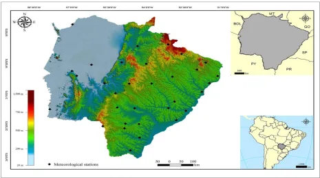
The rainfall data from 32 sites were obtained from the database of the National Water Agency - ANA, collected in the period from 1954 to 2013 (Figure 1). At each site and year, daily data were added, obtaining the monthly rainfall (mm month-1). These data were added to obtain an annual rainfall (mm year-1). Thus, were formed 32 series (localities) with different number of years of observations in each locality, defined according to the availability of the meteorological data. It was carried out the treatment and organization of precipitation data from 32 localities of the State. Historical series with faults were filled by the climatologic monthly average for each month.

Figure 1. Altimetry map (m) and representation of the meteorological stations used for spatial interpolation of the

Performance evaluation of transitive theoretical mathematical models

The annual rainfall data were submitted to a descriptive analysis in order to verify some abnormality. After, was carried a geostatistic analysis to quantify the spatial dependence of the data, through an experimental semi-variogram estimated by Equation 1.











N(h) 1 i i

i

)

Z(x

h)]²

[Z(x

2N(h)

1

γ(h)

(1)

where:

γ(h) – experimental semi-variance at distance interval h; N(h) – number of sample pairs within the distance h.; xi and xi+h – sampling locations separated by a distance h;

Z(xi) and Z(xi+h) – measured values of the variables in the corresponding localities.

Spherical variogram model is what it usually explains the majority of the studied phenomena (BENAVIDES et al., 2007). In this model, the level (C + C0) and reach (a) are identified, and usually the nugget effect (C0) is small compared to this level. The model is defined as Equation 2:

a

h

0

C

C

a

h

0,5

a

h

1,5

C

C

γ(h)

1 0 3 1

0

_

_



























































(2)

Exponential model presents a less accentuated growth from source to C + C0, which can not be said that the model really reaches the C + C0 (Equation 3):

0

h

)]

ha

exp(

[1

C

C

γ(h)

1 1

0













, (3)

where d is the maximum distance at which the variogram is set.

The Gaussian model presents good continuity in variability as the points move apart. In this model, if C0 is small, the variability structure increases in a smooth way (JIAN et al., 1996), according to Equation 4:

0

h

]

)

ha

exp(

[1

C

C

γ(h)

1 2

1

0













(4)

The parameters obtained from the fit of the variograms were used to calculate the Index of Spatial Dependence (ISD) for annual rainfall, proposed by Trangmar et al. (1985) (Equation 5):

0

10

C

C

C

(%)

ISD

0 0







(5)

where:

≤ 25% corresponds to a strong spatial dependence; 25% ≤ ISD ≤ 75 a moderate spatial dependence; ≥ 75% a weak spatial dependence.

In the study, it was adopted the mathematical interpolation method OK that allows to calculate the local average, limiting the stationary domain of the average local neighborhood centered on the point to be estimated. The values of z dimension are estimated at spatial locations (xj, yj) unobserved without the need to know the stationary mean from a linear combination of values of a local sample subset (WANDERLEY et al., 2013). The condition set out in the study was the sum of the weights of OK i (xj, yj) was equal to 1 (Equation 6).

)

y

,

Z(x

)

y

,

(x

λ

)

y

,

Z(x

_{i i}

n(j) 1 i j j i j j









(6)

where:

)

y

,

Z(x

_{j j} is estimated value by kriging in the point

(x

_j

,

y

_j

)

;

)

y

,

Z(x

_{i i} is the value of sampling in the point

(x

_i

,

y

_i

)

;

Cross validation of data and choice of models

Given the experimental semi-variogram models, was held the cross validation of the data from all transitive theoretical mathematical models based on the methodology proposed in Robinson and Metternicht (2006) and Amorim et al. (2008), at which a specific station is discarded successively in performing of interpolation; Thus, it is possible to obtain the estimated value (E) for the discarded station and then compare it with the actual value of the variable (O). One of the criteria used to choose the best transitive theoretical mathematical model was the lower value Root Mean Square Error (RMSE), according to Legates and Mccabe Jr. (1999) defined by the equation 7:

j

)

E

(O

RMSE

j 1 i 2 i i









(7)

wherein,

J – number of observations; O – value observed by measuring; E – value estimated by the method.

Camargo and Sentelhas (1997) propose that, to correlate the values estimated and the observed experimentally are considered the Pearson‟s correlation coefficient among the O x E (r) and the concordance index (d). The d values range from 0 for no agreement to 1 for perfect agreement. These values were estimated according to Equation 8:



 











 













_j 1 i 2 i i j 1 i 2 i i

O

O

O

O

)

E

(O

1

d

(8)

wherein,

O

is the mean of the values observed by the measurements.

Legates and Mccabe Jr. (1999) nd Chong et al. (1982) indicate that the smaller the value of Average Absolute Error (AAE) and Average Percentage Error (APE), expressed by Equations 9 and 10, respectively, it is better the performance of the transitive theoretical mathematical model.





J

E

O

AAE

j 1 i i i









(9)





100

J

O

E

O

APE

i j 1 i i i









 (10) III.EXPERIMENTAL RESULTS

Circular and spherical models had lower nugget effect (Table 1). The nugget effect (C0) reflects the small scale variations not detected by sampling due to the presence of measurement errors (WANDERLEY et al., 2013). This allows inferring that with the use of these transitive theoretical mathematical models the data showed fewer significant errors or variations in the estimates that might impair its use.

Circular and spheric models obtained level with similar magnitudes, corroborating the results obtained by Wanderley et al. (2013) and Uliana et al. (2013), who verified that these transitive theoretical mathematical models have a good fit to data of annual rainfall of the States of Alagoas and Espírito Santo, respectively

the sample points are correlated, or in other words, the points located in an area whose radius is the range are similar to each other in relation to separated by greater distances (WANDERLEY et al., 2013). Results in similar magnitude were observed by Ávila et al. (2009), when verified that the spherical, exponential and Gaussian models fitted to the data of probable monthly rainfall to State of Minas Gerais.

Table 1. Variographic parameters (nugget effect, level and reach) and Index of Spatial Dependence (ISD) of different

transitive theoretical mathematical models evaluated for interpolation of annual rainfall (mm year-1) in the State of Mato Grosso do Sul.

Theoretical model Nugget effect

(C0)

Level

(C + C0)

Reach (a)

IDE (%)

Circular 6.07 31.95 913.15 19.00

Spherical 6.77 32.63 705.77 20.75

Exponential 7.05 31.23 594.36 22.57

Gaussiano 9.20 38.87 638.47 23.66

.

The behaviors of the reaches showed mutual influence in almost whole region, this means that the spatial distribution of mean annual rainfall in the State is governed by the same rain producers systems As this is totals accumulated precipitates in the year, common in the summer, convective systems are little significant in terms of total rainfall, not exerting significant influence on the spatial distribution of rainfall. However, the rain producers systems correspond to the Frontal Systems (FS), South Atlantic Convergence Zone: (SACZ) and High Level Cyclonic Vortices (HLCV) which are highly significant in the rainy season and accounted for the vast majority of the total rainfall; physically, are events that affect large areas simultaneously of Mato Grosso do Sul, according to Keller Filho et al. (2005).

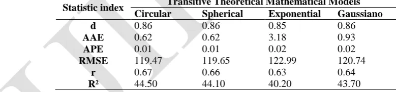
Circular, spherical and Gaussian models showed higher d, r and R² and lower AAE, APE and RMSE (Table 2), which indicates better performance for interpolation of annual rainfall of MS State. Similar results were obtained by Wanderley et al. (2013) and Uliana et al. (2013), who verified that the spherical and Gaussian models obtained better performance among those evaluated for data interpolation of annual rainfall in States of Alagoas and Espírito Santo, respectively.

Table 2. Statistic index of different transitive theoretical mathematical models evaluated for interpolation of annual

rainfall in the State of Mato Grosso do Sul.

Statistic index Transitive Theoretical Mathematical Models

Circular Spherical Exponential Gaussiano

d 0.86 0.86 0.85 0.86

AAE 0.62 0.62 3.18 0.93

APE 0.01 0.01 0.02 0.02

RMSE 119.47 119.65 122.99 120.74

r 0.67 0.66 0.63 0.64

R² 44.50 44.10 40.20 43.70

The parameter estimates of the models fitted to the semi-variograms are essential in obtaining of values not sampled by the OK methods. Values obtained by this interpolation are not addicted, have minimum variance and are ideal for building of precipitation maps, aiming to verification and interpretation of spatial variability (CASTRO et al., 2012).

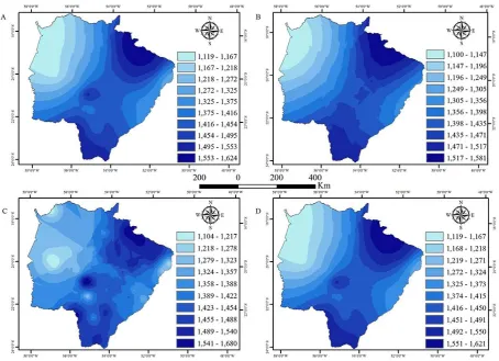
Circular, spherical and Gaussian transitive theoretical mathematical showed the same channeling pattern of the annual rainfall of the state of Mato Grosso do Sul. Comparing these models, it is observed well-defined rainfall regions, which indicated large annual variation of rainfall distribution. The results corroborate with those of Paz‑Ferreiro et al. (2010) and Castro et al. (2012), who concluded that the geostatistical approach is highly efficient in the characterization of homogeneous regions.

Figure 2. Spatial distribuitions of accumulated annual rainfall (mm year-1) in Mato Grosso do Sul, obtained by ordinary

kriging with models:Spherical (A), Gaussian (B), Exponential (C) and Circular (D).

The highest values of rainfall were observed in the south (S) and northeast (NE) of Mato Grosso do Sul. These regions operate the HLCV‟s of subtropical origin which causes rains and strong winds (CASTRO et al., 1994), the FS and SACZ. The interaction of these atmospheric systems may explain the higher means of annual rainfall.

Intermediary rainfall observed in the central region of the State by atmospheric systems of disturbed currents from the south, in the form of FS, account for 67% of the rainfall genesis in this region (KELLER FILHO et al., 2005).

IV. CONCLUSIONS

Based on different variogram and statistical index, transitive theoretical mathematical models circular, spherical and Gaussian interpolation can be used in data of annual rainfall in the State of Mato Grosso do Sul.

REFERENCES

[1]AMORIM, R. C. F., RIBEIRO, A., LEITE, C. C., LEAL, B. G. and SILVA, J. B. G., “Avaliação do desempenho de dos métodos de espacialização

da precipitação pluvial para o estado de Alagoas”, Acta Scientiarum Technology, v.30, Issue 1, pp.87-91, 2008.

[2]ÁVILA, L. F., MELLO, C. R. and VIOLA, M. R., “Mapeamento da precipitação mínima provável para o sul de Minas Gerais”, Revista Brasileira

de Engenharia Agrícola e Ambiental, v.13, pp.906-915, 2009.

[3]BARGAOUI, K. K. and CHEBBI, A., “Comparison of two kriging interpolation methods applied to spatiotemporal rainfall”, Journal of

Hydrology, v.365, pp.56-73. 2009.

[4]BENAVIDES, R. et al. “Geostatistical modelling of air temperature in a mountainous region of Northern Spain”, Agricultural and Forest

Meteorology, v.146, pp.173-188, 2007.

[5]BURROUGH, P. A. and MCDONNELL, R. A. “Principles of Geographical Information systems”, Oxford: Oxford University Press. 1998.

[6]CAMARGO, A. P. and SENTELHAS, P. C. “Avaliação do desempenho de diferentes métodos de estimativa da evapotranspiração potencial no

estado de São Paulo, Brasil” Revista Brasileira de Agrometeorologia, v.5, Issue 1, pp.89-97, 1997.

[7]CARVALHO, J. R. P. and ASSAD, E. D. “Análise espacial da precipitação pluviométrica no estado de São Paulo: Comparação de métodos de

interpolação”, Engenharia Agrícola, v.25, Issue 2, pp.377-384, 2005.

[8]CARVALHO, J. R. P., ASSAD, E. D. and PINTO, H. S., “Interpoladores geoestatísticos na análise da distribuição espacial da precipitação anual e

de sua relação com altitude”, Pesquisa Agropecuária Brasileira, v.47, Issue 9, pp.1235-1242, 2012.

[9]CASTRO, F. S., PEZZOPANE, J. E. M., CECÍLIO, R. A., PEZZOPANE, J. R. M. and XAVIER, A. C. “Avaliação do desempenho dos diferentes

métodos de interpoladores para parâmetros do balanço hídrico climatológico”, Revista Brasileira de Engenharia Agrícola e Ambiental, v.14, Issue

8, pp.871–880, 2010.

[10]CASTRO, L. H. R., MOREIRA, A. M. and ASSAD, E. D., “Definição e regionalização dos padrões pluviométricos dos cerrados brasileiros” In:

ASSAD, E.D. Chuvas nos cerrados: análise e espacialização. Brasília, Embrapa-CPAC/Embrapa-SPI, pp.423, 1994.

[11]CHILES, J. P. and DELFINER, A., “Geostatistics Modeling Spatial Uncertainty”. 1999.

[12]CHONG, S. K., GREEN, R. E. and AHUJA, L. R., “Infiltration prediction based on estimation of Green-Ampt wetting front pressure head from

measurements of soil water redistribution”, Soil Science Society of America Journal, v.46, pp.235-239, 1982.

[13]DAVIS, J. C., “Statistics and data analysis in geology”, Kansas Geological Survey. TheUniversity of Kansas, Kansas. pp.622, 2002.

[14]DEUTSCH, C. V. and JOURNEL, A. G., “GSLIB, Geostatistical Software Library and User'sGuide”, Oxford University Press, New York. 1992.

[15]GAN, W., CHEN, X., CAI, X., ZHANG, J., FENG, L. and XIE, X., “Spatial interpolation of precipitation considering geographic and topographic

influences-A case study in the Poyang Lake Watershed”, China. In: Geoscience and Remote Sensing Symposium (IGARSS), 2010 I.E. International pp. 3972–3975, IEEE, 2010.

[16]JIAN, X., OLEA, R. A. and YU, Y. S., “Semivariogram modeling by weighted least squares”, Computers & Geosciences, v.22, pp.387-397, 1996.

[17]JOURNEL, A. G. and HUIJBREGTS, C. “Mining Geostatistics”, Academic Press, New York. 1978.

[18]KEBAILI BARGAOUI, Z. and CHEBBI, A., “Comparison of two kriging interpolation methods applied to spatiotemporal rainfall”, Journal of

Hydrology, v. 365, Issue 1, pp.56-73, 2009.

[19]KELLER FILHO, T., ASSAD, E. D. and LIMA, P. R. S. R., “Regiões pluviometricamente homogêneas no Brasil”, Pesquisa Agropecuária

Brasileira, v.40, Issue 4, pp.311-322, 2005.

[20]KITANIDIS, P. K. “Introduction to Geostatistics”. University Press, Cambridge. pp.249, 1997.

[21]LEGATES, D. R. and McCABE JR, G. J., “Evaluating the use of „good-ness-of-fit‟ measures in hydrologic and hydroclimatic model validation”,

Water Resources Research, v.35, Issue 1, pp.233-241, 1999.

[22]LI, J. and HEAP, A. D., “A Review of spatial Interpolation methods for Environmental scientists”, Geoscience Australia Record 2008/23,

Cambera. Taken from the website http://www.ga.gov.au/image_cache/Ga12526.pdf on 10 September 2014. 2008.

[23]LYRA G. B., OLIVEIRA-JÚNIOR, J. F. and ZERI, M. “Cluster analysis applied to the spatial and temporal variability of monthly rainfall in Alagoas state, Northeast of Brazil”, International Journal of Climatology, v. 34, 2014.

[24]MINUZZI, R. B. and LOPEZ, R. Z., “Variabilidade de índices de chuva nos estados de Santa Catarina e Rio Grande do Sul”, Bioscience Journal, v.30, pp.697-706, 2014.

[25]NALDER, I.A. and WEIN, R.W., ”Spatial interpolation of climatic Normals: test of a new method in the Canadian boreal forest”, Agricultural and

forest meteorology 92, 211-225. 1998.

[26]OLIVEIRA-JÚNIOR, J. F., DELGADO, R. C., GOIS, G., LANNES, A., DIAS, F. O., SOUZA, J. C. S. and SOUZA, M., “Análise da Precipitação e sua Relação

com Sistemas Meteorológicos em Seropédica, Rio de Janeiro”, Floresta e Ambiente, v. 21, Issue 2, p. 140-149, 2014.

[27]PAZ‑FERREIRO, J., VIDAL VÁZQUEZ, E.V. and VIEIRA, S.R., “Geostatistical analysis of a geochemical dataset”, Bragantia, v.69,

pp.121-129, 2010.

[28]POKHREL, K. and TACHIBANA S. “A kriging method of interpolation used to map liquefaction potential over alluvial ground”, Eng Geol,

vol.152, pp.26–37. 2013.

[29]ROBINSON, T. P. and METTERNICHT, G., “Testing the performance of spatial interpolation techniques for mapping soil properties”, Computers

and Electronics in Agriculture, v.50, Issue 2, pp.97-108, 2006.

[30]SAMANTA, S., PAL, D. K., LOHAR, D. and PAL, B. “Interpolation of climate variables and temperature modeling”, Theoretical and Applied

Climatology, vol.107, 35-45. 2012.

[31]TRANGMAR, B. B., YOST, R. S. and UEHARA, G. “Application of geostatistics to special studies of soil properties”, Advance in Agronomy,

v.38, pp.45-94, 1985.

[32]ULIANA, T. M., REIS, E. F., SILVA, J. G. F. and XAVIER, A. C. “Precipitação mensal e anual provável para o Estado do Espírito Santo”, Irriga,

v.18, Issue 1, pp.139-147, 2013.

[33]VIOLA, M. R., MELLO, C. D., PINTO, D. B., MELLO, J. D. and ÁVILA, L. F., “Métodos de interpolação espacial para o mapeamento da

precipitação pluvial”, Revista Brasileira de Engenharia Agrícola e Ambiental, v.14, Issue 9, pp.970-978, 2010.

[34]WANDERLEY, H. S., AMORIM, R. F. C. and CARVALHO, F. O., “Interpolação espacial da precipitação no Estado de Alagoas utilizando

[35]WILLMOTT, C.J. “On the validation of models”, Physical Geography 2, 184-194. 1981.

[36]ISAAKS, E. H. and SRIVASTAVA, R. M., “Applied Geostatistics”, New york: Oxford University Press. 1989.

[37]YAVUZ, H. and ERDOĞAN, S., “Spatial analysis of monthly and annual precipitation trends in Turkey”, Water resources management, v. 26,

Isue 3, pp.609-621, 2012.

[38]ZAVATINI, J. A. “A dinâmica atmosférica e a distribuição das chuvas no Mato Grosso do Sul”, Tese (Doutorado) – Faculdade de Filosofia, Letras