Comparison of Compression Techniques

Volume 5, No. 1, Jan-Feb 2014

International Journal of Advanced Research in Computer Science

RESEARCH PAPER

Available Online at www.ijarcs.info

Comparison of Compression Techniques

Anitha. S Assistant Professor,

Govindammal Aditanar College for women, Tiruchendur. [email protected]

Abstract- This paper presents the various image compression techniques on the basis of analyzing existing research papers. Basically two types of image compression techniques are introduced namely lossless & lossy image compression .lossless image represented in BMP(bit map),PNG(portable network Graphics),TIFF(tagged image file format) formats and Lossy image represented in JPEG (Join photographic Experts group), JPEG 2000 formats. Lossless compression algorithms were developed to meet both the need of compression and the requirement for no change in image bits for certain applications. Video and audio files are very large unless we develop and maintain very high bandwidth networks (gigabytes per second or more) we have to compress data. Compression becomes part of the representation or coding scheme which have become popular audio,image and video formats. In the lossless group of image compression algorithms, the desire is to reduce the number of bits to represent the image in a way that is reversible without any data loss.

Index Terms- Compression, Lossless, Lossy, Compression formats, EZW, SPIHT, Huffman, PSNR.

I. INTRODUCTION

Image compression is important when it comes to storing or transmitting images. The image is an artifact that depicts or records visual perception. The idea behind image compression is to represent the image in the smallest number of bits while maintaining the essential information of the image. Compression is more or less it depends on our aim of the application . Some application require lossless reconstruction like for some medical image or satellite image application.

A. Lossless image representation formats:

a. BMP (bitmap) - is a bitmapped graphics format used internally by the Microsoft Windows graphics subsystem (GDI), and used commonly as a simple graphics file format on that platform. It is an uncompressed format.

b. PNG (Portable Network Graphics) - (1996) is a bitmap image format that employs lossless data compression. PNG was created to both improve upon and replace the GIF format with an image file format that does not require a patent license to use. It uses the DEFLATE compression algorithm, that uses a combination of the LZ77 algorithm and Huffman coding.PNG supports palette based (with a palette defined in terms of the 24 bit RGB colors), grayscale and RGB images. PNG was designed for distribution of images on the internet not for professional graphics and as such other color spaces.

c. TIFF (Tagged Image File Format) - (last review 1992) is a file format for mainly storing images, including photographs and line art. It is one of the most popular and flexible of the current public domain raster file formats. Originally created by the company Aldus, jointly with Microsoft, for use with PostScript printing, TIFF is a popular format for high color depth images, along with JPEG and

PNG. TIFF format is widely supported by image-manipulation applications, and by scanning, faxing, word processing, optical character recognition, and other applications.

B. Lossy image compression formats:

a. JPEG (Joint Photographic Experts Group) (1992) is an algorithm designed to compress images with 24 bits depth or grayscale images. It is a lossy compression algorithm. One of the characteristics that make the algorithm very flexible is that the compression rate can be adjusted. If we compress a lot, more information will be lost,but the result image size will be smaller. With a smaller compression rate we obtain a better quality, but the size of the resulting image will be bigger. This compression consists in making the coefficients in the quantization matrix bigger when we want more compression, and smaller when we want less compression.The algorithm is based in two visual effects of the human visual system. First,humans are more sensitive to the luminance than to the chrominance. Second, humans are more sensitive to changes in homogeneous areas, than in areas where there is more variation (higher frequencies). JPEG is the most used format for storing and transmitting images in Internet.

C. Summary of the formats:

II. BENEFITS OF COMPRESSION

a. It provides a believable cost savings involved with sending less data over the switched telephone network where the cost of the call is really usually based upon its duration.

b. It not only reduces storage requirements but also overall execution time.

c. It reduces the probability of transmission errors since fewer bits are transferred. 4. It provides a level of security against unlawful monitoring.

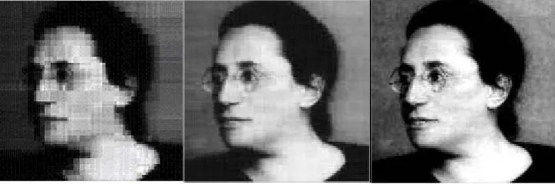
Figure 1 :This is a picture of a famous mathematician: Emmy Noether compressed in different ways

When images retrieved from the Internet, digital images take a considerable amount of time to download and use a large amount of computer memory. The Haar wavelet transform that we will discuss in this application is one way of compressing digital images so they take less space when stored and transmitted. `wavelet’’ stands for an orthogonal basis of a certain vector space.The basic idea behind this method of compression is to treat a digital image as an array of numbers i.e., a matrix. Each image consists of a fairly

large number of little squares called pixels (picture elements). The matrix corresponding to a digital image assigns a whole number to each pixel. For example, in the case of a 256x256 pixel gray scale image, the image is stored as a 256x256 matrix, with each element of the matrix being a whole number ranging from 0 (for black) to 225 (for white). The JPEG compression technique divides an image into 8x8 blocks and assigns a matrix to each block.

Figure: 2

III. IMAGE COMPRESSION TECHNIQUES

The image compression techniques are broadly classified into two categories depending whether or not an exact replica of the original image could be reconstructed using the compressed image .These are:

A. Lossless technique B. Lossy techniqhe

A. Lossless compression technique:

In lossless compression techniques, the original image can be perfectly recovered form the compressed (encoded)

image. These are also called noiseless since they do not add noise to the signal (image).It is also known as entropy coding since it use statistics/decomposition techniques to eliminate/minimize redundancy. Lossless compression is used only for a few applications with stringent requirements such as medical imaging. Following techniques are included in lossless compression:

B. Lossy compression technique:

Lossy schemes provide much higher compression ratios than lossless schemes. Lossy schemes are widely used since the quality of the reconstructed images is adequate for most applications .By this scheme, the decompressed image is not identical to the original image, but reasonably close to it.

IV. LOSSLESS COMPRESSION TECHNIQUES

A. Run Length Encoding:

This encoding method is frequently applied to images (or pixels in a scan line). It is a small compression component used in JPEG compression. It is useful in case of repetitive data. This technique replaces sequences of identical symbols (pixels) ,called runs by shorter symbols. For example:

Original Sequence:

111122233333311112222 can be encoded as:

(1,4),(2,3),(3,6),(1,4),(2,4)

B. Huffman Encoding:

Huffman coding is based on the frequency of occurrence of a data item (pixel in images). The principle is to use a lower number of bits to encode the data that occurs more frequently. Codes are stored in a Code Book which may be constructed for each image or a set of images. In all cases the code book plus encoded data must be transmitted to enable decoding. This is a general technique for coding symbols based on their statistical occurrence frequencies (probabilities). The pixels in the image are treated as symbols. Huffman coding and the like use an integer number (k) of bits for each symbol, hence k is never less than 1. Sometimes, e.g., when sending a 1-bit image, compression becomes impossible. Huffman code is a prefix code. This means that the (binary) code of any symbol is not the prefix of the code of any other symbol. Most image coding standards use lossy techniques in the earlier stages of compression and use Huffman coding as the final step.

C. LZW Coding:

a. LZW (Lempel- Ziv – Welch ) methods due to Ziv and Lempel in 1977 and 1978. Terry Welch improved the scheme in 1984 (called LZW compression).

b. It is a dictionary based coding.Dictionary based coding can be static or dynamic. In static dictionary coding, dictionary is fixed during the encoding and decoding processes. In dynamic dictionary coding, the dictionary is updated on fly.

c. It is used in UNIX compress -1D token stream (similar to below)

d. It used in GIF compression - 2D window tokens (treat image as with Huffman Coding Above).

D. Area Coding :

Area coding is an enhanced form of run length coding, reflecting the two dimensional character of images. This is a significant advance over the other lossless methods.

E. Lossy compression Techniques:

Lossy compression as the name implies leads to loss of some information. The compressed image is similar to the original uncompressed image but not just like the previous as in the process of compression some information

concerning the image has been lost. They are typically suited to images. The most common example of lossy compression is JPEG. An algorithm that restores the presentation to be the same as the original image are known as lossy techniques. Reconstruction of the image is an approximation of the original image, therefore the need of measuring of the quality of the image for lossy compression technique. Lossy compression technique provides a higher compression ratio than lossless compression. Major performance considerations of a lossy compression scheme include:

a) Compression ratio b) Signal to noise ratio

c) Speed of encoding & decoding

F. Lossy image compression techniques include following schemes:

a. Scalar Quantization: The most common type of quantization is known as scalar quantization. Scalar quantization, typically denoted as Y=Q (x), is the process of using a quantization function Q to map a scalar (one-dimensional) input value x to a scalar output value Y [1]. Scalar quantization can be as simple and intuitive as rounding high-precision numbers to the nearest integer, or to the nearest multiple of some other unit of precision.

b. Vector Quantization: Vector quantization (VQ) is a classical quantization technique from signal processing which allows the modeling of probability density functions by the distribution of prototype vectors. It was originally used for image compression . It works by dividing a large set of points (vectors) into groups having approximately the same number of points closest to them. The density matching property of vector quantization is powerful, especially for identifying the density of large and high-dimensioned data. Since data points are represented by the index of their closest centroid, commonly occurring data have low error, and rare data high error. This is why VQ is suitable for lossy data compression. It can also be used for lossy data correction and density estimation.

V. LITERATURE SURVAY

In 2010, Jau-Ji Shen et al presents vector quantization based image compression technique [2]. In this paper they adjust the encoding of the difference map between the original image and after that it’s restored in VQ compressed version. Its experimental results show that although there scheme needs to provide extra data, it can substantially improve the quality of VQ compressed images, and further be adjusted depending on the difference map from the lossy compression to lossless compression.

for compression that provides good compression efficiency and has lower computational complexity as compared to the standard SPIHT technique for lossless compression.

In 2012, Firas A. Jassim, et al presents a novel method for image compression which is called five module method (FMM). In this method converting each pixel value in 8x8 blocks [4] into a multiple of 5 for each of RGB array. After that the value could be divided by 5 to get new values which are bit length for each pixel and it is less in storage space than the original values which is 8 bits. This paper demonstrates the potential of the FMM based image compression techniques. The advantage of their method is it provided high PSNR (peak signal to noise ratio) although it is low CR (compression ratio). This method is appropriate for bi-level like black and white medical images where the pixel in such images is presented by one byte (8 bit). As a recommendation, a variable module method (X) MM, where X can be any number, may be constructed in latter research.

In 2012, Ashutosh Dwivedi, et al presents a novel hybrid image compression technique. This technique inherits the properties of localizing the global spatial and frequency correlation from wavelets and classification and function approximation tasks from modified forward-only counter propagation neural network (MFOCPN) for image compression. In this scheme several tests are used to investigate the usefulness of the proposed scheme. In this paper, they explore the use of MFO-CPN [5] networks to predict wavelet coefficients for image compression. In this method, they combined the classical wavelet based method with MFO-CPN. The performance of the proposed network is tested for three discrete wavelet transform functions. In this they analysis that Haar wavelet results in higher compression ratio but the quality of the reconstructed image is not good. On the other hand db6 with the same number of wavelet coefficients leads to higher compression ratio with good quality. Overall they found that the application of db6 wavelet in image compression out performs other two.

In 2012, Yi-Fei Tan, et al presents image compression technique based on utilizing reference points coding with threshold values. This paper intends to bring forward an image compression method which is capable to perform both lossy and lossless compression. A threshold [6] value is associated in the compression process, different compression ratios can be achieved by varying the threshold values and lossless compression is performed if the threshold value is set to zero. The proposed method allows the quality of the decompressed image to be determined during the compression process. In this method If the threshold value of a parameter in the proposed method is set to 0, then lossless compression is performed. Lossy compression is achieved when the threshold value of a parameter assumes positive values. Further study can be performed to calculate the optimal threshold value T that should be used.

In 2012, S.Sahami, et al presents a bi-level image compression techniques using neural networks. It is the lossy image compression technique. In this method, the locations of pixels of the image are applied to the input of a multilayer perceptron neural network [7]. The output the network denotes the pixel intensity 0 or 1. The final weights of the trained neural-network are quantized, represented by few bites, Huffman encoded and then stored as the compressed image. Huffman encoded and then stored as the

compressed image. In the decompression phase, by applying the pixel locations to the trained network, the output determines the intensity. The results of experiments on more than 4000 different images indicate higher compression rate of the proposed structure compared with the commonly used methods such as comite consultatif international telephonique of telegraphique graphique (CCITT) G4 and joint bi-level image expert group (JBIG2) standards. The results of this technique provide High compression ratios as well as high PSNRs were obtained using the proposed method. In the future they will use activity, pattern based criteria and some complexity measures to adaptively obtain high compression rate.

In 2013, C. Rengarajaswamy, et al presents a novel technique in which done encryption and compression of an image. In this method stream cipher is used for encryption of an image after that SPIHT [8] is used for image compression. In this paper stream cipher encryption is carried out to provide better encryption used. SPIHT compression provides better compression as the size of the larger images can be chosen and can be decompressed with the minimal or no loss in the original image. Thus high and confidential encryption and the best compression rate has been energized to provide better security the main scope or aspiration of this paper is achieved. In 2013, S. Srikanth, et al presents a technique for image compression which is use different embedded Wavelet based image coding with Huffman-encoder for further compression. In this paper they implemented the SPIHT and EZW algorithms with Huffman encoding [9] using different wavelet families and after that compare the PSNRs and bit rates of these families. These algorithms were tested on different images, and it is seen that the results obtained by these algorithms have good quality and it provides high compression ratio as compared to the previous exist lossless image compression techniques.

In 2013, Pralhadrao V Shantagiri, et al presents a new spatial domain of lossless image compression algorithm for synthetic color image of 24 bits. This proposed algorithm use reduction of size of pixels for the compression of an image. In this the size of pixels [10] is reduced by representing pixel using the only required number of bits instead of 8 bits per color. This proposed algorithm has been applied on asset of test images and the result obtained after applying algorithm is encouraging. In this paper they also compared to Huffman, TIFF, PPM-tree, and GPPM. In this paper, they introduce the principles of PSR (Pixel Size Reduction) lossless image compression algorithm. They also had shows the procedures of compression and decompression of their proposed algorithm. Future work of this paper uses the other tree based lossless image compression algorithm.

used for the lossless image compression. The bit rate obtained using the MS-VLI (Magnitude Set-Variable Length Integer Representation) with RLE scheme is about 2.1 bpp (bits per pixel) to 3.1 bpp less then that obtain using MS-VLI without RLE scheme.

In 2013 S. Dharanidharan, et al presents a new modified international data encryption algorithm to encrypt the full image in an efficient secure manner [12] , and encryption after the original file will be segmented and converted to other image file. By using Huffman algorithm the segmented image files are merged and they merge the entire segmented image to compress into a single image. Finally they retrieve a fully decrypted image. Next they find an efficient way to transfer the encrypted images to multipath routing techniques. The above compressed image has been sent to the single pathway and now they enhanced with the multipath routing algorithm, finally they get an efficient transmission and reliable, efficient image.

VI. DIFFERENTTYPESOFIMAGE

COMPRESSIONALGORITHMS

The various types of image compression methods are described below:

A. Embedded zero wavelet coding {EZW}:

The EZW algorithm was one of the first algorithms to show the full power of wavelet-based image compression. It was introduced in the groundbreak ing paper of Shapiro . We shall describe EZW in some detail because a solid understanding of it will make it much easier to comprehend the other algorithms we shall be discussing. These other algorithms build upon the fundamental concepts that were first introduced with EZW.Our discussion of EZW will be focused on the fundamental ideas underly ing it; we shall not use it to compress any images. That is because it has been superseded by a far superior algorithm, the SPIHT algorithm. Since SPIHT is just a highly refined version of EZW, it makes sense to first describe EZW. EZW stands for Embedded Zerotree Wavelet. We shall explain the terms Embedded, and Zerotree, and how they relate to Wavelet-based compression. An embedded coding is a process of encoding the transform magnitudes that allows for progressive transmission of the compressed image. Zerotrees are a concept that allows for a concise encoding of the positions of significant values that result during the embedded coding process. We shall first discuss embedded coding, and then examine the notion of zerotrees. The embedding process used by EZW is called bit-plane encoding.

B. Set Partitioning in Hierarchical Trees (SPIHT): SPIHT is the wavelet based image compression method. It provides the Highest Image Quality, Progressive image transmission, fully embedded coded file, Simple quantization algorithm, fast coding/decoding, completely adaptive, Lossless compression, Exact bit rate coding and Error protection. SPIHT makes use of three lists – the List of Significant Pixels (LSP), List of Insignificant Pixels (LIP) and List of Insignificant Sets (LIS). These are coefficient location lists that contain their coordinates. After the initialization, the algorithm takes two stages for each level of threshold – the sorting pass (in which lists are organized) and the refinement pass (which does the actual progressive

coding transmission). The result is in the form of a bit stream. It is capable of recovering the image perfectly (every single bit of it) by coding all bits of the transform. However, the wavelet transform yields perfect reconstruction only if its numbers are stored as infinite imprecision numbers. Peak signalto noise ratio (PSNR) is one of the quantitative measures for image quality evaluation which is based on the mean square error (MSE) of the reconstructed image. The MSE for K x M size image is given by:

MSE=1/MK

Where f(i,j) is the original image data and f1(i,j) is the compressed image value. The formula for PSNR is calculated by

PSNR=10 log((255)2/ MSE )

C. Spiht coding algorithm:

Since the order in which the subsets are tested for significance is important in a practical implementation the significance information is stored in three ordered lists called list of insignificant sets (LIS) list of insignificant pixels (LIP) and list of significant pixels (LSP). In all lists each entry is identified by a coordinate (i, j) which in the LIP and LSP represents individual pixels and in the LIS represents either the set D (i, j) or L (i, j) . To differen tiate between them it can be concluded that a LIS entry is of type A if it represents D (i,j) and of type B if it represents L(i, j). During the sorting pass the pixels in the LIP-which were insignificant in the previous pass-are tested and those that become significant are moved to the LSP. Similarly, sets are sequentially evaluated following the LIS order, and when a set is found to be significant it is removed from the list and partitioned. The new subsets with more than one element are added back to the LIS, while the single coordinate sets are added to the end of the LIP or the LSP depending whether they are insignificant or significant respectively. The LSP contains the coordinates of the pixels that are visited in the refinement pass. Below the new encoding algorithm in presented.

D. Huffman encoding:

represent four characters. And so on. Unlike ASCII code, which is a fixed length code using seven bits per character, Huffman encoding compression is a variable length coding system that assigns smaller codes for more frequently used characters and larger codes for less frequently used characters in order to reduce the size of files being compressed and transferred.The decoding algorithm is just the reverse of the coding algorithm. But a difference with coding algorithm is that the LIP and LSP are stored as co-ordinates and the LIS stores only the pixel coco-ordinates of the topmost modes of the descendent trees and does not store VTs. Because during the decoding, testing whether a descendent tree is significant or not requires only whether the corresponding bit is 1 or zero, it does not require exhaustive searching as in the case of coding. In other words decoding remains the same as in SPIHT except the way of representation of the tree structure.

VII. TERMSUSEDINIMAGECOMPRESSION

There are various types of terms that are used in calculation of image compression. Some are listed below:

A. Peak signal to noise ratio:

The phrase peak signal-to-noise ratio, often abbreviated PSNR, is an engineering term for the ratio between the maximum possible power of a signal and the power of corrupting noise that affects the fidelity of its representation. Because many signals have a very wide dynamic range, PSNR is usually expressed in terms of the logarithmic decibel scale. The PSNR is most commonly used as a measure of quality of reconstruction in image compression etc. It is most easily defined via the mean squared error (MSE) which for two m×n monochrome images I and K

where one of the images is considered a noisy approximation of the other is defined as:

MSE=1/MK

The PSNR is defined as:

PSNR=10 *log ((MAX ) MSE) 20*log10 {MAX1/sqrt[MSE]} Here, MAXi is the maximum possible pixel value of the image. When the pixels are represented using 8 bits per sample, this is 255. More generally, when samples are represented using linear PCM with B bits per sample, MAXI is 2 B-1 For color images with three RGB values per pixel, the definition of PSNR is the same except the MSE is the sum over all squared value differences divided by image size and by three. An identical image to the original will yield an undefined PSNR as the MSE will become equal to zero due to no error. In this case the PSNR value can be thought of as approaching infinity as the MSE approaches zero; this shows that a higher PSNR value provides a higher image quality. At the other end of the scale an image that comes out with all zero value pixels (black) compared to an original does not provide a PSNR of zero . This can be seen by observing the form, once again, of the MSE equation. Not all the original values will be a long distance from the zero value thus the PSNR of the image with all pixels at a value of zero is not the worst possible case.

B. Signal-to-noise ratio:

It is an electrical engineering concept, also used in other fields (such as scientific measurements, biological cell

signaling), defined as the ratio of a signal power to the noise power corrupting the signal. In less technical terms, signal-to-noise ratio compares the level of a desired signal (such as music) to the level of background noise . The higher the ratio, the less obtrusive the background noise is. In engineering, signal-to-noise ratio is a term for the power ratio between a signal (meaningful information) and the background noise:

SNR=Psignal/ PNoise=[ASignal/ANoise]2

Where P is average power and A is RMS amplitude. Both signal and noise power (or amplitude) must be measured at the same or equivalent points in a system, and within the same system bandwidth. Because many signals have a very wide dynamic range, SNRs are usually expressed in terms of the logarithmic decibel scale. In decibels, the SNR is, by definition, 10 times the logarithm of the power ratio. If the signal and the noise is measured across the same impedance then the SNR can be obtained by calculating 20 times the base-10 logarithm of the amplitude ratio:

SNR=10*log10(Psignal/PNoise)=20*log10 =[ASignal/ANoise]2

In image processing, the SNR of an image is usually defined as the ratio of the mean pixel value to the standard deviation of the pixel values. Related measures are the "contrast ratio" and the "contrast-tonoise

ratio". The Rose criterion (named after Albert Rose) states that an SNR of at least 5 is needed to be able to distinguish image features at 100% certainty. An SNR less than 5 means less than 100% certainty in identifying image details.

C. Mean Square Error:

In statistics, the mean square error or MSE of an estimator is one of many ways to quantify the amount by which an estimator differs from the true value of the quantity being estimated. As a loss function MSE is called squared error loss. MSE measures the average of the square of the "error". The error is the amount by which the estimator differs from the quantity to be estimated. The difference occurs because of randomness or because the estimator doesn't account for information that could produce a more accurate estimate. The MSE is the second moment (about the origin) of the error, and thus incorporates both the variance of the estimator and its bias. For an unbiased estimator, the MSE is the variance. Like the variance, MSE has the same unit of measurement as the square of the quantity being estimated. In an analogy to standard deviation, taking the square root of MSE yields the root mean square error or RMSE, which has the same units as the quantity being estimated; for an unbiased estimator, the RMSE is the square root of the variance, known as the standard error. Definition and basic properties The MSE of an estimator θ1 with respect to the estimated parameter θis defined as

MSE(θ1)= E((θ1 - θ)2 )

The MSE can be written as the sum of the variance and the squared bias of the estimator

MSE(θ1) =Var(θ1)+ (Bias(θ1, θ))2

MSE(θ1)=1 (θj -θ)2

VIII. EXPERIMENTAL RESULTS

A. PSNR comparison:

Computational formula of PSNR and mean square error (MSE).

PSNR= 10* lg[(2n-1)2/MSE]

MSE= /(M*K)

Firstly, original image is applied to the compression program, EZW encoded image is obtained. To reconstruct

compressed image, compressed image is applied to decompression program, by which EZW decoded image is obtained. Compression Ratio (CR) and Peak-Signal-to-Noise Ratio (PSNR) are obtained for the original and reconstructed images. In the experiment the original image ‘Cameraman.tif’ having size 256 x 256 (65,536 Bytes). The different statistical values of the image cameraman.tif for Various Thresholds are summarized in the table. Thus, it can be concluded that EZW encoding gives excellent results. By choosing suitable threshold value compression ratio as high as 8 can be achieved

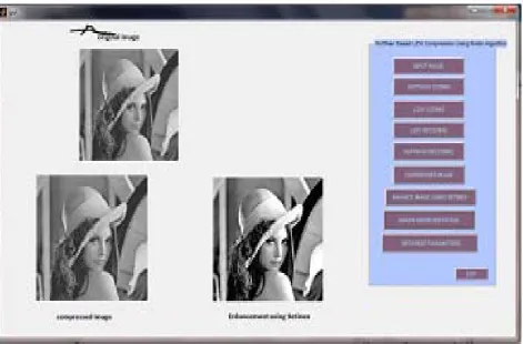
Figure 2 Graphical User Interface of Huffman Based LZW Lossless Image Compression using Retinex Algorithm

The experiment results are shown below.

Figure 3 Perform Huffman Based LZW Compression using Retinex algorithm on house image

Table 2

Images Compression Ratio

PSNR MSE

Lena 6.23 48.06 1.87

House 5.45 47.30 1.65

Graphical Representation of Images Based on Different Quality Metrics using Huffman Based LZW Lossless Image Compression using Retinex Algorithm

IX. CONCLUSION

applications like security technologies. After study of all techniques it is found that lossless image compression techniques are most effective over the lossy compression techniques. Lossy provides a higher compression ratio than lossless.

X. REFERENCES

[1]. Gaurav vijayvargiya,Dr.sanjay silakari,Dr.Rajeev pandey ,A survey various techniques of image compression-IJCSIS vol1.11,No.!0 .Oct 2013

[2]. Jau-Ji Shen and Hsiu-Chuan Huang,‖ An Adaptive Image Compression Method Based on Vector Quantization,‖IEEE, pp. 377-381, 2010.

[3]. Suresh Yerva, Smita Nair and Krishnan Kutty,‖ Lossless Image Compression based on Data Folding,‖IEEE, pp. 999-1004, 2011.

[4]. Firas A. Jassim and Hind E. Qassim,‖ F ive Modulus Method for Image Compression,‖ SIPIJ Vol.3, No.5, pp. 19-28, 2012.

[5]. Mridul Kumar Mathur, Seema Loonker and Dr. Dheeraj

Saxena ―Lossless Huffman Coding Technique For Image

Compression And Reconstruction Using Binary Trees,

‖IJCTA, pp. 76-79, 2012.

[6]. V.K Padmaja and Dr. B. Chandrasekhar,‖Literature Review of Image Compression Algorithm,‖ IJSER, Volume 3, pp. 1-6, 2012.

[7]. Jagadish H. Pujar and Lohit M. Kadlaskar,‖ A New Lossless Method Of Image Compression and

Decompression Using Huffman Coding Techniques,‖ JATIT, pp. 18-22, 2012.

[8]. Ashutosh Dwivedi, N Subhash Chandra Bose, Ashiwani Kumar,‖A Novel Hybrid Image Compression Technique: Wavelet-MFOCPN‖pp. 492-495, 2012.

[9]. Yi-Fei Tan and Wooi-Nee Tan,‖ Image Compression Technique Utilizing Reference Points Coding with Threshold Values,‖IEEE, pp. 74-77, 2012.

[10]. S. Sahami and M.G. Shayesteh,‖ Bi -level image compression technique using neural networks,‖ IET Image Process, Vol. 6, Iss. 5, pp. 496–506, 2012.

[11]. C. Rengarajaswamy and S. Imaculate Rosaline,‖ SPIHT Compression of Encrypted Images,‖IEEE, pp. 336 -341,2013.

[12]. S.Srikanth and Sukadev Meher,‖ Compression Efficiency for Combining Different Embedded Image Compression Techniques with Huffman Encoding,‖IEEE, pp. 816 -820, 2013.

[13]. Compression Efficiency for combing different embedded image compression techniques with Huffman encoding-Thesis submitted by sure srikanth.

Short Bio Data for the Author