Improvement of Apriori Algorithm by Reducing Number of Database Scans and Generation of Candidate Keys

(1)

Volume 7, No. 2, March-April 2016

International Journal of Advanced Research in Computer Science

RESEARCH PAPER

Available Online at www.ijarcs.info

Improvement of Apriori Algorithm by Reducing Number of Database Scans and

Generation of Candidate Keys

Anneshya Ghosh

Department of Computer Science

Birla Institute of Technology, Mesra, Kolkata Campus Kolkata, India

Ambar Dutta

Department of Computer Science

Birla Institute of Technology, Mesra, Kolkata Campus Kolkata, India

Abstract: Finding frequent itemsets is a key step in various data mining applications to find interesting patterns from databases. Association rule mining is an important technique in data mining. Apriori algorithm is most basic, simplest and classical algorithm of association rule mining. This algorithm is considered as an efficient algorithm, but still it has some drawbacks. In the literature, there exist a number of improvements for mining association rules based on Apriori algorithm. According to the problem that the traditional Apriori algorithm needs to scan database frequently, an improved strategy and corresponding algorithm is put forward in this paper. A comparative study of the traditional Apriori, existing improvements and proposed improved version of Apriori algorithm is presented in this paper with the help of different databases.

Keywords: Data Mining; Apriori algorithm; Support; Database; Frequent Itemsets.

I. INTRODUCTION

Data Mining [1] is a process where information or knowledge is being extracted or mined from a large set of dataset. Here the sequential patterns that are present in the large databases are mined. Sequential Pattern Mining was first introduced by Agarwal and Srikant in the year 1994. Sequence patterns are those set of data which occurs in a specific order that is sequentially, out of all the data patterns in a given set. And finding out of these patterns which occurs sequentially out of all the other patterns is Sequential Pattern Mining. An example of sequential pattern is as follows; suppose a customer buys a laptop then the customer will buy a mouse then an antivirus and a printer following it sequentially. Some terms which are constantly being used here are item-set, support and confidence. Let there be a set of items L = {l1, l2 …}, a sub set of these items is knows as item-set. For a given database D, support of an item, let be X, is defined as the ratio of the number of sequences in the database which contain the item X to the total number of sequences that are present in the database. And, for a given database D, confidence of a sequence that contains X as well as Y is defined as the percentage of the number of sequences that contains X as well as Y to the total number of sequences which contains X.

Mining of sequential patterns can be classified into three different categories, they are as 1. Mining based on candidate generation (example, Apriori algorithm), 2. Mining without the involvement of any candidate generation (example, FP-Growth Tree algorithm) and 3. Mining item sets which have vertical format (example, ECLAT algorithm).Apriori algorithm is the algorithm which involves Candidate generation. According to this algorithm, first the 1-itemsets are found then the database is scanned to find the support count. The itemsets with support count less than minimum support count are discarded. The resultant itemsets are then used to find the frequent 2-itemsets in the same process. Likewise we find all the (k+1)-itemsets from the frequent k-itemsets, until no more frequent itemsets can be found out. In FP-Growth tree algorithm [2], candidate keys are not generated and database is scanned for two times only. It uses a tree like structure to store the database and uses a

divide and conquer method. And in ECLAT algorithm [2], depth first search method is used. During the first scan of the database, a Transcation Id (TID) list is provided to each single item. It is followed by the generation of (k+1) itemsets from the k itemsets using apriori property and depth first search method by taking the intersection of the TID - set of frequent k-itemsets. This process is continued, until no more candidates itemset can be found.

In this paper, Apriori algorithm is taken into consideration. In the next section, section II, Apriori algorithm is discussed in details. In section III, some of the existing improved algorithms are discussed with examples. Then in section IV, the proposed improved Apriori algorithm is discussed. In section V comparisons between the original, existing and the proposed improved Apriori algorithm is shown. Finally conclusion is drawn in section VI.

II. APRIORI ALGORITHM

A. Description

The first and the most basic algorithm which was developed to find out the sequential patterns from a database was the Apriori algorithm [3]. This algorithm involves candidate generation and was first proposed by R. Agarwal and R. Srikant in the year 1994. In Apriori algorithm, the original database is first scanned and the support count of each of the individual items is found out. And those items whose support count is less than the minimum support count are discarded. The resultant item set is then used to find out the frequent 2-items set. From where again support count of each item-set is calculated and only those items whose support count is more than minimum support count are kept and others are discarded. Next we find out the frequent 3-item set and then frequent 4-item set, till no more frequent 4-item sets can be generated. The final frequent item set which is generated and satisfies the minimum support count is our final frequent pattern.

Table I. Original Database

(2)

1 T1 ABD

2 T2 ABCD

3 T3 ABE

4 T4 BEF

5 T5 ABDF

6 T6 AE

7 T7 C

[image:2.595.93.238.58.165.2]

8 T8 EF

Table II. Support Count (Minimum Support Count=2)

Table III. Frequent 2-Item Set

Table IV. Frequent 3-Itemset

Sr. No. Items Support

Count

1 ABD 3

2 ABE 1 (X)

3 ABF 1 (X)

4 ADE 0 (X)

5 AEF 0 (X)

6 BDE 0 (X)

7 BDF 1 (X)

8 BEF 1 (X)

Total number for scans required for finding out the frequent 1-itemset = 6x8 = 48.

Total number of scans required for finding out the frequent 2-itemsets = 15x8 = 120.

Total number of scans required for finding out the frequent 3-itemsets = 8x8 = 64.

B. Limitations

The advantage of Apriori algorithm is that it is a simple algorithm and can be implemented easily. But it still has some disadvantages also. The main disadvantage is that here the entire database needs to be scanned at each step. Also in this algorithm, a large number of candidate keys are generates. And if the database is very large than scanning in each step not only consumes a lot of time but the generation of a large number candidate keys consumes a lot of memory also, which can be sometimes limited. Therefore this algorithm can work well for small database but not for large database.

III. EXISTING IMPROVED APRIORI ALGORITHMS

A number of improvements for Apriori algorithm have been proposed to overcome the limitations of the algorithm. In this section we will discuss some of the improvements and compare them. We will take into consideration those improvements which will reduce the number of scans and also the number of candidate key generation.

A. Algorithm for reducing the number of scan (Algorithm 1)

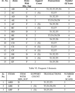
[image:2.595.83.233.181.680.2]

In this algorithm [4], Apriori algorithm is improved by reducing the number of scans. In this algorithm the first step is same as the classical Apriori algorithm. But in the second step, from each of the frequent 2-item set the one with minimum support count is first found out and then the transactions where that item is present. Next only from that transaction the frequent 2-items set are checked and the support count of individual set are found out. For all the next frequent item set the same process is followed. In this the number of scans gets reduced. The algorithm works as shown in Table II, Table V and Table VI.

Table V. Frequent 2-Itemsets

Sr. No. Items Items

With Min_Sup

Support Count

Transactions Number

Of Scans

1 AB A 4 T1,T2,T3,T5,T6 5

2 AC C 1 (X) T2,T7 2

3 AD D 3 T1,T2,T5 3

4 AE E 2 T3,T4,T6,T8 4

5 AF F 1 (X) T4,T5,T8 3

6 BC C 1 (X) T2,T7 2

7 BD D 3 T1,T2,T5 3

8 BE E 2 T3,T4,T6,T8 4

9 BF F 2 T4,T5,T8 3

10 CD C 1 (X) T2,T7 2

11 CE C 0 (X) T2,T7 2

12 CF C 0 (X) T2,T7 2

13 DE D 0 (X) T1,T2,T5 3

14 DF D 1 (X) T1,T2,T5 3

15 EF F 2 T4,T5,T8 3

Table VI. Frequent 3-Itemsets

Sr. No.

ITEMS ITEM WITH MIN_SUP

SUPPORT COUNT

TRANSACTIONS NUMBER OF SCANS

1 ABD D 3 T1,T2,T5 3

2 ABE E 1 (X) T3,T4,T6,T8 4

3 ABF F 1 (X) T4,T5,T8 3

1 A 5

2 B 5

3 C 2

4 D 3

5 E 4

6 F 3

Count

1 AB 4

2 AC 1 (X)

3 AD 3

4 AE 2

5 AF 1 (X)

6 BC 1 (X)

7 BD 3

8 BE 2

9 BF 2

10 CD 1 (X)

11 CE 0 (X)

12 CF 0 (X)

13 DE 0 (X)

14 DF 1 (X)

[image:2.595.301.565.461.786.2]

(3)

4 ADE D 0 (X) T1,T2,T5 3

5 AEF F 0 (X) T4,T5,T8 3

6 BDE D 0 (X) T1,T2,T5 3

7 BDF D 1 (X) T1,T2,T5 3

8 BEF F 1 (X) T4,T5,T8 3

Number of scans required for finding out frequent 2-itemsets = (5+2+3+4+3+2+3+4+3+2+2+2+3+3+3) = 44.

Number of scans required for finding out the frequent 3-itemsets = (3+4+3+3+3+3+3+3) = 25.

B. Algorithm for reducing database size and number of scans (Algorithm 2)

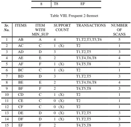
In this algorithm [5], Apriori algorithm was improved by both reducing the number of scans as well as cutting down the size of the database and removing some transactions which are not required. As a result the search time gets reduced by two times. In this algorithm also the first step is same as the original Apriori algorithm. And the for frequent 2-item set, all the transactions from the database which has less than 2 items are first deleted, then for each individual 2-item sets, the item with the minimum support among the two are first found and for the 2-ietms sets only in those transactions where the minimum support items are present are searched and their support count are calculated. Those item-sets which support count less than the minimum support count are removed. From the resultant set we find frequent 3-item set and so on. The algorithm is illustrated by Table II, Table VII, Table VIII, Table IX and Table X.

Table VII. Reduced Database For Frequent 2-Itemset

Sr. No. Transaction Items

1 T1 ABD

2 T2 ABCD

3 T3 ABE

4 T4 BEF

5 T5 ABDF

6 T6 AE

7 T7 C (X)

[image:3.595.28.297.516.776.2]

8 T8 EF

Table VIII. Frequent 2-Itemset

Sr. No.

SUPPORT COUNT

1 AB A 4 T1,T2,T3,T5,T6 5

2 AC C 1 (X) T2 1

3 AD D 3 T1,T2,T5 3

4 AE E 2 T3,T4,T6,T8 4

5 AF F 1 (X) T4,T5,T8 3

6 BC C 1 (X) T2 1

7 BD D 3 T1,T2,T5 3

8 BE E 2 T3,T4,T6,T8 4

9 BF F 2 T4,T5,T8 3

10 CD C 1 (X) T2 1

11 CE C 0 (X) T2 1

12 CF C 0 (X) T2 1

13 DE D 0 (X) T1,T2,T5 3

14 DF D 1 (X) T1,T2,T5 3

15 EF F 2 T4,T5,T8 3

Table IX. Reduced Table for Frequent 3-I

1 T1 ABD

2 T2 ABCD

3 T3 ABE

4 T4 BEF

5 T5 ABDF

6 T6 AE (X)

7 T7 C (X)

8 T8 EF (X)

Table X. Frequent 3-Itemset

Sr. No.

SUPPORT COUNT

1 ABD D 3 T1,T2,T5 3

2 ABE E 1 (X) T3,T4 2

3 ABF F 1 (X) T4,T5 2

4 ADE D 0 (X) T1,T2,T5 3

5 AEF F 0 (X) T4,T5 2

6 BDE D 0 (X) T1,T2,T5 3

7 BDF D 1 (X) T1,T2,T5 3

8 BEF F 1 (X) T4,T5 2

Number of scans required for finding out the 2-itemset = (5+1+3+4+3+1+3+4+3+1+1+1+3+3+3) = 39.

Number of scans required for finding out the 3-itemset = (3+2+2+3+2+3+3+2) =20.

C. Transaction Reduction and Matrix Method (Algorithm 3)

In this proposed algorithm [6], items (In) and transactions

(Tm) from the database are mapped into a matrix with size

mXn. In this matrix, transactions are represented by the rows and the items are represented by the columns. The elements on this matrix are either 0 or 1 and is decides as follows:

Martix = [aij] = 1, if in transaction i there is item j, and

Matrix = [aij] = 0, otherwise.

(4)

[image:4.595.40.242.66.184.2]

Figure 1. Frequent 1-itemsets.

[image:4.595.36.264.223.360.2]

Number of scans required for 1-itemset = 6X8 = 48.

Number of scans required for 2-itemset = 15X8 =120.

Number of scans required for 3-itemset =8X5 = 40.

IV. PROPOSED ALGORITHM

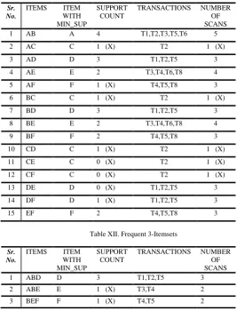
In our proposed algorithm, the database size, the number of database scans as well as the number of candidate keys generated is reduced. For finding each (k+1) frequent itemset all the items from the database that have number of items less than (k+1) are removed. And secondly, according to the algorithm, the database for those k-frequent itemsets whose number of transaction is less than minimum support is not scanned. This 2 steps will reduce the number of database scans. And for candidate key generation, only those (k+1) itemset whose individual pair are present in frequent k-itemset is consider. This will reduce the number of candidate key generation and also unnecessary scan of the database.

A. The algorithm

1. First, 1-itemset from the database is found out.

Repeat step 2-7, until no more frequent patterns can be found out.

2. The support count of them is calculated by scanning the database. Those item whose support count is less than the minimum support count are removed.

3. Before finding out (k+1)-itemsets, all the transaction from the database which have number of items less than k are removed.

4. Then the join operation of the frequent k-itemset is performd to find out the (k+1)-itemset.

5. For finding out (k+1)-itemsets each pair of k-itemsets are first checked whether are frequent or not. If all the individual k-itemsets are frequent then only that particular (k+1)itemset is considered frequent.

6. For each (k+1) itemset, the item with the minimum support count among each of the (k+1) items is first found out and then the transactions where that item is present. Only those transactions are then scanned for that particular (k+1) items in the whole database.

7. Now, if the number of transactions found out is less the minimum support count than those items are discard, and the database is not scanned for those items.

[image:4.595.50.276.412.520.2]

The algorithm is explained in Table II, Table VII, Table IX, Table XI and Table XII.

Table XI. Frequent 2-Itemset

Sr. No.

SUPPORT COUNT

1 AB A 4 T1,T2,T3,T5,T6 5

2 AC C 1 (X) T2 1 (X)

3 AD D 3 T1,T2,T5 3

4 AE E 2 T3,T4,T6,T8 4

5 AF F 1 (X) T4,T5,T8 3

6 BC C 1 (X) T2 1 (X)

7 BD D 3 T1,T2,T5 3

8 BE E 2 T3,T4,T6,T8 4

9 BF F 2 T4,T5,T8 3

10 CD C 1 (X) T2 1 (X)

11 CE C 0 (X) T2 1 (X)

12 CF C 0 (X) T2 1 (X)

13 DE D 0 (X) T1,T2,T5 3

14 DF D 1 (X) T1,T2,T5 3

15 EF F 2 T4,T5,T8 3

Table XII. Frequent 3-Itemsets

Sr. No.

SUPPORT COUNT

1 ABD D 3 T1,T2,T5 3

2 ABE E 1 (X) T3,T4 2

[image:4.595.300.568.431.780.2]

(5)

In the TABLE 12, scan for itemsets AC, BC, CD, CE and CF is not done because the number of transactions for these itemsets are less than minimum support count. So the support count for these particular itemsets will automatically be less than the minimum support count. And hence scans for these itemsets are not required. In TABLE 14, candidate key ABF is not considered as {AF} is not present in frequent 2-itemsets. Similarly, ADE, AEF. BDE and BDF are also not considered as {DE}, {AF}, {DE}, {DF} are not present in frequent 2-itemsets respectively.

Number of scans for 2-itemsets = (5+3+4+3+3+4+3+3+3+3) = 34.

Number of scans for 3-itemsets = (3+2+2) =7.

V. RESULTS AND DISCUSSION

The efficiency of the proposed algorithm is evaluated with the help of the following two criteria and a number of databases.

1. The number of scans has been reduced by reducing the database and also not by scanning for those itemsets whose support count will be already less than minimum support count.

2. The number of candidate keys generated has also been reduced by not considering few candidate keys which does not satisfies the condition.

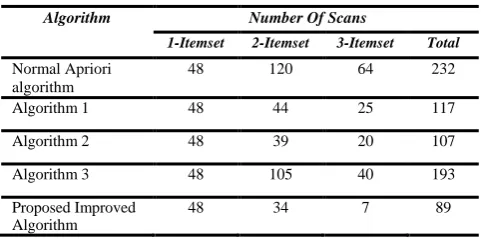
In all the above algorithms, the result is same that is {ABD}. In Table XIII and Table XIV we compare the number of scans required for each of the above discussed algorithms and find that in the proposed algorithm the number of scans is minimum. And also for the number of candidate keys generated, the proposed algorithm find out the minimum number of candidate keys.

Candidate keys generated in 1-itemset in proposed and all the other above algorithms = 6 (A, B, C, D, E, F),

Candidate keys generated in 2-itemset in proposed and all the other above algorithms= 15 (AB, AC, AD, AE, AF, BC, BD, BE, BF, CD, CE, CF, DE, DF, EF).

Candidate keys generated in 3-itemsets in proposed algorithm = 3 (ABD, ABE, BEF).

Candidate keys generated in 3-itemset in the other above discussed algorithms = 8 (ABD, ABE, ABF, ADE, AEF, BDE, BDF, BEF).

The comparisons between the number of scans and candidate keys generated are shown in Table XIII and Table XIV.

Table XIII. Comparison among the Number of Scans

Algorithm Number Of Scans

1-Itemset 2-Itemset 3-Itemset Total

Normal Apriori algorithm

48 120 64 232

Algorithm 1 48 44 25 117

Algorithm 2 48 39 20 107

Algorithm 3 48 105 40 193

Proposed Improved Algorithm

[image:5.595.301.545.73.159.2]

48 34 7 89

Table XIV. Comparison among the Number of Candidate Keys Generated

Algorithm Number Of Candidate Keys

Normal Apriori algorithm, Algorithm 1, 2 and 3

6 15 8 29

6 15 3 24

In order to establish the improvement of the proposed improvement of Apriori algorithm, the algorithms considered in this study are compared with the help of one more database. The comparison is made on the basis of the number of scans required in each of the algorithms and the number of candidate keys generated in the proposed algorithm as compared to the original Apriori algorithm.

A. Algorithm for reducing the number of scan (Algorithm 1)

[image:5.595.30.271.624.743.2]

Table XV. Original Database (Min_Support=3)

Table XVI. Frequent 1-Itemset

Sr. No. Items Support Transaction_IDs

1 I1 5 T1,T3,T7,T9,T10

2 I2 7 T2,T3,T4,T5,T6,T7,T8

3 I3 9 T1,T2,T3,T4,T5,T6,T7,T8.T10

4 I4 3 T5,T7,T8

5 I5 1 T5 (X)

6 I6 2 T7,T8 (X)

7 I7 2 T1,T2 (X)

Table XVII. Frequent 2-Itemset Sr.

No.

Transaction Items

1 T1 I1,I3,I7

2 T2 I2,I3,I7

3 T3 I1,I2,I3

4 T4 I2,I3

5 T5 I2,I3,I4,I5

6 T6 I2,I3

7 T7 I1,I2,I3,I4,I6

8 T8 I2,I3,I4,I6

9 T9 I1

10 T10 I1,I3

Sr. No.

Items Support Item with

Min_support

Transaction_IDs

1 I1I2 2 (X) I1 T1,T3,T7,T9,T10

2 I1I3 4 I1 T1,T3,T7,T9,T10

3 I1I4 1 (X) I4 T5,T7,T8

4 I2I3 7 I2 T2,T3,T4,T5,T6,T7,T8

5 I2I4 3 I4 T5,T7,T8

(6)

Table XVIII: Frequent 3-Itemset

Sr. No.

Min_support

Transaction_IDs

1 I1I2I3 2 (X) I1 T1,T3,T7,T9,T10

2 I1I3I4 1 (X) I4 T5,T7,T8

3 I2I3I4 3 I4 T5,T7,T8

B. Algorithm for reducing database size and number of scans (Algorithm 2)

Table XIX. Reduced DatabaseFor Frequent 2-Itemset

1 T1 I1,I3,I7

2 T2 I2,I3,I7

3 T3 I1,I2,I3

4 T4 I2,I3

5 T5 I2,I3,I4,I5

6 T6 I2,I3

7 T7 I1,I2,I3,I4,I6

8 T8 I2,I3,I4,I6

9 T9 I1

10 T10 I1,I3

Table XX. Frequent 2-Itemset

Sr. No.

Min_support

Transaction_IDs

1 I1I2 2 (X) I1 T1,T3,T7, T10

2 I1I3 4 I1 T1,T3,T7, T10

3 I1I4 1 (X) I4 T5,T7,T8

4 I2I3 7 I2 T2,T3,T4,T5,T6,T7,T8

5 I2I4 3 I4 T5,T7,T8

6 I3I4 3 I4 T5,T7,T8

Table XXI.Frequent 3-Itemset

Sr. No.

Min_support

Transaction_IDs

1 I1I2I3 2 (X) I1 T1,T3,T7

2 I1I3I4 1 (X) I4 T5,T7,T8

3 I2I3I4 3 I4 T5,T7,T8

C. Transaction Reduction and Matrix Method (Algorithm 3)

Figure 4. Frequent 1-Itemset.

D. Proposed Improved Algorithm

Table XXII. Frequent 2-Itemset

Sr. No. Items Support Item with

Min_support

Transaction_IDs

1 I1I2 2 (X) I1 T1,T3,T7, T10

2 I1I3 4 I1 T1,T3,T7, T10

3 I1I4 1 (X) I4 T5,T7,T8

4 I2I3 7 I2 T2,T3,T4,T5,T6,T7,T8

5 I2I4 3 I4 T5,T7,T8

6 I3I4 3 I4 T5,T7,T8

Table XXIII. Frequent 3-Itemset

Sr. No. Items Support Item with

Min_support

Transaction_IDs

1 I2I3I4 3 I4 T5,T7,T8

Now all the algorithms for the second example are compare in Table XXIV and Table XXV.

Table XXIV. Comparison among the Number of Scans

Algorithm Number Of Scans

Normal Apriori algorithm

70 60 30 160

Algorithm 1 70 26 11 107

Algorithm 2 70 24 9 103

Algorithm 3 70 54 12 136

(7)

[image:7.595.30.271.76.160.2]

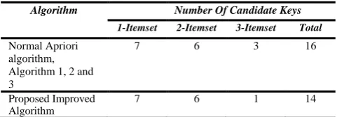
Table XXV. Comparison among the Number of Candidate Keys Generated

Algorithm Number Of Candidate Keys

Normal Apriori algorithm, Algorithm 1, 2 and 3

7 6 3 16

7 6 1 14

In this example also, the final result for all the algorithms is again the same, that is {I2, I3, I4}. And from the table it is seen that the number of scans and candidate keys generated is minimum in the proposed improved algorithm.

VI. CONCLUSION

Association rule mining is an important technique in data mining in order to discover the frequently occurring patterns in the database. Apriori algorithm is one of the oldest and efficient algorithms in the field of association rule mining. In spite of its simplicity, the Apriori algorithm suffers from a number of drawbacks. The objective of this paper is to study the limitations of Apriori algorithm and enhance the performance of the Apriori algorithm. Here an improvement of Apriori algorithm is proposed for discovering association rules in large databases. The proposed algorithm can efficiently extract the association rules between the data items in large databases. After comparing all the algorithms with the proposed improved algorithm, it can be concluded that the improved algorithm has successfully reduced the number of database scans required and the number of candidate keys generated. As less number of candidate keys is generated,

memory required to hold this candidate keys also gets reduced. But in this proposed improved algorithm, the step, where before the generation of (k+1) frequent itemsets, the transaction which contains less than (k+1) items are deleted, consumes time, as every time we have to check the database to perform this step.

VII. REFERENCES

[1] J. Han, M. Kamber, J. Pei “Data Mining Concepts and Techniques,” Morgan Kaufmann Publisher, Third Edition, Year 2012.

[2] S. Nasreen, M. A. Azamb, K. Shehzada, U. N. M. Ali Ghazanfara, “Frequent Pattern Mining Algorithms for Finding Associated Frequent Patterns for Data Streams: A Survey” Procedia Computer Science 37, pages 109 – 116, Year 2014.

[3] R. Agrawal and R. Srikant. “Fast algorithms for mining association rules,” In Proc. 1994 Int. Conf. Very Large Data Bases, pages 487–499, Santiago, Chile, September 1994.

[4] M. Al-Maolegi1, B. Arkok, AN IMPROVED APRIORI ALGORITHM FOR ASSOCIATION RULES,” International Journal on Natural Language Computing (IJNLC), vol. 3, No.1, February 2014.

[5] S. Aggarwal and R. Sindhu, An approach to improve the efficiency of apriori algorithm. PeerJ PrePrints 3:e1410 https://doi.org/10.7287/peerj.preprints.1159v1, 2015 [6] V. Mangla, C. Sarda, S. Madra, “Improving the efficiency