Page 1 of 96
Special Report
In-depth mining of clinical data: the construction of clinical
prediction model with R
Zhi-Rui Zhou1#, Wei-Wei Wang2#, Yan Li3#, Kai-Rui Jin4, Xuan-Yi Wang4, Zi-Wei Wang5, Yi-Shan Chen6, Shao-Jia Wang7, Jing Hu6, Hui-Na Zhang6, Po Huang6, Guo-Zhen Zhao6, Xing-Xing Chen4, Bo Li6, Tian-Song Zhang8
1Department of Radiotherapy, Huashan Hospital, Shanghai Medical College, Fudan University, Shanghai 200040, China; 2Department of Thoracic Surgery, The Third Affiliated Hospital of Kunming Medical University & Yunnan Provincial Tumor Hospital, Kunming 650118, China; 3Department of Anesthesiology, The Fourth Affiliated Hospital, Harbin Medical University, Harbin 150001, China; 4Department of Radiation Oncology, Shanghai Cancer Center, Shanghai Medical College, Fudan University, Shanghai 200040, China; 5Department of Urology, Changhai Hospital, The Second Military Medical University, Shanghai 200040, China; 6Beijing Hospital of Traditional Chinese Medicine, Capital Medical University, Beijing Institute of Traditional Chinese Medicine, Beijing 100010, China; 7Department of Gynecologic Oncology, The Third Affiliated Hospital of Kunming Medical University & Yunnan Provincial Tumor Hospital, Kunming 650118, China; 8Internal Medicine of Traditional Chinese Medicine Department, Jing’an District Central Hospital, Fudan University, Shanghai 200040, China
Contributions: (I) Conception and design: ZR Zhou, B Li, TS Zhang; (II) Administrative support: B Li; (III) Provision of study materials or patients: ZR Zhou; (IV) Collection and assembly of data: All authors; (V) Data analysis and interpretation: All authors; (VI) Manuscript writing: All authors; (VII) Final approval of manuscript: All authors.
#These authors contributed equally to this work.
Correspondence to: Zhi-Rui Zhou. Department of Radiotherapy, Huashan Hospital, Shanghai Medical College, Fudan University, Shanghai 200040, China. Email: [email protected]; Bo Li. Beijing Hospital of Traditional Chinese Medicine, Capital Medical University, Beijing Institute of Traditional Chinese Medicine, Beijing 100010, China. Email: [email protected]; Tian-Song Zhang. Internal Medicine of Traditional Chinese Medicine Department, Jing’an District Central Hospital, Fudan University, Shanghai 200040, China. Email: [email protected].
Introduction to Clinical Prediction Models
Background
For a doctor, if there is a certain “specific function” to predict whether a patient will have some unknown outcome, then many medical practice modes or clinical decisions will change. Such demand is so strong that almost every day we will hear such a sigh “If I could know in advance, I would certainly not do this!”. For example, if we can predict that a patient with malignant tumor is resistant to a certain chemotherapy drug, then we will not choose to give the patient the drug; if we can predict that a patient may have major bleeding during surgery, then we will be careful and prepare sufficient blood products for the patient during the operation; if we can predict that a patient with hyperlipidemia will not benefit from some lipid-lowering drug, then we can avoid many meaningless medical interventions.
As a quantitative tool for assessing risk and benefit, the clinical prediction model can provide more objective and accurate information for the decision-making of doctors, patients and health administrators, so its application is becoming more and more common. Under this kind of rigid demand, researches of clinical prediction model are in the ascendant.
The current medical practice model has evolved from empirical medicine to evidence-based medicine and then to precise medicine. The value of data has never been more important. The rapid development of data acquisition, data storage and analysis and technology of prediction in the big data era has made the vision of personalized medical treatment become more and more possible (1,2). From the perspective of the evolvement of medical practice models, accurately predicting the likelihood of a certain clinical outcome is also an inherent requirement of the current precise medical model.
This paper will summarize the researches of clinical prediction model from the concept, current application status, construction methods and processes, classification
of clinical prediction models, necessary conditions for conducting such researches and the current problems.
Concept of clinical prediction model
Clinical predictive model refers to using a parametric/semi-parametric/non-parametric mathematical model to estimate the probability that a subject currently has a certain disease or the likelihood of a certain outcome in the future (3). It can be seen that the clinical prediction model predicts the unknown by the knowing, and the model is a mathematical formula, that is, the known features are used to calculate the probability of the occurrence of an unknown outcome through this model (4,5). Clinical prediction models are generally modeled by various regression analysis methods, and the statistical nature of regression analysis is to find the “quantitative causality.” To be simple, regression analysis is a quantitative characterization of how much X affects Y. Commonly used methods include multiple linear regression model, logistic regression model and Cox regression model. The evaluation and verification of the effectiveness of prediction models are the key to statistical analysis, data modeling, and project design, and it is also the most demanding part of data analysis technology (6).
Based on the clinical issues we have studied, clinical prediction models include diagnostic models, prognostic models and disease occurrence models (3). From a statistical point of view, prediction models can be constructed as long as the outcome of a clinical problem (Y) can be quantized by the feature (X). The diagnostic model is common in cross-sectional studies, focusing on the clinical symptoms and characteristics of study subjects, and the probability of diagnosing a certain disease. The prognostic model focuses on the probability of outcomes such as recurrence, death, disability, and complications in a certain period of time of a particular disease. This model is common in cohort studies. There is another type of prediction model that predicts whether a particular disease will occur in the future based on the general characteristics of the subject, which is also
advanced variable selection methods in linear model, such as Ridge regression and LASSO regression. Keywords: Clinical prediction models; R; statistical computing
Submitted Jun 05, 2019. Accepted for publication Aug 02, 2019. doi: 10.21037/atm.2019.08.63
common in cohort studies. There are many similarities among the diagnostic model, the prognostic model and the disease occurrence model. Their outcomes are often dichotomous data and their effect indicators are the absolute risks of the outcome occurrence, that is, the probability of occurrence, not the effect indicators of relative risk such as relative risk (RR), odds ratio (OR) or hazard ratio (HR). At the technical level of the model, researchers will face with the selection of predictors, the establishment of modeling strategies, and the evaluation and verification of model performance in all of these models.
Applications of clinical prediction models
As described in the background part, clinical prediction models are widely used in medical research and practice. With the help of clinical prediction models, clinical researchers can select appropriate study subjects more accurately, patients can make choices more beneficial for themselves, doctors can make better clinical decisions, and health management departments can monitor and manage the quality of medical services better and allocate medical resources more rationally. The effects of clinical prediction models are almost reflected in any of the three-grade prevention system of diseases:
Primary prevention of disease
The clinical prediction model can provide patients and doctors with a quantitative risk value (probability) of diagnosing a particular disease in the future based on current health status, offering a more intuitive and powerful scientific tool for health education and behavioral intervention. For example, the Framingham Cardiovascular Risk Score based on the Framingham’s studies on heart clarified that lowering blood lipids and blood pressure could prevent myocardial infarction (7).
Secondary prevention of disease
Diagnostic models often use non-invasive, low-cost and easy-to-acquire indicators to construct diagnostic means with high sensitivity and specificity and to practice the idea of “early detection, early diagnosis, early treatment”, which has important significance of health economics.
Tertiary prevention of disease
The prognostic model provides quantitative estimates for probabilities of disease recurrence, death, disability and complications, guiding symptomatic treatment and
rehabilitation programs, preventing disease recurrence, reducing mortality and disability, and promoting functional recovery and quality of life.
There are several mature prediction models in clinical practice. For example, Framingham, QRISK, PROCAM, and ASSIGN scores are all well-known prediction models. The TNM staging system for malignant tumors is the most representative prediction model. The biggest advantage of TNM is that it is simple and fast, and the greatest problem is that the prediction is not accurate enough, which is far from the expectations of clinicians. The need to use predictive tools in clinical practice is far more than predicting disease occurrence or predicting the prognosis of patients. If we can predict the patient’s disease status in advance, for example, for patients with liver cancer, if we can predict whether there is microvascular infiltration in advance, it may help surgeons to choose between standard resection and extended resection, which are completely different. Preoperative neoadjuvant radiotherapy and chemotherapy is the standard treatment for T1-4N+ middle and low rectal cancer. However, it is found during clinical practice that the status of lymph nodes estimated according to the imaging examinations before surgery is not accurate enough, and the proportion of false positive or false negative is high. Is it possible to predict the patient’s lymph node status accurately based on known characteristics before radiotherapy and chemotherapy? These clinical problems might be solved by constructing a suitable prediction model.
Research approach of clinical prediction models
Clinical prediction models are not as simple as fitting a statistical model. From the establishment, verification, evaluation and application of the model, there is a complete research process of the clinical prediction model. Many scholars have discussed the research approaches of clinical prediction models (8-11). Heart Magazine recently published a review, in which the authors used risk score for cardiovascular diseases (CVD) as an example to explore how to construct a predictive model of disease with the help of visual graphics and proposed six important steps (12):
(I) Select a data set of predictors as potential CVD influencing factors to be included in the risk score; (II) Choose a suitable statistical model to analyze the
relationship between the predictors and CVD; (III) Select the variables from the existing predictors
(IV) Construct the risk score model; (V) Evaluate the risk score model;
(VI) Explain the applications of the risk score in clinical practice.
The author combined literature reports and personal research experience and summarized the research steps as shown in Figure 1.
Clinical problem determine research type selection
Clinical prediction models can answer questions about etiology, diagnosis, patients’ response to treatment and prognosis of diseases. Different research types of design are required for different problems. For instance, in regard to etiology studies, a cohort study can be used to predict whether a disease occurs based on potential causes. Questions about diagnostic accuracy are suitable for cross-sectional study design as the predictive factors and outcomes occur at the same time or in a short period of time. To predict patients’ response to treatment, cohort study or randomized controlled trial (RCT) can be applied. For prognostic problems, cohort study is suitable as there are longitudinal time logics for predictors and outcomes. Cohort study assessing the etiology requires rational selection of study subjects and control of confounding factors. In studies of diagnostic models, a “gold standard” or reference standard is required to independently diagnose the disease, and the reference standard diagnosis should be performed with blind method. That is to say, reference standard diagnosis cannot rely on information of predictors in prediction models to avoid diagnostic review bias. Assessing patients’ response to treatment is one type of interventional researches. It is also necessary to rationally select study subjects and control the interference of non-test factors. In studies of prognostic model, there is a vertical relationship between predictors and outcomes, and researchers usually expect to obtain outcome of the disease in the natural status, so prospective cohort study is the most common prognostic model and the best type of research design.
Establishment of study design and implementation protocol, data collection and quality control
Good study design and implementation protocol are needed. First, we need to review the literatures to determine the number of prediction models to be constructed:
(I) At present, there is no prediction model for a specific clinical problem. To construct a new model, generally a training set is required to construct the
model and a validation set to verify the prediction ability of the model.
(II) There are prediction models at present. To construct a new model, a validation set is applied to build the new model and the same training data set is applied to verify the prediction ability of the existing model and the new model respectively. (III) To update the existing models, the same validation
set is used to verify the prediction ability of the two models.
With regard to the generation of training data sets and validation data sets, data can be collected prospectively or retrospectively, and the data sets collected prospectively are of higher quality. For the modeling population, the sample size is expected to be as large as possible. For prospective clinical studies, the preparation of relevant documents includes the research protocol, the researcher’s operation manual, the case report form, and the ethical approval document. Quality control and management of data collection should also be performed. If data is collected retrospectively, the data quality should also be evaluated, the outliers should be identified, and the missing values should be properly processed, such as filling or deleting. Finally, the training data set for modeling and the validation set for verification are determined according to the actual situations. Sometimes we can only model and verify in the same data set due to realistic reasons, which is allowed, but the external applicability of the model will be affected to some extent.
Establishment and evaluation of clinical prediction models
Before establishing a prediction model, it is necessary to clarify the predictors reported in the previous literature, determine the principles and methods for selecting predictors, and choose the type of mathematical model applied. Usually a parametric or semi-parametric model will be used, such as logistic regression model or Cox regression model. Sometimes algorithms of machine learning are used to build models and most of these models are non-parametric. Because there are no parameters like regression coefficients, the clinical interpretation of such nonparametric models is difficult. Then fit the model and estimate the parameters of the model. It is necessary to determine the presentation form of the prediction model in advance. Currently, there are four forms commonly used in prediction models:
the prediction model tool.
(II) Nomogram. The regression coefficients of the regression model are transformed into scores through appropriate mathematical transformations
and plotted as a nomogram as a predictive model tool.
(III) Web calculator. The nature is also to convert the regression coefficients of the regression model into Figure 1 The flow chart of construction and evaluation of clinical prediction models.
Clinical Prediction Model Construction and Evaluation
Variable Screen Mehod
Prediction Model Evaluation
Regularization method
Cluster analysis
Principal component and factor analysis
No existing model Prediction Model
Construction
Parameterized model
Semi-parametric model
Nonparametric model
General linear model
Generalized linear model
Linear regression
Logisticregression
Possion regreesion
Cox proportional hazard model
Competing risk model
Machine learning method
KNN method
SVM method
Classification regression tree
Random forest method
Neural network Ridge regression
Lasso regression
Elastic network
Hierarchical clustering
K-means clustering
PAM method
Discriminant analysis
Deep learning
Already have 2 models
Already have 1 model
Have 2 datasets
Training set modeling
Validation set validation
Linear regresion
Logistic regression
Cox proportional hazard model
Lasso regression
Machine learning algorithm
Convert coefficients into scores
Draw nomogram
Draw nomogram
Screening variables, then use linear, logistic or cox method to draw nomogram
Construct non-parametric model
Discrimination
Calibration
DCA anslysis
Area Under ROC
C-Statistics
C-Index
Calibration Plot
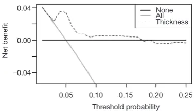
DCA Curve
Validate in one dataset
Discrimination
Calibration
DCA analysis
Area Under ROC
C-Statistics
C-Index
Calibration Plot
DCA Curve
Add/remove variables or introduce new variables
Evaluate the improvement of the new model over the old model
C-Statistics
Net Reclassification Index NRI
Integrated Discrimination Improvement IDI
scores by appropriate mathematical operations, and to make it into a website for online use.
(IV) Scoring system. The regression coefficients of the regression model are transformed into a quantifiable scoring system through appropriate mathematical operations.
The first form is mainly for linear regression model, which is a deterministic regression. The latter forms are based on parametric or semi-parametric models, the statistical nature of which is the visual representation of the model parameters. The researchers can make choices based on actual conditions. After the model is built, how to evaluate the pros and cons of the model? The evaluation and verification of the model are of higher statistical analysis technology. For example, the discrimination, calibration, clinical effectiveness and other indicators of the prediction models are evaluated to determine the performance of the models.
Validation of clinical prediction models
The effect of the prediction model is prone to change as the scenario and the population change. Therefore, a complete study of prediction model should include validation of the model. The content of the validation includes the internal validity and external validity of the model. Internal validity reflects the reproducibility of the model, which can be validated through cross-validation and Bootstrap with the data of the study itself. External validity reflects the generalizability of the model and needs to be validated with data sets not from the study itself, which are temporally and geographically independent, or completely independent.
Internal and external validation of the model are necessary steps to assess the stability and applicability of the model. The data sets for internal validation and external validation should be heterogeneous, but not to a certain extent. Generally, data from the original institution are used as training set to build the model and a part of the internal data are randomly selected to perform internal validation. Data from other institutions are selected as the external verification data set. Of course, it is best to do external data set validation. I will introduce several methods to verify internal validity.
(I) Split-half method. Randomly divide the existing data into two parts, one for building the model and the other for validating the model. The data is divided into two parts by the semi-division method for “internal verification”. Since only half of the data is used to build the model, the model is
relatively unstable. Studies with small sample sizes are not suitable for this method.
(II) Cross-validation method. This method is a further evolution of the split-half method. The half-fold cross-validation and the ten-fold cross-validation are commonly used. The half-fold cross-validation method is to divide the original data into two parts, one for establishing and the other for validating the model. Then exchange the rolls of the two parts and mutually verifying each other. The ten-fold cross-validation method is to divide the data into ten parts, and to uses nine parts for establishing the model, and the other part for verifying the model. By establishing and verifying the model ten times in this way, a relatively stable can be constructed. (III) Bootstrap method. The conventional Bootstrap
internal validity analysis method is to randomly sample a certain number of returnable cases in the original data set to build a model, and then use the original data set to verify the model. By doing random sampling, establishment and validation for 500–1,000 times, 500–1,000 models can be obtained, and the parameter distributions of the model can be summarized. Therefore, the final parameter values of the model can be determined. Bootstrap method is a fast-developing method in recent years. This method develops in the background of computer numeration increase. It is proved that models acquired through this method have higher stability than through the previous two methods. It can be speculated that Bootstrap method will be increasingly applied internal validity analysis of the prediction models. Of course, if conditions are met, we should do external validation of prediction models as much as possible to improve the external applicability of the models.
Assessment of clinical effectiveness of clinical prediction models
specificity of the model. For predicting survival outcomes, we generally evaluate whether patients can be classified into good or poor prognosis according to the prediction model. For instance, the score of each subject is calculated by Nomogram, and the patients are classified into good prognosis group and poor prognosis group according to a certain cutoff value, then a Kaplan-Meier survival curve is drawn. Decision Curve Analysis is also a commonly used method for predicting clinical effectiveness of models. From the perspective of the final purpose of the prediction model construction and study design, the best clinical effectiveness assessment is to design randomized controlled trials, and usually cluster randomized controlled trials are used to assess whether the application of prediction models can improve patient outcomes and reduce medical costs.
Update of clinical prediction models
Even with well-validated clinical prediction models, the model performance is degraded over time due to changes of disease risk factors, unmeasured risk factors, treatment measures, and treatment background, which is named the calibration drift. Therefore, clinical prediction models need to evolve and update dynamically. For example, the frequent update of the most commonly used malignant tumor TNM staging system is also because of these reasons.
Current researches of clinical prediction model can be roughly divided into three categories from the perspective of clinicians
(I) Prediction models are constructed with traditional clinical features, pathological features, physical examination results, laboratory test results, etc. The predictive variables in this type of models are more convenient for clinical acquisition and are the construction of these models is more feasible.
(II) With the maturity of radiomics research methods, more and more researchers are aware that certain manifestations or parameters of imaging represent a specific biological characteristic. Using the massive imaging parameters of color Doppler ultrasound, CT, MR or PET combined with clinical features to construct prediction models can often further improve the accuracy of the prediction models. The modeling of this type of method is based on screening the features of radiomics. The pre-workload of this type is much larger than the first method, and close cooperation between clinical department and imaging
department is needed.
(III) With wide use of high-throughput biotechnology such as genomics and proteomics, clinical researchers are attempting to explore featured biomarkers for constructing prediction models from these vast amounts of biological information. Such prediction models are a good entry point for the transformation of basic medicine into clinical medicine, but such researches require strong financial support as various omics tests of the clinical specimens need to be done. However, the input and output of scientific research are directly proportional. As the saying goes, “Reluctant children can’t entrap wolves.” Although there is nobody willing to entrap the wolf with a child, the reason is the same. Once the researches willing to put money in omics analysis are well transformed into clinic, generally the researches can yield articles with high impact factors. In addition, biological samples must be obtained, otherwise there is foundation to launch such researches.
The necessary conditions to conduct clinical prediction model from the perspective of clinicians
(I) Build a follow-up database of a single disease and collect patient information as completely as possible, including but not limited to the following: demographic characteristics, past history, family history, personal history; disease-related information such as important physical and laboratory findings before treatment, disease severity, clinical stage, pathological stage, histological grade; treatment information: such as surgical methods, radiotherapy and chemotherapy regimens, dose and intensity; patients’ outcomes: for cancer patients, consistent follow-ups are required to obtain their outcomes, which is an extremely difficult and complex task. Other information: If there is, such as genetic information. Database construction is a core competency.
of RCT and ignored the great value of real-world data. RCT data have the highest quality without doubt, but the data have been screened strictly, therefore the extrapolation of the evidence is limited. Real-world data come from our daily clinical practice, which reflects the efficacy of clinical interventions more comprehensively, and the evidence has better external applicability. However, the biggest problems of real-world study are that the data quality varies wildly and there are too many confounding factors that is difficult to identify. Therefore, it is necessary to use more complicated statistical methods to find the truth from the complicated confounding factors. It is not easy to sift sand for gold, and solid statistical foundation is like a sifter for gold. Here we need to understand that confounding factors exist objectively, because the occurrence of any clinical outcome is not the result from a single factor. There are two levels of correction for confounding factors. One is correction at the experimental design stage, which is the top-level correction, such as equalizing confounding factors between groups by randomization and enough sample size. This is also the reason why RCT is popular: as long as the sample size is enough and randomization is correct, the problem of confounding factors is solved once and for all. The second is after-effect correction through statistical methods, which is obviously not as thorough as the RCT correction, but the second situation is closer to the real situation of our clinical practice.
(III) Sample size. Because there are many confounding factors in real-world research, a certain sample size is necessary to achieve sufficient statistical efficacy to discern the influence of confounding factors on the outcome. A simple and feasible principle for screening variables by multivariate analysis is that if one variable is included in multivariate analysis, there should be 20 samples of the endpoint, which is called “1:20 principle” (13,14).
(IV) Clinical research insight. Construction of clinical prediction model is to solve clinical problems. The ability to discover valuable clinical problems is an insight that is cultivated through widely reading and clinical practice.
Issues currently faced in the development of prediction model
(I) Low clinical conversion rate. The main reason is that
the clinical application of the prediction model needs to be balanced between the accuracy and the simplicity of the model. Imagine if there is a model that is as easy to use as TNM staging, but more accurate than TNM staging, what choices would you make?
(II) Most of the clinical prediction models were constructed and validated based on retrospective datasets and validation is rarely performed in the prospective data. Therefore, the stability of the results predicted by the models was comparatively poor. (III) Validation of most clinical prediction models is based
on internal data. Most articles have only one dataset. Even if there are two datasets, one to construct and the other to validate, but the two datasets often come from the same research center. If the validation of the prediction model can be further extended to dataset of another research center, the application value of the model will be greatly expanded. This work is extremely difficult and requires multi-center cooperation. Moreover, most of the domestic centers do not have a complete database for validation, which comes back to the topic “database importance” discussed earlier.
Brief summary
The original intention of the clinical prediction model is to predict the status and prognosis of diseases with a small number of easily collected, low-cost predictors. Therefore, most prediction models are short and refined. This is logical and rational in an era when information technology is underdeveloped and data collection, storage and analysis are costly. However, with the development of economy and the advancement of technology, costs of data collection and storage have been greatly reduced and technology of data analysis is improving. Therefore, clinical prediction model should also break through the inherent concept, with application of larger amounts of data (big data) and more complex models as well as algorithms (machine learning and artificial intelligence) to serve doctors, patients, and medical decision makers with more accurate results.
In addition, from the perspective of a clinical doctor conducting clinical researches, the following four principles should be grasped when conducting researches of clinical prediction models:
construction is the core competitiveness, while prediction model is only a technical method; (III) We need to raise awareness that RCT is as
important as real-world study. Both are ways to provide reliable clinical evidence;
(IV) Validation of the models requires internal and external cooperation, so we should strengthen the internal cooperation of scientific research and improve the awareness of multi-center scientific research cooperation.
Variable screening method in multivariate regression analysis
Background
Linear regression, Logistic regression and Cox proportional hazards regression model are very widely used multivariate regression analysis methods. We have introduced details about the principle of computing, application of associated software and result interpreting of these three in our book Intelligent Statistics (15). However, we talked little about independent variable screening methods, which have induced confusion during data analysis process and article writing for practitioners. This episode will focus more on this part.
Practitioners will turn to statisticians when they are confronted with problems during independent variable screening, statisticians will suggest the application of automatic screening in software, such as Logistic regression and Cox regression in IBM SPSS, which have suggested seven methods for variable screening as follow (16,17):
(I) Conditional parameter estimation likelihood ratio test (Forward: Condition);
(II) Likelihood Ratio Test of Maximum Partial Likelihood Estimation (Forward LR);
(III) Wald chi-square test (Forward: Wald);
(IV) Conditional parameter estimation likelihood ratio test (Backward: Condition);
(V) Likelihood Ratio Test of Maximum Partial Likelihood Estimation (Backward: LR);
(VI) Wald chi-square test (Backward: Wald);
(VII) Enter method (all variable included, default method).
Actually, in clinical trial report, many authors will adopt one of these screening methods. I am going to talk about: they will perform univariate regression analysis of every variable one by one firstly; those with P value less than 0.1
will be included in the regression formula (here P value could be less than 0.05 or 0.2, but in common condition, P value can range between 0.05–0.2). This method is very controversial. For practitioners, how to choose a better method is really an optional test. To be honest, there is no standard answer. But we still have some rules for better variable screening:
(I) When the sample size is larger enough, statistical test power is enough, you can choose one from those six screening methods we mentioned before. Hereby we introduce a method which can help you evaluate the test efficiency quickly: 20 samples (events) are available for each variable. For example, in Cox regression test, if we include 10 variables associated with prognosis, at least 200 patients should be recruited to evaluate endpoint events, such as death (200 dead patients should be included instead of 200 patients in total). Because those samples without endpoint event won’t be considered to be test effective samples (13,14). (II) When the sample size is not qualified for the first
condition or statistical power is not enough for some other reasons, widely used screening method in most clinical report should be applied. You can perform univariate regression analysis of every variable one by one firstly; those with P value less than 0.2 will be included in the regression formula. As we mentioned before, this method is quite controversial during its wide application.
(III) Even the second screening method will be challenged during practice. Sometimes we find some variables significantly associated with prognosis may be excluded for its disqualification in already set-up screening methods. For example, in a prostate cancer prognosis study, the author find Gleason score is not significantly associated with prognosis in the screening model, while Gleason score is a confirmed factor for prostate cancer prognosis in previous study. What should we do now? In our opinion, we should include those variables significantly associated with prognosis in our analysis though they may be disqualified in statistical screening method for professional perspective and clinical reasons.
Disputes and consensus
The discussion about variable screening has been going on for a long time. Statistician consider it with very professional perspective, however clinical doctors will not always stick to these suggestions. It is very hard to distinguish the right and the wrong for actual problem during clinical study, such as small simple size; limited knowledge to confirm the exact factors for the outcome. However, we still have some standards for reference during screening. During the review about good quality clinical studies published on top magazines, 5 conditions will be considered during variable screening (18):
(I) Clinical perspective. This is the most basic consideration for variable screening. Medical statistical analysis can be meaningless if it is just statistical analysis. Based on professional view, confirmed factors significantly associated with outcome, such as Gleason score in prostate cancer, should be included in regression model. We do not need to consider its statistical disqualification in variable screening.
(II) S c r e e n i n g b a s e d o n u n i v a r i a t e a n a l y s i s . Independent variable included in multivariate analysis based on the results of the univariate analysis. Variables with significant P value should be included in multivariate regression. If P<0.1, we think it is “significant”. Sometimes P<0.2 or P<0.05 will be considered “significant”. P value can range according to sample size. Big sample size will be with small P value. Small sample size will be with relatively big P value. This screening method is quite common in already published articles, even in top magazines. Though this method has been questioned by statisticians, it is still being used for no method because no more precise and scientific option available now. Even statisticians could not find better replacement. Before we find better option to replace this one, it is better to have one than to have none.
(III) The variables would be chosen based on the influence of the confounding factor “Z” on the test factor or the exposure factor “X”. To be specific, we will observe if “X” will affect dependent variable “Y” when “Z” change or not. First run the basic model that only includes “X”, record the regression coefficient β1, and then add “Z” to the model to see how much the β1 changes. It is generally
considered that the β1 change exceeds 10%, and the variable needs to be adjusted, otherwise it is not needed. This method is different from the second one because of quantification of confounding factor effect. This is not perfect because the effect “Z” and “X” exert on “Y” could be affected by other confounding factors. This thought may lead to logical confusion. Complicated methodological problem will be left for further exploration by the smart ones. In our opinion, this is acceptable option for variable screening, especially for those programs with very specific targets. We can confirm the effect of “X” on independent “Y”. This effect is real and what we do can regulate these confounding factors. (IV) Choosing right number of variables that will
eventually be included in the model. is very important. This is a realistic problem. If the sample size is large enough and the statistical performance is sufficient, we can use the variable screening method provided by the statistical software to automatically filter the variables, and we can filter out the variables that are suitable for independent impact results in statistical. “Ideal is full, the reality is very skinny”. Sometimes we will consider a lot of variables, while the sample size is pretty small. We have to make compromise between statistical efficiency and variable screening. Compromise can bear better results (13,14).
(V) Above we listed four commonly used variable screening methods. Many other variable screening methods, such as some methods based on model parameters: determination coefficient R2, AIC,
likelihood logarithm, C-Statistics, etc. can be an option also. The fact that too many variable screening methods is a good evidence to support a view that there is no best available during practice. This article aims to help us find the right screening method instead of confirming the best one or worst one. Choosing the fittest one according to actual condition is the goal of this article.
The methods for recruiting different types of variables
Continuous variable
dichotomous variable or ordinal categorical variable, then put them into the regression formula. We have already changed former continuous variable into categorical variable by this way. We do this transformation because the variable may be not linear to the outcome. Some other relationship instead of linear one may present.
Continuous variable transformation summary
When continuous variable is included in regression model, the original variable, as far as possible, should be included in this model and actual needs should be considered also. The variable can be transformed based on some rules. Two-category grouping, aliquot grouping, equidistant grouping, and clinical cut-off value grouping are present for better professional explanation. By optimal truncation point analysis, we convert continuous variables into categorical variables and introduce them into the regression model as dummy variables. In regression model, the continuous variable can be present in different ways. We will give specific examples as follow. No matter which way it will present, the general principle is that this change is better for professional interpretation and understanding (19-21).
Normal transformation
For continuous variables which are in normal distribution, this is not a problem. However, when we confronted with data which is not fit normal distribution, we can make transformation based on some function, then these data will be normalized. And it will fit the regression model. Original data can be normalized by different function, such as Square Root method, LnX method, Log10X method
and (1/X) etc., according to its own character. If you have normalized the original data, you should interpret the variable after normal transformation instead of the original ones in the regression model or you can reckon the effect of the original independent variable exerting on the original dependent variable according to the function used in the transformation.
For example, the authors have done normality test in the article they published in JACC, 2016 (21). The original expression is as follows: Normality of continuous variables was assessed by the Kolmogorov-Smirnov test. The method of normality test includes using the parameters of the data distribution (the skewness value and the kurtosis value) and using the data distribution graph (histogram, P-P diagram, Q-Q diagram). Or some nonparametric test methods (Shapiro-Wilk test, Kolmogorov-Smirnov test) will be applied to help us to
evaluate the normality of data. In their research, variables such as troponin I, NT-proBNP, or corin is fit abnormal distribution. So, the author describes baseline characters of these recruited objects by median (quartile - third quartile). For example, the median of Troponin I is 4.5 (1.8–12.6) ng/mL. Then multivariable linear regression is performed to analyze corin. The original expression is as follows: multiple linear regression analysis was applied to determine factors influencing corin levels. Levels of troponin I, NT-proBNP, and corin were normalized by Log10 transformation. Variables like troponin I, NT-proBNP, corin have been normalized by function Log10.
After that, they have been included into multivariable linear regression. Then, the author performed Cox regression. Though there is no specific requirement for Cox regression, Log10 function was used to normalize troponin I,
NT-proBNP and corin. All these three variables have been included in multivariable linear regression model for consistency with original ones.
Transformation for each change of fixed increment
If continuous variable is introduced directly into the model in its original form, the regression parameter is interpreted as the effect of the change in the dependent variable caused by each unit change. However, sometimes the effect of this change may be weak. Therefore, we can transform the continuous independent variables into a categorical variable by fixed interval, in an equidistant grouping, and then introduce them into the model for analysis. This grouping is good for better understanding and application for patients. For example, we include patients whose age range between 31 to 80 years old. We can divide it into groups of 10–40, 41–50, 51–60, 61–70, 71–80 according to10 years age interval. Then five already set dummy variables will be included into the model for analysis. However, if the variable range a lot, grouping according to the methods we mentioned before will lead to too many groups and too many dummy variables, which will be quite redundant during analysis. It will be very hard for clinical interpretation too. In the opposite, some data with a small range and cannot be grouping again, it cannot be transformed into categorical variable also. Then, what should we do when we are confronted with these two situations?
interval + unit”. We will illustrate 2 examples in this article. The mean of oxygen uptake efficiency slope is 1,655 U and 5–95% population will change from 846 to 2,800 U. It is really a big range. If the original data is put into formula, per 1 U change will lead to very week change of HR, which is meaningless in clinical practice. If it is transformed into categorical variables, many groups will appear. So, the author includes per 100 U change into the model and finds that the mortality risk will decrease 9% (HR =0.91, 95% CI: 0.89–0.93) when oxygen uptake efficiency slope increases in per 100 U. Another example is variable Peak RER. The median is 1.08 U and 5–95% population will change from 0.91–1.27 U. It is really a small range. If the original data is put into formula, per 1 U change will lead to very big change of HR. In clinical practice, patients with a change of 1 U are quite rare and this outcome will be of limited practicality. It will be very hard for categorical variable transformation too for its small range. So, the author includes per 0.1U change into the model and finds that the mortality risk will decrease 6% (HR =0.94, 95% CI: 0.86–1.04) when Peak RER increases per 0.1 U. However, it is not statistically significant.
Then, how can we do this transformation? If we want to change the factor from each1 unit to 100 units, it will be 100 times larger. We only need to divide the original variable by 100 and then to include into the model. Similarly, if we want to change the factor from 1 unit to 0.1 unit, the change is reduced by 10 times. It is only necessary to multiply the original variable by 10 and include it into the regression model.
Transformation of each standard deviation
In clinical study, we get another transformation method: independent variable change at per SD increase. Let us see an article published in JACC in 2016 (20). Age and systolic pressure are included in the model as per SD increase. The age increase at per SD, the risk of atherosclerotic heart disease (ASCVD) increases by 70% (HR =1.70, 95% CI: 1.32–2.19). Systolic blood pressure (SBP) increased at per SD, the risk of ASCVD increases by 25% (HR =1.25, 95% CI: 1.05–1.49). Here the author has put continuous variable into the model with the form of per SD increase. Assuming that the variables are fit to normal distribution, the area within the mean ±1 SD interval is 68.27%, while the mean value is ±1.96, the area within the SD interval is 95%. If the mean value is ±2.58, the area within the SD interval is 99%. We can tell that if the data range within 4 SD, about 95% samples will be covered. Therefore, new variables, especially for those rare ones which are still unclear in clinical
interpretation, we can put per SD into the model. This can guide the patient to see that he or she is within the range of several standard deviations of the population distribution level according to his or her actual measurement results, and then to assess how much the corresponding risk will change.
It is very simple to do this kind of transformation. We can do it by these two ways:
(I) Before constructing the regression model, the original continuous variables should be normalized, and the normalized independent variables are brought into the regression model. The regression coefficient obtained is the influence of the dependent variable on each dependent SD. (Attention: Only independent variables are normalized here).
(II) If the original variables are not normalized, the original variables can be directly brought into the model, and the Unstandardized Coefficients are obtained, and then the standard deviation of the independent variables is calculated by multiplying the standard deviation of the independent variables, which is also called Standardized Coefficients. This is the effect of the dependent variable for each additional SD of the independent variable.
Rank variable
Non-ordered & multi-categorical variable
Non-ordered & multi-categorical variable is very common variable style. Usually, there are several possible values in a multi-categorical variable, while there is no hierarchical relationship between each other. For example, race (1= white, 2= black, 3= yellow, 4= others), method of drug administration (1= oral, 2= hypodermic, 3= intravenous, 4= others), they are all non-ordered category variables. When non-ordered multi-category variable are in Logistic or Cox regression model, we need to set dummy variable before we brought them in the model. We will introduce the dummy variable setting methods in the follow.
Dummy variable setting methods
(I) Indicator: this method is used to specify the reference level of the categorical variable. The parameter calculated here is referred to the last or first level of the variable. It is depending on whether you choose the first or last in the following Reference Category. (II) Simple: this method can calculate the ratio of each
level of the categorical variable compared to the reference level.
(III) Difference: this method can compare the categorical variable with the mean of all levels. It is totally the opposite of Helmert. So, it is also called Reversed Helmert. For example, mean of level 2 can be compared with the mean of level 1; the mean of level 3 can be compared with that of level 1 and level 2 respectively and so forth. If the coefficient becomes small at a certain level and is not statistically significant, the effect of the categorical variable on the risk ratio is reached its plateau. This option is generally used for ordered-categorical variables, such as smoking doses. Assuming that the researchers analyze them as independent non-ordered multi- category variable, it will be meaningless.
(IV) Helmert: we will compare the level of categorical variable with the mean of the following levels. If the coefficient of a certain level increases and is statistically significant, it indicates that the categorical variable has an impact on the risk rate from this level. It can also be used in ordered-categorical variables. (V) Repeated: the levels of the categorical variables are
compared with the levels adjacent to them, except for the first level, where the “previous level” is used as the reference level.
Brief summary
We have already summarized the screening methods and variables transformation methods. The absolutely perfect way is not valid in really world. But we can still choose the right way. Comparing with choose one method in haste, we need more scientific solutions. There is one way for reference: you can construct multiple models (mode1, model 2, model 3…) based on previous published clinical trials, especially those with high impact score and get the objective outcome of each model. It actually is sensitivity analysis. Different models will be constructed based on different variables. Some variables, which may be closely related to the true world, will lead to relatively stable outcome even in different models. This is also a way to reach the goal. We will not judge it here. We want to find out the most stable factor for the outcome from results.
During the construction of predictive model, we will have specific consideration except for variables screening in all these possible variables. For example, TNM staging for malignant tumors are widely used for its easily application in clinical practice instead of its prediction value of in prognosis. Actually, TNM staging prediction value is just so-so. Here we have to talk about another question: How can we assess the accuracy and simplicity of the model? More variable may lead to more accurate prediction of a model while it will be much more difficult for clinical application. Sometimes a comprise should be made.
Method of building nomogram based on Logistic regression model with R
Background
the proportion of false positive or false negative is high. Is it possible to predict the patient’s lymph node status accurately based on known characteristics before radiotherapy and chemotherapy? If we can build such a prediction model, then we can make clinical decisions more accurately and avoid improper decision-making caused by misjudgment. More and more people are becoming aware of the importance of this problem. At present, researchers have made vast efforts to build prediction models or improve existing prediction tools. The construction of Nomogram is one of the most popular research directions.
When do you choose Logistic regression to build a prediction model? This is related to the clinical problems and the clinical outcomes set up. If the outcomes are dichotomous data, unordered categorical data or ranked data, we can choose Logistic regression to construct the model. Generally unordered Logistic regression and ranked Logistic regression are applied in unordered multi-categorical or ranked data outcomes, but the results are difficult to explain. Thus, we generally convert unordered multi-classification or ranked data outcomes into dichotomous outcomes and use dichotomous Logistic regression to construct the model. Outcomes such as “whether liver cancer has microvascular infiltration” and “recurrence of lymph node metastasis before rectal cancer” mentioned above belong to dichotomous outcomes. Dichotomous Logistic regression can be used for constructing, evaluating and validating the prediction model (15).
The screening principles for model predictors are consistent with the principles described in section 2. In addition, we need to consider two points: on the one hand, the sample size and the number of independent variables included in the model should be weighed; on the other hand, we should also weigh the accuracy of the model and the convenience to use the model, to finally determine the number of independent variables entering the prediction
model (13,14,17).
In this section, we will use two specific cases to introduce the complete process of constructing a Logistic regression prediction model with R language and drawing a Nomogram. For complex statistical principles, we choose to avoid as much as possible, and we would focus on the R implementation process of this method.
We can summarize the process of constructing and verifying clinical prediction models into the following eight steps (22):
(I) Identify clinical issues and determine scientific hypotheses;
(II) Determine research strategies of prediction models according to previous literatures;
(III) Determine the predictors of the predictive model; (IV) Determine the outcome variables of the prediction
model;
(V) Construct the prediction model and calculate model predictors;
(VI) Assessment of model discrimination ability; (VII) Assessment of model calibration;
(VIII) Assessment of clinical effectiveness of the model. Research process of prediction models construction can be referred to Figure 2.
[Case 1] analysis
[Case 1]
Hosmer and Lemeshow studied the influencing factors of low birth weight infants in 1989. The outcome variable is whether to give birth to low birth weight infants (Variable name: “low”; Dichotomous variable; 1= low birth weight, which is infant birth weight <2,500 g; 0= not low birth weight). The possible influencing factors (independent variables) include: maternal pre-pregnancy weight (lwt, unit: pound); maternal age (age, unit: year); whether the Figure 2 Research process and technical routes of three prediction models.
Identify clinical
issues Determine research strategies Determine the predictors Determine the outcome
Construct the prediction model
Assessment of model discrimination
ability
Assessment of model calibration
Assessment of clinical effectiveness Identify clinical
issues
Construct the prediction model
Determine research strategies
Assessment of model discrimination
ability
Determine the predictors
Assessment of model calibration
Determine the outcome
mother smokes during pregnancy (smoke, 0= no, 1= yes); number of preterm births before pregnancy (ptl, unit: time); high blood pressure (ht, 0= no, 1= yes); uterus stress to the contraction caused by stimulation, oxytocin, etc. (ui, 0= no, 1= yes); visits to community doctors in the first three months of pregnancy (ftv, unit: time); race (race, 1= white, 2= black, 3= other).
[Case 1] interpretation
In this case, the dependent variable is dichotomous (whether or not a low birth weight infant is delivered). The purpose of the study is to investigate the independent influencing factors of low birth weight infants, which is consistent with the application conditions of binary Logistic regression. As there is only one data set in this case, we can use this data set as the training set to model, and then use Bootstrap resampling method to perform internal model validation in the same data set. It should be noted here that we can also randomly divide the data set into a training set and an internal validation set according to a 7:3 ratio, but we did not do so considering the sample size. We will demonstrate the prediction model construction of low birth weight infants and the rendering of Nomogram with R language below. The data were collected and named “Lweight.sav”, which is saved in the current working path of R language. The data and code can be downloaded from the attachments in this Section for readers to practice. The specific analysis and calculation steps are as follows:
(I) Screen the independent influencing factors affecting low birth weight infants and construct a Logistic regression model;
(II) Visualize the Logistic regression model and draw a Nomogram;
(III) Calculate the discrimination degree (C-Statistics) of the Logistic model;
(IV) Perform internal validation with resampling method and draw the Calibration curve.
[Case 1] R codes and results interpretation
Load the “foreign” package for importing external data in .sav format (IBM SPSS style data format). Load the rms package to build the Logistic regression model and to plot the nomogram (23):
library(foreign) library(rms)
Import the external data in .sav format and name it “mydata”. Then set the data to the structure of data frame, and display the first 6 lines of the data frame.
mydata<-read.spss(“Lowweight.sav”) mydata<-as.data.frame(mydata) head(mydata)
## id low age lwt race smoke ptl ht ui ftv bwt ## 1 85 normal weight 19 182 black no smoking 0 no pih yes 0 2523 ## 2 86 normal weight 33 155 other no smoking 0 no pih no 3 2551 ## 3 87 normal weight 20 105 white smoking 0 no pih no 1 2557 ## 4 88 normal weight 21 108 white smoking 0 no pih yes 2 2594 ## 5 89 normal weight 18 107 white smoking 0 no pih yes 0 2600 ## 6 91 normal weight 21 124 other no smoking 0 no pih no 0 2622
Data preprocessing: set the outcome variable as a dichotomous variable, define “low birth weight” as “1”, and set the unordered categorical variable “race” as a dummy variable.
mydata$low <- ifelse(mydata$low ==“low weight”,1,0) mydata$race1 <- ifelse(mydata$race ==“white”,1,0) mydata$race2 <- ifelse(mydata$race ==“black”,1,0) mydata$race3 <- ifelse(mydata$race ==“other”,1,0)
Load the data frame “mydata” into the current working environment and “package” the data using function datadist().
attach(mydata) dd<-datadist(mydata) options(datadist=‘dd’)
Fit the Logistic regression model using function lrm() and present the results of the model fitting and model parameters. Note: The parameter C of Rank Discrim Indexes. in the model can be directly read. This is the C-statistics of model “fit1”. According to the calculation results, the C-Statistics is 0.738 in this example. The meaning and calculation method of C-Statistic will be further explained in the following sections.
fit1<-lrm(low ~age+ftv+ht+lwt+ptl+smoke+ui+race1+race2, data = mydata, x = T, y = T)
fit1
## Logistic Regression Model ##
## lrm(formula = low ~ age + ftv + ht + lwt + ptl + smoke + ui + ## race1 + race2, data = mydata, x = T, y = T)
##
## Model Likelihood Discrimination Rank Discrim. ## Ratio Test Indexes Indexes ## Obs 189 LR chi2 31.12 R2 0.213 C 0.738 ## 0 130 d.f. 9 g 1.122 Dxy 0.476 ## 1 59 Pr(> chi2) 0.0003 gr 3.070 gamma 0.477 ## max |deriv| 7e-05 gp 0.207 tau-a 0.206 ## Brier 0.181
##
## ht=pih 1.7631 0.6894 2.56 0.0105 ## lwt -0.0137 0.0068 -2.02 0.0431 ## ptl 0.5517 0.3446 1.60 0.1094 ## smoke=smoking 0.9275 0.3986 2.33 0.0200 ## ui=yes 0.6488 0.4676 1.39 0.1653 ## race1 -0.9082 0.4367 -2.08 0.0375 ## race2 0.3293 0.5339 0.62 0.5374 ##
Use function nomogram() to construct the Nomogram object “nom1” and print the Nomogram. The result is shown in Figure 3.
nom1 <-nomogram(fit1, fun = plogis,fun.at =c(.001, .01, .05, seq(.1,.9, by = .1), .95, .99, .999),
lp = F, funlabel =“Low weight rate”) plot(nom1)
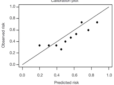
Use the function calibrate() to construct the calibration curve object “cal1” and print the calibration curve. The result is shown in Figure 4.
cal1 <-calibrate(fit1, method =‘boot’, B =100) plot(cal1,xlim =c(0,1.0),ylim =c(0,1.0)) ##
## n=189 Mean absolute error=0.037 Mean squared error=0.00173 ## 0.9 Quantile of absolute error=0.054
From the calculation results of Logistic regression model fit1 above andFigure 3, it is obvious that the contribution
of some predictors to the model are negligible, such as the variable “ftv”. There are also some predictors that may not be suitable for entering the prediction model as dummy variable, such as “race”, and the clinical operation is cumbersome. We can consider conversing the un-ordered categorical variables into dichotomous variables properly and involve them into the regression model. The adjusted codes are as follows:
First of all, according to the actual situation, we convert the unordered categorical variable “race” into a binominal variable. The standard of conversion is mainly based on professional knowledge. We classify “white” as one category and “black and other” as another.
mydata$race <-as.factor(ifelse(mydata$race==“white”, “white”, “black and other”))
Use function datadist() to “package the current data set.
dd<-datadist(mydata) options(datadist =‘dd’)
Figure 4 Calibration curve based on model “fit1”.
Figure 3 Nomogram based on model “fit1”.
1.0
0.8
0.6
0.4
0.2
0.0
0.0 0.2 0.4 0.6 0.8 1.0
B=100 repetitions, boot Predicted Pr{low=1}Mean absolute error=0.035 n=189 Apparent
Bias-corrected ldeal
Actual pr
obability
Points
age
ftv
ht
lwt
ptl
smoke
ui
race1
race2
Total points
Low weight rate
0 10 20 30 40 50 60 70 80 90 100
no pih
smoking
no smoking
no
1
1
pih 45 40 35 30 25 20 15 10
260 240 220 200 180 160 140 120 100 80
0 20 40 60 80 100 120 140 160 180 200 220 240 260 280
0.05 0.1 0.2 0.3 0.4 0.5 0.6 0.7 0.8 0 4
0 2
6
3
yes
0
0 1
Exclude the variable “ftv that contributes less to the result from the regression model, then reconstruct model “fit2” and display the model parameters. It can be seen that C-Statistics =0.732.
fit2<-lrm(low ~ht+lwt+ptl+smoke+race, data=mydata, x = T, y = T) fit2
## Logistic Regression Model ##
## lrm(formula = low ~ ht + lwt + ptl + smoke + race, data = mydata, ## x = T, y = T)
##
## Model Likelihood Discrimination Rank Discrim. ## Ratio Test Indexes Indexes ## Obs 189 LR chi2 28.19 R2 0.195 C 0.732 ## 0 130 d.f. 5 g 1.037 Dxy 0.465 ## 1 59 Pr(> chi2) <0.0001 gr 2.820 gamma 0.467 ## max |deriv| 1e-05 gp 0.194 tau-a 0.201 ## Brier 0.184
##
## Coef S.E. Wald Z Pr(>|Z|) ## Intercept 0.7743 0.8303 0.93 0.3511 ## ht=pih 1.6754 0.6863 2.44 0.0146 ## lwt -0.0137 0.0064 -2.14 0.0322 ## ptl 0.6006 0.3342 1.80 0.0723 ## smoke=smoking 0.9919 0.3869 2.56 0.0104 ## race=white -1.0487 0.3842 -2.73 0.0063 ##
Use the function nomogram() to construct Nomogram object “nom2”, and print the Nomogram. The result is
shown in Figure 5.
nom2 <-nomogram(fit2, fun = plogis,fun.at =c(.001, .01, .05, seq(.1,.9, by=.1), .95, .99, .999),
lp = F, funlabel =“Low weight rate”) plot(nom2)
Nomogram interpretation: It is assumed that a pregnant woman has the following characteristics: pregnancy-induced hypertension, weight of 100 pounds, two premature births, smoking, and black. Then we can calculate the score of each feature of the pregnant woman according to the value of each variable: pregnancy-induced hypertension (68 points) + weight 100 pounds (88 points) + two premature births (48 points) + smoking (40 points) + black (42 points) =286 points. The probability of occurrence of low birth weight infants with a total score of 286 is greater than 80% (22,24). Note that the portion exceeding 80% in this example is not displayed on the Nomogram. Readers can try to adjust the parameter settings to display all the prediction probabilities with the range of 0–1.
Use function calibrate() to construct the calibration curve object “cal2” and print the calibration curve. The result is shown in Figure 6 below.
cal2 <-calibrate(fit2, method =‘boot’, B =100) plot(cal2,xlim =c(0,1.0),ylim =c(0,1.0)) ##
## n=189 Mean absolute error=0.021 Mean squared error=0.00077 ## 0.9 Quantile of absolute error=0.036
Figure 5 Nomogram based on model “fit2”.
Points
ht
lwt
ptl
smoke
race
Total points
Low weight rate
0 10 20 30 40 50 60 70 80 90 100
pih
no pih
smoking
black and other
white no smoking
260 240 220 200 180 160 140 120 100 80
0 20 40 60 80 100 120 140 160 180 200 220 240
0.05 0.1 0.2 0.3 0.4 0.5 0.6 0.7 0.8 2
3 1
Interpretation of calibration curve: In fact, the calibration curve is a scatter plot of the probability of actual occurrence versus prediction. Actually, the calibration curve visualizes the results of Hosmer-Lemeshow fit goodness test, so in addition to the calibration curve, we should also check the results of Hosmer-Lemeshow fit goodness test. The closer to Y = X the prediction rate and the actual occurrence rate are, with p value of Hosmer-Lemeshow goodness-of-fit test greater than 0.05, the better the model is calibrated (24). In this case, the Calibration curve almost coincides with the Y = X line, indicating that the model is well calibrated.
[Case 2] analysis
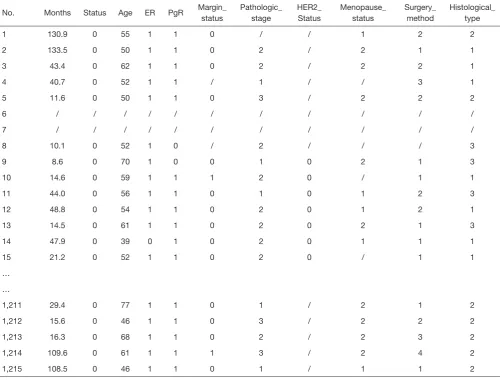
[Case 2]
Survival in patients with advanced lung cancer from the North Central Cancer Treatment Group. Performance scores rate how well the patient can perform usual daily activities. Total 10 variates:
(I) inst: Institution code; (II) time: Survival time in days;
(III) status: censoring status 1=censored, 2=dead; (IV) age: Age in years;
(V) sex: Male=1 Female=2;
(VI) ph.ecog: ECOG performance score (0=good 5=dead);
(VII) ph.karno: Karnofsky performance score (bad=0-good=100) rated by physician;
(VIII) pat.karno: Karnofsky performance score as rated by patient;
(IX) meal.cal: Calories consumed at meals; (X) wt.loss: Weight loss in last six months.
The case data set is actually survival data. In order to be consistent with the theme of this Section, we only consider the binominal attribute of the outcome (status 1 = censored, 2 = dead). Again, we select the Logistic regression model to construct and visualize the model, draw Nomogram, calculate C-Statistics, and plot the calibration curve.
[Case 2] R codes and its interpretation
Load survival package, rms package and other auxiliary packages.
library(survival) library(rms)
Demonstrate with the “lung” data set in the survival package. We can enumerate all the data sets in the survival package by using the following command.
data(package = “survival”)
Read the “lung” data set and display the first 6 lines.
data(lung) head(lung)
## inst time status age sex ph.ecog ph.karno pat.karno meal.cal wt.loss ## 1 3 306 2 74 1 1 90 100 1175 NA
## 2 3 455 2 68 1 0 90 90 1225 15 ## 3 3 1010 1 56 1 0 90 90 NA 15 ## 4 5 210 2 57 1 1 90 60 1150 11 ## 5 1 883 2 60 1 0 100 90 NA 0 ## 6 12 1022 1 74 1 1 50 80 513 0
You can use the following command to display the variable descriptions in the lung dataset.
help(lung)
Variable tags can be added to dataset variables for subsequent explanation.
lung$sex <-factor(lung$sex, levels =c(1,2),
labels =c(“male”, “female”))
According to the requirements of rms package to build the regression model and to draw Nomogram, we need to “package“ the data in advance, which is the key step to draw Nomogram, Use the command “?datadist” to view its detailed help documentation.
dd=datadist(lung) options(datadist=“dd”)
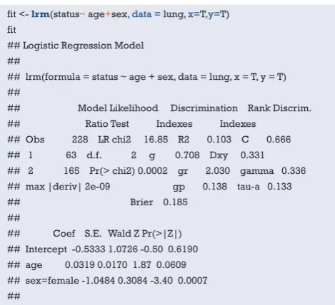
Using “status” as the dependent variable, “age” and “sex” as the independent variables, the Logisitc regression model “fit” was constructed, and the model parameters were shown. It can be seen that C-Statistics =0.666.
Figure 6 Calibration curve based on model “fit2”.
1.0
0.8
0.6
0.4
0.2
0.0
0.0 0.2 0.4 0.6 0.8 1.0
B=100 repetitions, boot Predicted Pr{low=1}Mean absolute error=0.022 n=189 Apparent
Bias-corrected ldeal
Actual pr