ABSTRACT
LIN, SHANGMIN. A Data-Driven Method for Probabilistic Damping Assessment in Power Systems Using Synchrophasors. (Under the direction of Aranya Chakrabortty.)
© Copyright 2014 by ShangMin Lin
A Data-Driven Method for Probabilistic Damping Assessment in Power Systems Using Synchrophasors
by ShangMin Lin
A thesis submitted to the Graduate Faculty of North Carolina State University
in partial fulfillment of the requirements for the Degree of
Master of Science
Electrical Engineering
Raleigh, North Carolina
2014
APPROVED BY:
Ning Lu Subhashish Bhattacharya
BIOGRAPHY
ACKNOWLEDGEMENTS
TALBE OF CONTENTS
LIST OF TABLES . . . vi
LIST OF FIGURES . . . vii
Chapter 1 Introduction . . . 1
Chapter 2 Recapitulation of Bayesian Inference . . . 4
2.1 Bayes’ Rule . . . 4
2.2 Metropolis-Hasting MCMC Method . . . 5
Chapter 3 Data based Clustering in Power Systems . . . 8
3.1 Multidimensional Scaling . . . 8
3.2 Correlograms . . . 9
3.3 Other clustering Method . . . 12
Chapter 4 Bayesian Modeling of Faults . . . 13
4.1 Bandpass filter and FFT design . . . 14
4.2 Description of Our Bayesian Model . . . 17
4.3 Prior Probability Distributions . . . 18
4.4 Likelihood Function Derivation . . . 18
4.5 Posterior Computation . . . 21
4.6 Combine with MDS plot . . . 21
Chapter 5 Case Studies . . . 23
5.1 Case Study 1: Two-Area Kundur System . . . 23
5.1.1 Two Area Model and Noise . . . 23
5.1.2 Simulation Result . . . 25
5.1.3 Metropolis-Hasting Demonstration . . . 25
5.2 Case Study 2: 50-bus Australian Power System . . . 26
5.2.1 Randomness of Laplacian Matrix . . . 28
5.2.2 Randomness of the Damping matrix . . . 29
5.2.3 Stochastic Changing . . . 30
5.2.4 Prior distribution . . . 30
5.2.5 MDS plot for Clustering . . . 33
5.2.6 Bayesian Modeling Result . . . 34
Chapter 6 Test Results with Real PMU data . . . 40
6.1 Prior Distribution from Historical Data . . . 40
6.2 MDS for clustering . . . 41
6.3 Posterior Damping Calculation . . . 41
References. . . 46
Appendix . . . 50
LIST OF TABLES
LIST OF FIGURES
Figure 3.1 PMU Time Series . . . 10
Figure 3.2 Correlograms Example . . . 11
Figure 4.1 Whole Algorithm Diagram . . . 14
Figure 4.2 FFT Example . . . 15
Figure 4.3 FIR compared with IIR . . . 16
Figure 4.4 Bodeplot for Different Windows . . . 16
Figure 5.1 Kundur Power System Model . . . 23
Figure 5.2 Frequency Compared Plot for Randomness . . . 24
Figure 5.3 Posterior Distributions . . . 26
Figure 5.4 MCMC Samples . . . 27
Figure 5.5 Histogram of Metropolis-Hasting Samples . . . 27
Figure 5.6 50 Buses Power System Model . . . 28
Figure 5.7 Example of Frequency Data with Randomness . . . 31
Figure 5.8 Fitting Plot for Prior Distribution . . . 32
Figure 5.9 Output Voltage Angle Plot for Australian Power System Model . . . 34
Figure 5.10 Time Series Plot for Australian Power System Model . . . 35
Figure 5.11 MDS for Australian Power System Model . . . 35
Figure 5.12 Correlograms for Australian Power System Model . . . 36
Figure 5.13 Output Frequency Comparison Plot . . . 37
Figure 5.14 FFT Plot . . . 38
Figure 5.15 Posterior Distribution of fAustralian Power System Model . . . 38
Figure 5.16 Posterior Distribution of fAustralian Power System Model . . . 39
Figure 6.1 MDS Plot for Real PMU Data . . . 42
Figure 6.2 Four Substations Frequency Plot for Real PMU Data . . . 43
Chapter 1
Introduction
Following the Northeast blackout of 2003, Wide-Area Measurement System (WAMS) technology using Phasor Measurement Units (PMUs) has largely matured for the North American grid [1]. Different from traditional data acquisition systems, PMU provides preciser and higher frequency sampling which enables real-time synchronized monitoring of large power systems itself as well as its electro-mechanical oscillation. Over the past decade, under the direction of the North American Synchrophasor Initiative (NASPI), WAMS researchers have developed a multitude of signal processing algorithms by which electro-mechanical modes of oscillation, and their corresponding damping factors and residues can be computed efficiently from Synchrophasor data [2], [3], [4], [5] and [6]. Well know method like Eigensystem Realization Algorithm (ERA) and majority of other algorithms which has been developed are based on small-signal linear models of the grid, and ignore the impacts of the significant nonlinearities inherent in actual power grid models.
ERA [8] or Prony [9]. With this issue of inaccurate damping estimation from PMU data using traditional deterministic methods, and the increasing number of PMUs in the grid, operators are struggling to understand how gigantic volumes of real-time PMU data can be efficiently processed and utilized to generate accurate predictions of damping, especially for the inter-area modes, so that appropriate control actions can be taken following a disturbance like small region contingency.
Motivated by this problem, in this paper we present a data-driven probabilistic approach to characterize and identify disturbance events from the perspective of small-signal stability. The two main metrics of our interest are the frequency and damping of inter-area oscillation modes. We treat damping as a stochastic uncertainty arising from the unrealistic assumptions made about the nonlinearities of the grid model, and then use a Bayesian modeling approach to predict which substations may have the large probability of showing compared low damping factors for the inter-area oscillation modes extracted from real-time PMU data. Finally, we use a Multi-dimensional Scaling (MDS) approach to identify clustering patterns of coherent substations in power system parallel from these PMU data so that the operators can perform appropriate control action manually based on the damping predictions for only a subset of substation in entire power system. It thus saves us tremendous time and work for analysis in large power system.
Among large amount of probabilistic data approach, Bayesian modeling is growing of usage rapidly these decays. It offers a number of advantages such as ability to obtain data-driven statistical measures, make predictions, compare models, and handle uncertainty. Moreover, it is a method to update the probability estimate for a hypothesis as additional evidence is acquired. In other words, it has the ability to making predictions based on previous knowledge of data. There is a few cases of studies in power system which applied Bayesian modeling approach or Bayesian Inference. One study is about simulation of weather parameters such as wind direction, wind speed and ambient temperature using Bayesian modeling approach to evaluate the transmission overload risk [16]. There are also studies in using Bayesian modeling approach to incorporate of engineering experience for prediction of transformer failure to quantify the expected impacts on service reliability [17].
Chapter 2
Recapitulation of Bayesian Inference
In our work we use Bayesian modeling framework to identify faults and their locations. The framework allows us to exploit the abundance of PMU data containing streaming time series data of fundamental power system quantities such as phase angles, voltages, and frequencies to model probabilities of faults occurring at different locations in a power grid.
There are a number of data mining and machine learning approaches that can be suitably applied to analyze and explore power system data. However Bayesian methods offer a number of advantages such as ability to make inferences and predictions based on observed data; incor-porate information from past events as prior probabilities; describe uncertainty in the modeling process; and provide ability to compare different competing models. Bayesian approach is com-putationally intensive though, but advancements in applications of methods such as Markov Chain Monte Carlo (MCMC) have allowed application of Bayesian methods to computational data analysis problems.
2.1
Bayes’ Rule
ac-cording to Bayes’ rule:
p(θ|D) = p(D|θ)×p(θ)
p(D) (2.1)
where
• θstands for an unknown variable whose probability may be affected by data.
• D corresponds to new data that is observed in current time were not used in computing the prior probability.
• p(θ), the prior probability, is the probability ofθbefore data D is observed. This proba-bility usually comes from historical data computing.
• p(θ|D), the posterior probability, is the probability of θ given data D, i.e., after current data is observed. This is what we want to know: the probability of a unknown variable given the observed data.
• p(D|θ) is the probability of observing dataDgiven a certain valueθ, which is the likelihood function.
• p(D), the marginal likelihood or marginal probability. This is the probability for dataD. This factor is the same for all possible valueθ being considered.
2.2
Metropolis-Hasting MCMC Method
function, then the posterior distribution function will come out with the same function form as the prior. However, in most cases likelihood function is not the prior conjugate function; the unknown parameters space like temperature can be moderately large too. Therefore, a large class of random sampling method have been developed, which can be refereed as Markov chain Monte Carlo (MCMC) methods.
Suppose there is no analytical formulas for the posterior distribution after the prior and likelihood is calculated since the reason we stated before. We need to generate representative samples from the distribution. The percentiles and other distribution variables should be close approximation to the true percentiles and other variables from the distribution. In other words, if we can get a large set of samples from posterior distribution, then we can approximate all sorts of useful characteristics of the posterior distribution.
Metropolis-Hasting is one of the MCMC method that is used in this article and thus intro-duced here. It is a statistic method for obtaining a sequence of random sample from a probability distribution when direct sample is difficult. It proceed as follows:
Generate a starting value of unknown variableθ0
fort= 1 to ndo
Randomly draw a candidate θ∗ from the jumping distributionJ(θ∗|θt−1) Calculate the probability ratio: r=min(1,QQ(θ(θt−1∗|Y|Y)×)×JJ(θ(θt−1∗|θ|tθ−1∗)))
Generate a random number U from uniform distribution U nif(0,1)
if U 5r then
θt=θ∗
else
θt=θt−1
end if
end for
If it is the case, then in the calculation of probability ratior, the Jumping distribution for both numerator and denominator sides can be cancel out since Normal Distribution is symmetrical.
Q(θ|Y) stands for the calculation of prior times likelihood function states in equation 2.1 while Y is the data we observed.
This algorithm processes by randomly attempting to generate samples based on previous sample, ie. move the sample place, sometimes accepting (U 5 r) the moves and sometimes rejecting (U > r) and thus remaining in place. The acceptance ratio r indicates how probable the new proposed samples is with respect to the current sample, according to the function
Chapter 3
Data based Clustering in Power
Systems
Besides the posterior prediction of dampingdi, a parallel application that we propose is to use the available PMU data to identifycoherent clusteringof generators. This means that, we first apply techniques by which one can identify which of the n substations (assuming that these substations are in close vicinity of generation sites) are coherent with each other, and thereafter apply the Bayesian inference described in next chapter only to one or two substations from each coherent group. Thus, the clustering plot will be build in real-time during the event as data is streaming in. If the result predicts that the ith substation has high probability of damping below a given threshold value, then all other stations belonging to the same coherent group as theith station will be alarmed, and possibly isolated, or at least prepared to be isolated if need be. This approach will save significant amount of computational time for posterior computation as now only a reduced number of PMU data streams are being used.
3.1
Multidimensional Scaling
between points in high dimensions and produces an embedding in a low-dimensional space (typically in two dimensions), such that the original inter-point distance relationships among the points are preserved. Several examples of using MDS can be seen in [19], [20], [21] and [22]. In our method, input to MDS algorithm is a matrix containing pair-wise similarity scores
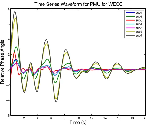
that represent metric distances between pairs of substations. Similarity scores among substa-tions are obtained by computing Euclidean distances (orL2 norm) between the substation time series vectors, though other, more complex types of metrics discussed in [23] may also be used for computing similarity scores.The time series we used in this work is the relative phase angle in PMU data. We first select a PMU site as reference and calculate relative phase angle be-tween substations and this reference site. The reason for using relative phase angle is that it can remove some part of global trend. Figure 6.1 shows a plot produced by MDS, in which points represent individual substations and spatial proximity among the points indicates similarities between corresponding substations; that is, similar substations are closer to one another in the plot. Both MATLAB and R have build-in function to calculate Euclidean distance matrix for time series and MDS plot. In our case, we use MATLAB to accomplish this work.
3.2
Correlograms
0 2 4 6 8 10 12 14 16 18 20 −6 −4 −2 0 2 4 6 8 Time (s)
Relative Phase Angle
Time Series Waveform for PMU for WECC
sub1 sub2 sub3 sub4 sub5 sub6 sub7
Figure 3.1: Time series plot from PMU data at seven substations.
sub1 sub2 sub3 sub4 sub5 sub6 sub7
sub1 1.0000000 0.8654021 0.3038602 0.9875319 0.9485746 0.7254576 0.6982585
sub2 0.8654021 1.0000000 0.3530227 0.8629839 0.8416195 0.8337659 0.7970494
sub3 0.3038602 0.3530227 1.0000000 0.2980921 0.2898170 0.3400887 0.3217194
sub4 0.9875319 0.8629839 0.2980921 1.0000000 0.9543428 0.7271880 0.7000111
sub5 0.9485746 0.8416195 0.2898170 0.9543428 1.0000000 0.7038048 0.6778258
sub6 0.7254576 0.8337659 0.3400887 0.7271880 0.7038048 1.0000000 0.9548087
sub7 0.6982585 0.7970494 0.3217194 0.7000111 0.6778258 0.9548087 1.0000000
substn_1
substn_2
substn_3
substn_4
substn_5
substn_6
substn_7
3.3
Other clustering Method
Chapter 4
Bayesian Modeling of Faults
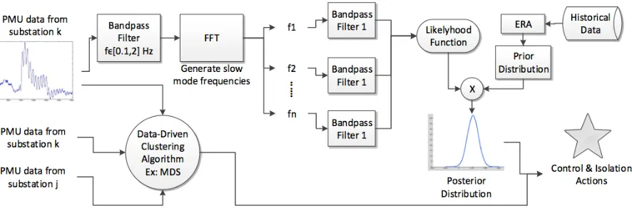
We use a Bayesian framework to model disturbances in the grid. The choice of Bayesian method follows from its simplicity as well as for its ability to handle uncertainty [28]. Physical variables such as voltage, phase angle, and frequency measured by PMUs at the substations are streamed to a control center following a disturbance, and damping factor embedded in those dynamic responses is predicted by applying a probabilistic prediction technique. The different steps of the entire algorithm are shown in Figure 4.1. The prediction is executed in an iterative fashion, i.e., the result for posterior probability distribution this event can be combined into historical data for new prior for Bayesian modeling approach of next event.
Figure 4.1: This diagram shows the whole procedure for our Bayesian probabilistic damping assessment.
4.1
Bandpass filter and FFT design
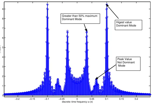
Our objective is to capture damping factors of the inter-area oscillation modes from PMU data, and both the prior and the likelihood functions is used inter-area oscillation mode for posterior estimation. To extract the most accurate contribution of the inter-area modes, we pass the PMU data-streams through three different stages of filtering. Since inter-area modes typically fall within 0.1 and 2 Hz, we first pass the data through a band-pass finite impulse response (FIR) filter with pass-band [0.1,2] Hz. Thereafter, we pass the filter output through a Fast Fourier Transform (FFT) so that we can detect exact frequencies at which the dominant modes lie. Knowledge of each dominant frequency is needed for constructing our likelihood function. The definition of dominant mode that should be detected and analyzed by Bayesian modeling approach differ from cases and usage. In our work, the highest peak as long as any peak that greater than 50% of highest one in FFT spectrum is regarded as dominant mode and will be analyzed. Figure 4.2 illustrates this concept in one FFT plot.
−0.2 −0.15 −0.1 −0.05 0 0.05 0.1 0.15 0.2 0
1 2 3 4 5 6 7 8 9
discrete−time frequency ω (π)
| X(
ω
) |
Greater than 50% maximum Dominant Mode
Higest value Dominant Mode
Peak Value Not Dominant Mode
Figure 4.2: This FFT plot illustrate what peak should be regarded as dominant mode in our detection. Besides the highest value, the second highest peak is greater than 50% of highest value thus it is dominant mode. Note that FFT plot is symmetrical thus we should only focus on one side of plot.
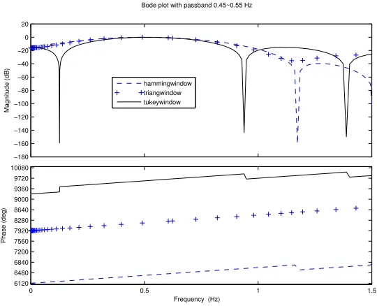
significant modal participation in the data, and hence are of no use for our analysis in any case. Normally, IIR filter has narrower band than FIR filter with identical order. However, IIR filter tend to change the damping of slow mode because it utilizes previous output term. Figure 4.3 shows how IIR filter decrease damping of a slow mode term compared to FIR filter result. FIR filter is thus chosen for the second set of bandpass filter after FFT, as showed in figure 4.1. Tukey window is selected to fulfill the notch (or narrow passband). Figure 4.4 illustrates this window gives filter narrower passband compare to Triangular window and Hamming window.
2 4 6 8 10 12 −0.15 −0.1 −0.05 0 0.05 0.1 0.15 0.2 Time(s) Value Original Signal Signal passed IIR Signal passed FIR
Figure 4.3: This plot shows a slow mode signal waveform itself and after IIR (dash line) and FIR filter. The FIR filter output follows the original signal closely while that IIR filter has lowered the damping factor.
−180 −160 −140 −120 −100 −80 −60 −40 −20 0 20 Magnitude (dB)
0 0.5 1 1.5
6120 6480 6840 7200 7560 7920 8280 8640 9000 9360 9720 10080 Phase (deg)
Bode plot with passband 0.45~0.55 Hz
Frequency (Hz) hammingwindow triangwindow tukeywindow
4.2
Description of Our Bayesian Model
We consider the measured frequency at substationi (i= 1,2, ..., n) to be expressed as
ωi(t) =fi(dij, t) + ˜ωi(t), (4.1) where fi is the true value of the frequency and ˜ωi(t) represents random perturbations around the true value. The latter can be partly filtered out by passing the data through the first set of band pass filter (BPF). The function ∆fi, is frequency data minus 60 Hz, in general, can be written as:
∆fi=
X
j=1:m
Aije−Dijtsin(λijt), dij =−cos(tan−1
λij
Dij
) (4.2)
where, dij is the damping factor of jth slow mode contained in the ith frequency measurement, and m is the total number of frequency components in the [0.1,2] Hz range, i.e., the number of slow modes. The Bayesian formulation to compute probability distributions of damping identified from PMU data at theith substation is written as [28]
p(dij|ωi(t))
| {z }
posterior
∝ p(di)
| {z }
prior
p(ωi(t)|dij)
| {z }
likelihood
. (4.3)
Note that the damping dij is simply denoted by a single subscript i for the prior probability distributions because we consider all dominant oscillation modes observed across all slow modes for historical data in substationi. On the other hand, for computing the likelihood function and the corresponding posterior probability distribution, however, we need to separate the damping of each dominant slow mode as a result of which both subscripts i and j are retained in the damping argument for this function.
is slow mode frequency ofjth slow mode contained in theith frequency measurement. We next describe the construction of the prior probability distribution function p(di) in (4.3), which is the first step of Bayesian estimation.
4.3
Prior Probability Distributions
Prior knowledge about disturbance events in a practical power system may be limited as a result of which Gamma distribution may be assumed for modeling the prior probability distribution, the choice of Gamma distribution is tested and discussed in chapter 5.2.4. As more PMU data are observed the Bayesian computation process can be repeated successively, and the updated probability distributions of the damping factors may be used as priors of subsequent iterations. The initial Gamma form can be written as:
p(di) =
βαi
i Γ(αi)
dαi−1
i e
−βidi (4.4)
The parameters of the Gamma distribution probability density function, i.e., shape (αi) and rate (βi) are determined from historic PMU data. This can be done by selecting a large set of available PMU data from the nsubstations over a set of past events, and computing αi and βi from damping factors of dominant slow modes corresponding to each substationiusing standard modal decomposition algorithms such as ERA or Prony.
4.4
Likelihood Function Derivation
Next, we derive the likelihood functionp(ωi(t)|dij) from (4.3). Considering the input disturbance to be an unit impulse, the output response of the frequencyfican be obtained by simply taking the Laplace transform offi in (4.2) as
L{fi(t)}= X j=1:m
Fij(s), X
j=1:m
Aijλij (s+Dij)2+λ2ij
If there is no measurement noise, then using bilinear transformation the discrete-time frequency-domain representation of the measured frequency signal ωi(k) at substation i with sampling time periodT can be written as:
ωi(z) = X
j=1:m
ωij(z)
= X
j=1:m
AijλijT2(z+ 1)2
4(z−1)2+ 4D
ijT(z2−1) +T(D2ij+λ2ij)(z+ 1)2
.
(4.6)
Equation (4.6) shows that ωij(k) has second-order linear homogeneous recurrence relations after k>4. This recurrence can be written as follows:
aijωij(k) =−bijωij(k−1)−cijωij(k−2) (4.7) where aij = (DijT + 2)2+ (λijT)2, bij = 2T2(Dij2 +λ2ij)−8 and cij = (DijT −2)2 + (λijT)2. Therefore, the likelihood function p(ωi(t)|dij) can be treated as a time-series, whose sample value at the kth time instant depends only on the previous two samples as (for notational simplicity we skip both subscriptsiand j for the parameters and the measurements)
p(ω(t)|d) =p(ω(1), ω(2), ω(3), ..., ω(`)|d)
=p(ω(1)|d)×p(ω(2)|d, ω(1))×p(ω(3)|d, ω(2), ω(1))×...
×p(ω(`)|d, ω(`−1), ω(`−2), ..., ω(1)) =p(ω(1)|d)p(ω(2)|d, ω(1))×
`
Y
k=3
p(ω(k)|d, ω(k−1), ω(k−2))
In the ideal case, (4.7) gives us the exact value of the measured signal ω(k), k being the sampling instant. However, in reality, the signal is bound to be corrupted by both process noise and measurement noise. The process noise is modeled as an additive load-induced disturbance term in the acceleration equation of the swing dynamics as
where xl here is the state variable in power system dynamic model, it contains phase angle and frequency data for each generator or substation, Ml is the inertia, ¯Pml is the mechanical power input, and ¯Pel is the electrical power output of thelth generator.Wl(t) denotes a Wiener process at timet, which is a stochastic process that satisfies:
1. W(0) = 0
2. The function t→W(t) is almost surely everywhere continuous 3. W(t+δt)−W(t)∼√σtN(0,1).
Here N(0,1) is zero-mean unity variance Gaussian noise. Coefficient σ is the magnitude of Gaussian noise. If we convert (4.8) to its discrete-time transfer function, equivalent to (4.6), then
σWl(t) can be integrated to the input side. Since the PMU data is a discrete-time signal with constant sampling rate, Gaussian noise for every time step can be extracted from the Weiner process function by subtracting the measured data value from the previous one. Following this concept, the likelihood function can be computed iteratively by the following pseudo code:
—input— data,D, Frequency, σ
T = 301,ω= 2π×Frequency,log likelihood= 0
a= 4 + 4×T×D+ (D×T)2+ (ω×T)2
b= 2(D×T)2+ 2(ω×T)2−8
c= 4 + (D×T)2+ (ω×T)2−4×T ×D
fork= 2 to `do
Noise=[a(data(k)-data(k−1))+ b(data(k−1)-data(k−2))+c(data(k−2)-data(k− 3))]/(ωT)
tmp = 1
σ√2πexp(− N oise2
2σ2 )
log likelihood= log likelihood+log(tmp)
end for
Prob =elog likelihood
where a, band c follow from (4.7),D follows from (4.2),` is the length of data, and ‘data’ represents the filtered slow mode response of the frequency measured at any given station (after the second set of BPF). By default, we assume data(t) =0 for allk <1.
4.5
Posterior Computation
The posterior distribution p(dij|ωi(t)) describes uncertainty about dij given the observed data
ωi(t) inith substation. The posterior is proportional to the product of the prior and likelihood distributions, as shown in (4.3). The prior Gamma distribution is relatively simpler to construct, as described before. On the other hand, our likelihood function is more complicated since it involves the product of`functions, one for each sample. Hence, direct sampling is difficult (the interested reader is referred to the topic of Conjugate Priors in [28, pages 77-95] for details). The most common way is to apply Metropolis algorithm or Gibbs sampling [28, pages 117-188] to obtain posterior samples, and fit them to construct the posterior distribution. However, this approach can be too time-consuming, especially for real-time or near-real-time applications like ours. Since we already know that for a stable system the damping factor will be in the set [0,1], for testing instability we consider the setdi∈[−1,1]. By way of this assumption, we can normalize the right-hand side of (4.3), by integration and thus obtain the posterior probability distribution of di.
4.6
Combine with MDS plot
Chapter 5
Case Studies
5.1
Case Study 1: Two-Area Kundur System
5.1.1 Two Area Model and Noise
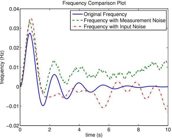
model, showed in figure 5.1 as given in [30]. A disturbance is assumed to occur at the terminal bus of Generator 1, and the frequency of Generator 3 is measured by a PMU with measurement noise. We can easily calculate the eigenvalue of power system model matrix and get damping value in this case. In this chapter we would like to exam the performance of likelihood function itself compared results from ERA so we don’t want to include the influence of prior. There-fore, the flat distribution is used for prior, which means prior probability density function is 1 everywhere. Flat prior distribution is often used when there is no previous knowledge for the unknown variable in Bayesian inference.
0 2 4 6 8 10
−0.02 −0.01 0 0.01 0.02 0.03 0.04
Frequency Comparison Plot
time (s)
frequency (Hz)
Original Frequency
Frequency with Measurement Noise Frequency with Input Noise
Figure 5.2: Plot of output frequency curves. Blue curve shows frequency of generator 3 without any noise; green curve shows frequency of generator 3 with measurement noise while red curve shows frequency of generator 3 with process input noise.
In order to exam the performance, two types of noise are added to the frequency mea-surements of Generator 3. Brownian noise ˜ω3 is directly added to the measured values, i.e.,
ω3(t) =f3(t) + ˜ω3. The magnitude of ˜ω3 is chosen to be about 6.67% of the residue of the slow
to excite the system, we insert a small random term in the input series fort >0. This random term is generated from a uniform distribution [−1,1] with its magnitude being 6.67% of the impulse value. Figure 5.2 shows the plots of the original frequency, frequency with measurement noise, and frequency with input noise.
5.1.2 Simulation Result
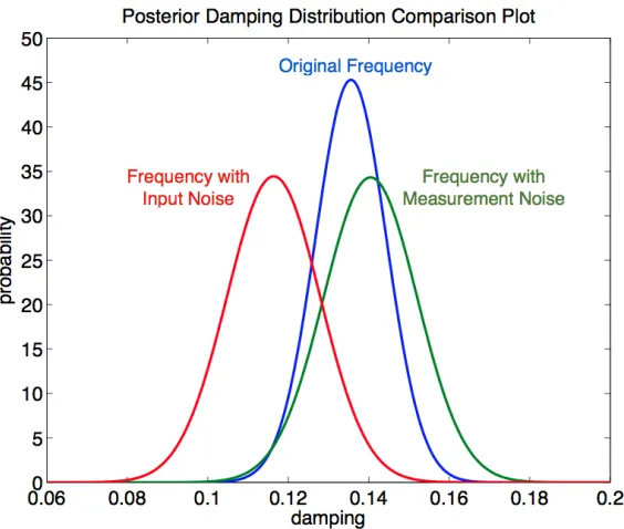
These plots are next passed through ERA to test their respective accuracies. Damping value is obtained as 0.1625 by ERA for the measurement noise case, which deviates from the real damping value 0.1362, i.e., by about 20%. ERA also generates 5 slow modes with different damping values for the input noise case, even when there is only 1 slow mode in the 2-area Kundur system. This clearly shows that if we use ERA to estimate damping in presence of model uncertainties, the estimates may be highly imprecise. On the other hand, our Bayesian modeling approach is used for these two output noise frequency data. FFT is not applied here because the slow mode frequency is known and directly applied to likelihood function, the effect of frequency difference caused likelihood function deviation is then removed as well. The posterior probability distribution plot by Bayesian inference for the original frequency measurement, as well as the two noisy cases are shown in Figure 5.3. Although the posterior probability distribution changes in the noisy conditions, the real damping value 0.1362 is still in its plausible region. By integration of these curves, we can predict the probability of dto be under a threshold value, sayd∗. Using this prediction the operator can identify the station with high possibility for unstable oscillation during contingency, and thereby use the MDS plot to execute control actions on the entire coherent group which this station belongs to.
5.1.3 Metropolis-Hasting Demonstration
Figure 5.3: Posterior probability distribution of damping in frequency of generator 3 under different cases. Peak damping value of blue distribution curve (no noise case) is 0.1362; peak damping value of green distribution curve (measurement noise case) is 0.1165; peak damping value of red distribution curve (input noise case) is 0.1405
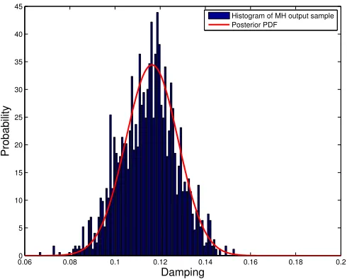
from this two area system with process noise (input noise) as an example. The result MCMC damping data is showed in figure 5.4; the normalized histogram plot with previous posterior PDF curve are plot in figure 5.5. As we can see, the integration method is reasonable and nearly identical with the results from Metropolis-Hasting Algorithm. Nevertheless, Metropolis-Hasting Algorithm is more time consuming and thus not selected in our real time damping assessment data modeling approach.
5.2
Case Study 2: 50-bus Australian Power System
0 500 1000 1500 2000 2500 0.08
0.09 0.1 0.11 0.12 0.13 0.14 0.15 0.16
Markov Chains over Damping samples
Damping
n sample number
Figure 5.4: 2000 MCMC damping samples from the 2-area Kundur power system model with input noise.
0.060 0.08 0.1 0.12 0.14 0.16 0.18 0.2
5 10 15 20 25 30 35 40 45
Damping
Probability
Histogram of MH output sample Posterior PDF
Figure 5.6: The 50 buses with 14 generators Australian model power system. It is divided into four coherent areas shown by different colors.
clustering idea combined with the Bayesian modeling approach.
A model of a prototype Australian power system, with 50 buses and 14 generators divided into 4 areas, is shown in figure 5.6. Generator 1 to 5 is belong to area 1; generator 6 and 7 is belong to area 2; generator 8 to 11 is from area 3 and generator 12, 13 and 14 is from area 4. There should be three inter-area slow mode in this system. Although the model is more complicated, it is still a linear model and there shouldn’t be any difference between each time the model is run since there is no randomness.
To model it like real PMU cases and for our purpose, we added several randomness term (different from input and output noise state in previous section) in this model state as follow:
5.2.1 Randomness of Laplacian Matrix
Mx˙ = 0 I L D
x+
0 I
∆Pm (5.1)
where state variable x is the angular position and angular velocity of generator in power system; Pm is the mechanical power input from the turbine; M is the inertia constant for generator; D is the damping matrix in power system and L is the Laplacian matrix from power system. Laplacian matrix is constructed by machines states, machine variables and line impedances between machines. Thus there should be some randomness for Laplacian matrix each time we model it through MATALB. We model randomness by multiply each row with a random number, as it shows in equation 5.2. This random numberr is sampled from uniformly distributed from 0.5 to 1.5, which means 50% of uncertainty is added to each row of Laplacian matrix. By this way of randomization, 0L0 can still remain as Laplacian matrix which is a essential characteristic in power system.
L=
L1,1 L1,2 · · · L1,n
L2,1 L2,2 · · · L2,n ..
. ... . .. ...
Ln,1 Ln,2 · · · Ln,n
; L0 =
r1 r2 .. . rn ×
L1,1 L1,2 · · · L1,n
L2,1 L2,2 · · · L2,n ..
. ... . .. ...
Ln,1 Ln,2 · · · Ln,n
(5.2)
5.2.2 Randomness of the Damping matrix
D=
D1 0 0 · · · 0
0 D2 0 · · · 0
0 0 D3 0
..
. ... . ..
0 0 0 0 Dn
; D0 =
R1 R2 .. . Rn ×
D1 0 0 · · · 0
0 D2 0 · · · 0
0 0 D3 0
..
. ... . ..
0 0 0 0 Dn
(5.3)
5.2.3 Stochastic Changing
For normal simulation using MATLAB model like previous chapter, the element value in state variables matrix remain the same during simulation. In real world, however, power system is variate every second due to the variation of load, operation of generators and changing in transmission parameter. In this chapter our modeling approach thus makes model parameters changing during the simulation, i.e. making parameters being stochastic. The randomness pa-rameters r and R in previous paragraph are perturbing by 30% of their original value during simulation, results output frequency more realistic. Output frequency under these three kind of randomness can be seen in figure 5.7.
5.2.4 Prior distribution
0 1 2 3 4 5 6 7 8 9 10 −8
−6 −4 −2 0 2 4 6x 10
−3
Time (s)
Frequency Peturbation
Event1 Event2 Event3
0 0.1 0.2 0.3 0.4 0.5 0.6 0.7 0.8 0.9 1 0
1 2 3 4 5 6
Histograms Fitting plot for Damping
Damping
Probability
Histogram Gamma Normal Beta
Figure 5.8: Histogram plot and fitting distributions waveform for Normal, Beta and Gamma distribution.
distribution as our prior should be carefully considered.
Most common and tradition way to decide prior distribution is by fitting. Trying to fit the huge size of historical data with different kinds of distribution and compare the similarity between them. We ran the Australian power system several times as historical data to decide the prior distribution.
As in figure 5.8, among three fitting distributions, Gamma distribution follows the curve of histogram closer than other two distributions. Beta distribution ramp up quickly when damping is close to zero, which does not seems to follow the data. Normal distribution on the other hand has worst fitting result as its peak is far away from real peak. There is still some points that Gamma distribution can not follow. Nevertheless, Gamma distribution is chose for our work as prior distribution. In future works, we can find more distribution for fitting test and try to find more suitable distribution for our modeling than Gamma distribution.
5.2.5 MDS plot for Clustering
One event from the model is analyzed using Bayesian modeling approach and MDS technique. According to the previous chapter, we first calculated the reference phase angle data and passed them to ERA to extract the slow modes component. Afterward, we use MATLAB build-in MDS function for MDS plot of this event. Figure 5.9 shows the raw phase angle data at generators while figure 5.10 shows the relevant slow mode component of phase angle at generators. The result MDS plot is shown in figure 5.11. Note that there is no generator 1 in MDS plot since it is used as reference generator. Clustering pattern is pretty obvious in MDS plot. We can point out generator 2 to 5 is belong to a cluster and roughly say that generator 8, 9 and 10 belongs to another cluster and the rest generators may from one or two cluster. This observation basically agree with the model setting for this 14 generators Australian power system model.
0 1 2 3 4 5 6 7 8 9 10 −3.5 −3 −2.5 −2 −1.5 −1 −0.5 0 0.5
Raw Voltage Angle Data
Time (s)
Voltage Angle Deviation (rad)
Gen1 Gen2 Gen3 Gen4 Gen5 Gen6 Gen7 Gen8 Gen9 Gen10 Gen11 Gen12 Gen13 Gen14
Figure 5.9: Plot of output voltage angles of 14 generators.
any generators where its possibility for damping below a given threshold value is too large, we need to take further control and protection actions on the whole cluster of generators.
5.2.6 Bayesian Modeling Result
We then use Bayesian Inference describe in figure 4.1 to asses the damping value in these generators at this event. The generators output frequency data can be seen in figure 5.13. First we used FFT to detect dominant slow modes frequency of the output frequency data among these generators. A plot of FFT spectrum of generator 3 can be seen in figure 5.14. We then input these peak values (1.4Hz for generator 3) as well as frequency data to likelihood function. Multiplied with the prior distribution, posterior probability density distribution plot is then generated in figure 5.15 and figure 5.16.
0 1 2 3 4 5 6 7 8 9 10 −2 −1 0 1 2 3 4 5 6 7
Reference Slow Mode Voltage Angle Data
Time (s)
Voltage Angle Deviation (rad)
Gen2 Gen3 Gen4 Gen5 Gen6 Gen7 Gen8 Gen9 Gen10 Gen11 Gen12 Gen13 Gen14
Figure 5.10: Plot of slow mode components from ERA of output reference voltage angles of 14 generators.
−10 −5 0 5 10 15
−6 −4 −2 0 2 4 6 8 gen2 gen5 gen6 gen8 gen9 gen10 gen11 gen12 gen13 gen14 gen3gen4 gen7
MDS plot of an Event at 14 Generators model
x
y
Gen2
Gen3
Gen4
Gen5
Gen6
Gen7
Gen8
Gen9
Gen10
Gen11
Gen12
Gen13
Gen14
0 1 2 3 4 5 6 7 8 9 10 −0.04
−0.03 −0.02 −0.01 0 0.01 0.02 0.03 0.04
Frequency of Generators
Time (s)
Frequency
Generator1 Generator3 Generator9 Generator11 Generator14
Figure 5.13: This plot shows the output frequency data for selected generators in power system model.
−0.4 −0.3 −0.2 −0.1 0 0.1 0.2 0.3 0.4 0
0.1 0.2 0.3 0.4 0.5 0.6
Discrete FFT spectrum
discrete−time frequency ω (π)
| X(
ω
) |
Figure 5.14: FFT spectrum of frequency data at generator 3. Peak value is at about 0.095π, which is 1.42 Hz for slow mode frequency.
−0.030 −0.02 −0.01 0 0.01 0.02 0.03 0.04 0.05 0.06 50
100 150 200 250
Posterior Probability Density Distribution
Damping
Probability
Generator1 Generator3
0.180 0.2 0.22 0.24 0.26 0.28 0.3 50
100 150 200 250 300 350 400
Posterior Probability Density Distribution
Damping
Probability
Generator9 Generator11 Generator14
Chapter 6
Test Results with Real PMU data
The PMU data presented in this chapter are collected from several substations in the US west coast, also referred to as the Western Electricity Coordinating Council (WECC). In this chapter, PMU data from an event is analyzed by Bayesian modeling approach and posterior probability density distributions of substations are obtained.
6.1
Prior Distribution from Historical Data
Table 6.1: ERA Slow Modes and Statistical Summaries
Event Damping from Damping from Damping from Damping from Substation 1 Substation 2 Substation 3 substation 8
Event 1 0.0789 0.0945 0.0532 0.0835
Event 2 0.1168 0.0981 0.06 0.2251
Event 3 0.0729 0.0523 0.0533 0.0738
Event 4 0.0745 0.1345 0.0821 0.3224
Event 5 0.1223 0.0948 0.1294 0.1645
Gamma α 19.0634 11.7362 8.17346 3.40524
Gamma β 0.00488266 0.00808098 0.00924945 0.0510567
6.2
MDS for clustering
An single fault event data differs from historical data is analyzed using the proposed Bayesian modeling approach with Gamma prior distribution above. First the power system clustering of substations for this event is studied by using MDS technique. We selected substations eight as an reference and calculated time series of relative phase angle between substation one to seven and substation eight. Then these time series is passed to MATLAB MDS code and result MDS plot is in figure 6.1. Based on this figure, substation 1, substation 2 and substation 3 are selected from the three clustering groups. The reference substation, substation 8 should also be selected for following analysis.
6.3
Posterior Damping Calculation
−60 −40 −20 0 20 40 60 80 −1.5
−1 −0.5 0 0.5 1 1.5 2 2.5 3 3.5
sub6
sub5 sub3
sub1 sub4
sub7
sub2
MDS plot of an Event for real PMU
x
y
40 50 60 70 80 90 100 110 0.9996
0.9998 1 1.0002 1.0004 1.0006 1.0008
Frequency PMU plot
time (s)
frequency (Per−Unit)
Substation 1 Substation 2 Substation 3 Substation 8
Figure 6.2: Plot shows the frequency component PMU data from four substations. The double-arrow indicates the input window that is applied to BPF and FFT for analysis.
substations. They are shown in Figure 6.3. A threshold value of 0.01 is chosen for the damping
d. By integration, we see that there is a 48% chance for the damping d1 in substation 1 to
be lower than this threshold, while less than 0.1% chance for damping d2 in substation 2 and
damping d3 in substation 3 to fall below this cut-off. And the chance for substation 8 is only
0.12%.
−0.01 0 0.01 0.02 0.03 0.04 0.05 0
50 100 150 200
damping
probability
Sub1 Sub2 Sub3 Sub8
Chapter 7
Conclusions
In this article we presented a Bayesian framework for modeling and predicting the unknown damping factors of inter-area oscillations in large power systems using Synchrophasors. Clus-tering methods based on PMU data are combined with this framework for detecting the regions in the grid where signs of instability may arise first following a disturbance event. Results are validated using a 4-machine Kundur power system model, 14 machine Australian power system model and real PMU data from the WECC.
Our future work will include extension of these techniques for more realistic and complex stochastic models of renewable-integrated power systems model, as well as to systems with high probability of failures resulting from malicious cyber attacks. More distribution should be tried as for prior in order to fit historical data more closely. Some factors like FFT dominant setting,
σ in Winer process noise and threshold damping value should be discussed more in detail and tested on complex model or real PMU data. Influence of parameter of FIR filter and input window length for Bayesian modeling approach should also be studied.
We can also applied similar Bayesian modeling approach on other data in power system. For example, if we can determined the likelihood function for PMU data based on inertia M
REFERENCES
[1] A. Phadke, J. Thorp, and M. Adamiak, “A new measurement technique for tracking voltage phasors, local system frequency, and rate of change of frequency,”IEEE Transactions on Power Apparatus and Systems, no. 5, pp. 1025–1038, 1983.
[2] N. Zhou, J. W. Pierre, and J. F. Hauer, “Initial results in power system identification from injected probing signals using a subspace method,”IEEE Transactions on Power Systems, vol. 21, no. 3, pp. 1296–1302, 2006.
[3] J. Hauer, D. Trudnowski, G. Rogers, B. Mittelstadt, W. Litzenberger, and J. Johnson, “Keeping an eye on power system dynamics,” IEEE Transactions on Computer Applica-tions in Power, vol. 10, no. 4, pp. 50–54, 1997.
[4] A. Messina, V. Vittal, D. Ruiz-Vega, and G. Enriquez-Harper, “Interpretation and visu-alization of wide-area pmu measurements using hilbert analysis,” IEEE Transactions on Power Systems, vol. 21, no. 4, pp. 1763–1771, 2006.
[5] E. Zhou, “Functional sensitivitcyonceptand its applicationto power system dampinganal-ysis,”IEEE Transactions on Power Systems, vol. 9, no. 1, pp. 518–524, February 1994.
[6] Y. . Xue, T. V. Cutsem, and M. Ribbens-Pavella, “A simple direct method for fast transient stability assessment of large power systems,” IEEE Transaction Power Systems, vol. 3, no. 2, pp. 400–412, May 1988.
[8] P. Van Overschee and B. De Moor, “Subspace algorithms for the stochastic identification problem,”Proceedings of the 30th IEEE Conference on Decision and Control, 1991, vol. 2, pp. 1321–1326, Dec 1991.
[9] J. Hauer, C. Demeure, and L. Scharf, “Initial results in prony analysis of power system response signals,”IEEE Transactions on Power Systems, vol. 5, no. 1, pp. 80–89, Feb 1990.
[10] J. R. Hockenberry and B. C. Lesieutre, “Evaluation of uncertainty in dynamic simulations of power system models: The probabilistic collocation method,” IEEE Transactions on Power Systems, vol. 19, no. 3, pp. 1483–1491, 2004.
[11] F. F. Wu, “Probabilistic dynamic security assessment of power systems: Part i-basic model,” IEEE TRANSACTIONS ON CIRCUITS AND SYSTEMS, vol. CAS-30,, no. 3, pp. 148–159, 1983.
[12] R. Billintion and P. R. S. Kuruganty, “Probabilistic assessment of transient stability in a practical multi-machine system,” IEEE Transaction Power Application Systems, vol. PAS-100, no. 7, p. 36343641, July 1981.
[13] G. Heydt, A. Khotanzad, and N. Farahbakhshian, “A method for the forecasting of the probability density function of power system loads,”IEEE Transactions on Power Appa-ratus and Systems, vol. PAS-100, no. 12, pp. 5002–5010, 1981.
[14] K. Wang and M. L. Crow, “The fokker-planck equation for power system stability proba-bility density function evolution,”IEEE Transaction on Power Systems, vol. 28, no. 3, pp. 2994–3001, 2013.
[16] J. P. Jun Zhang, J. D. McCalley, H. Stern, and J. William A. Gallus, “A bayesian approach for short-term transmission line thermal overload risk assessment,”IEEE Transactions on Power Delivery, vol. 17, no. 3, pp. 770–778, 2002.
[17] E. M. Gulachenski and P. M. Besuner, “Transformer failure prediction using bayesian analysis,”IEEE Transactions on Power Systems, vol. 5, no. 4, pp. 1355–1363, 1990.
[18] C. L. Bentley and M. O. Ward, “Animating multidimensional scaling to visualize n-dimensional data sets,” Information Visualization’96, Proceedings IEEE Symposium on, pp. 72–73, 1996.
[19] F. WICKELMAIER, “An introduction to mds,” Sound Quality Research Unit, Aalborg University, Denmark, May 2003.
[20] Y. F. W. and H. R. M., “Theorv and applications of multidimensional scaling,” Eribaum Associates. Hillsdale, NJ., 1994.
[21] M. L. Schiffman. S. S.. Reynolds and Y. F. W., “Introduction to multidimensional scaling,”
Academic Press, New York, 1981.
[22] J. B. Kruskal and W. M., “Multidimensional scaling,” Sage Publications. Beverly Hills. CA., 1977.
[23] J. B. Kruskal, “Multidimensional scaling by optimizing goodness of fit to a nonmetric hypothesis,”Psychometrika, vol. 29, no. 1, pp. 1–27, 1964.
[24] M. Friendly, “Corrgrams: Exploratory displays for correlation matrices,” In press: The American Statistician, vol. 1.5, Aug 2002.
[25] D. J. Murdoch and E. D. Chow, “A graphical display of large correlation matrices,”The American Statistician, vol. 50, no. 2, pp. 178–180, 1996.
[27] K. R. Gabriel, “The biplot graphic display of matrices with application to principal com-ponents analysis,”Biometrics, vol. 58, no. 3, pp. 453–467, 1971.
[28] J. Kruschke, Doing Bayesian data analysis: a tutorial introduction with R. Academic Press, 2010.
[29] A. Chakrabortty and P. Khargonekar, “Introduction to wide-area control of power sys-tems,” American Control Conference, pp. 6758–6770, 2013.
Appendix A
Eigenvalue Realization Algorithm
(ERA)
Let us consider a general continuous-time LTI system:
˙
x(t) =Ax(t) +Bu(t), y(t) =Cx(t), (7) where A ∈ Rn×n, B ∈
Rn×p, and C ∈ Rq×n are unknown state space matrices and need to be identified from the output measurements y(t) and the input u(t). We assume the triplet (A, B, C) are controllable and observable. Also,u(t) is assumed to be persistently exciting. The discrete-time equivalent of (7) is written as
x(k+ 1) =Adx(k) +Bdu(k), y(k) =Cx(k). (8) The impulse response of (8) will be
Given measurementy(k) fork= 0, . . . , m, we next construct twol×sHankel matricesH0 and
H1 as:
H0 ,
y00 | y10 | · · · | ys0
, (12a)
H1 ,
y10 | y11 | · · · | ys1
, (12b)
wherel and sare positive integers satisfying (n < l, n < s, s+l≤m),
yji = col
y(i+j) · · · y(i+j+l−1)
forj = 0,1 and i= 1, . . . , s. It can be easily shown that H0 =OC and H1 =OAdC, where O and C are observability and controllability matrices for (8), respectively. We next consider the truncated singular value decomposition of H0 by
retaining its largest nsingular values as1 ˆ
H0 = ˆR Σ ˆˆ ST. (13)
DefiningE1 ,
Ip 0p×(s−p)
T
and E2 ,
Iq 0q×(l−q)
T
, the estimates for the triplet (Ad, Bd, C) up to a similarity transformation can be calculated as
ˆ
Ad= ˆΣ−1/2RˆT H1SˆΣˆ−1/2, (14)
ˆ
Bd= ˆΣ1/2 SˆT E1, Cˆ =E2TRˆ Σˆ1/2. (15)
One can next convert ( ˆAd,Bˆd,Cˆ) to their continuous-time counterpart ( ˆA,B,ˆ Cˆ) by zero-order hold.
The oscillatory components of the output response of (7) can be estimated as
ˆ
y(t) =
r−1
X
i=1
(αi±jβi)e(−σi±jΩi)t
| {z }
yE(t), inter-area modes +
n−1
X
k=r
(αk±jβk)e(−σk±jΩk)t
| {z }
yI(t), intra-area modes
, (16)
1Note that ERA depends on the SVD of the Hankel matrix H
0, and therefore, does not depend on the