ABSTRACT
ALTUNTAS, ALPER. Downscaling Storm Surge Models for Engineering Applications. (Under the direction of John Baugh.)
Storm surge modeling can be used to simulate the effects of hurricanes on coastal regions and to
determine the weaknesses of civil infrastructure systems, to take the required precautions, and to
formulate actions and countermeasures. Such simulations typically require substantial computation
times and large amounts of secondary storage especially when several hypothetical scenarios are to be
considered. This thesis presents several improvements to subdomain modeling, an approach that
reduces runtime and storage requirements by operating on a smaller domain or grid. Subdomain
modeling works by recording the time-varying states of nodes during an initial, full scale simulation
and then using them as the boundary conditions of a smaller grid in subsequent simulations. By
obtaining the boundary conditions for the smaller grid –a subdomain– different test case scenarios can
be applied without needing to perform the full simulation again. The approach is implemented in
ADCIRC, a computer program widely used to simulate and analyze hurricane storm surge. In
addition to subdomain modeling, a new method called subduration modeling is introduced to further
improve runtime performance. The approach makes use of ADCIRC’s hot-start feature, whereby
simulations can be restarted and allowed to resume in the event of a program crash. The hot-start
feature records the state of the entire simulation at specified time intervals and then uses it as the
initial condition of the hot started model. By making use of this feature, the runtime of a series of
simulations can be reduced when different test cases are to be performed on the same geographic
region but with local changes made to the terrain. Instead of starting the simulation from the
beginning, the subduration approach is designed to start the run at the particular timestep at which
those changes begin to affect the course of the simulation. Both of these enhancements to ADCIRC
are described, and several test cases are presented in order to validate the approaches. As the
frequency at which boundary conditions are enforced increases, subdomain models converge toward
the solutions obtained in full scale runs. Therefore, by using these methods it is possible for engineers
© Copyright 2012 by Alper Altuntas
Downscaling Storm Surge Models for Engineering Applications
by
Alper Altuntas
A thesis submitted to the Graduate Faculty of
North Carolina State University
in partial fulfillment of the
requirements for the degree of
Master of Science
Civil Engineering
Raleigh, North Carolina
2012
APPROVED BY:
_______________________________
______________________________
Abhinav Gupta
Jie Yu
________________________________
John Baugh
DEDICATION
BIOGRAPHY
Alper Altuntas was born on March 20, 1989 in Giresun, Turkey. He graduated from high school in
2006. He completed his undergraduate degree in civil engineering at Istanbul Technical University in
2010, and joined the Master of Science program in civil engineering at North Carolina State
ACKNOWLEDGEMENTS
I would like to thank Dr. John Baugh for his help and guidance throughout my study at NCSU. I
would also like to thank Dr. Jie Yu and Dr. Abhinav Gupta for their time to serve on my committee.
Special thanks to Dr. Rick Luettich and Dr. Brian Blanton for their helpful feedback and for
providing the base files used in this study, including NC FEMA meshes and wind files. I would also
like to thank Julie Rutledge and Tristan Dyer for their help plotting the results.
Support from the U.S. Department of Homeland Security under Award Number
2008-ST-061-ND0001 is gratefully acknowledged.
The views and conclusions contained in this study are my own and should not be interpreted as
necessarily representing the official policies, either expressed or implied, of the U.S. Department of
TABLE OF CONTENTS
LIST OF TABLES ... vii
LIST OF FIGURES ... viii
Chapter 1 – Introduction ... 1
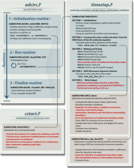
Chapter 2 – ADCIRC Background ... 3
2.1 ADCIRC Formulation ... 3
2.2 Wetting and Drying Algorithm ... 4
2.2.1 Initialization of Wetting and Drying ... 5
2.2.2 Wetting and Drying Criteria ... 5
2.3 Parallel ADCIRC ... 6
Chapter 3 – Improvements in Subdomain Modeling ... 9
3.1 Wet/Dry Forcing in Subdomain Modeling... 9
3.1.1 LTSA Model of Wetting and Drying Algorithm ... 9
3.1.1.1 Node ... 11
3.1.1.2 Elements ... 13
3.1.1.3 Algorithm ... 14
3.1.1.4 Parallel Composition ... 19
3.1.2 Analysis of LTSA Model of Wetting and Drying Algorithm ... 22
3.2 Methodology ... 23
3.3 Frequency of Forcing ... 26
3.4 Packaging ... 26
3.5 Example Problems ... 27
3.5.1 Quarter Annular Test Case ... 27
3.5.2 Hurricane Fran – Cape Fear Region ... 28
3.5.3 Hurricane Isabel – Cape Hatteras Region ... 33
Chapter 4 – Subduration Modeling ... 36
4.1 Hot-Starting in ADCIRC ... 36
4.2 Implementation of Subduration Modeling ... 36
4.3 Modifications Made to the Hot-start Algorithm ... 37
4.4 Test Case – Levee 1 ... 38
4.5 Test Case – Levee 2 ... 40
Chapter 5 – Conclusions ... 42
APPENDICES ... 45
Appendix A – Subdomain User's Guide ... 46
A.1 Work Flow of Subdomain Modeling ... 46
A.2 Descriptions of Subdomain Modeling files and parameters ... 48
A.3 Subdomain Modeling User’s Guide ... 49
Appendix B – Subdomain Changes Made in ADCIRC Code ... 57
Appendix C – Additional LTSA Diagrams ... 73
Appendix D – Trace-to-violations of LTSA Model properties ... 75
D.1 Trace to property violation in Subdomain1 ... 75
D.2 Trace to property violation in Subdomain2 ... 76
Appendix E – Model Parameter and Boundary Condition Files (fort.15) ... 77
E.1 Hurricane Fran Subdomain Runs ... 77
LIST OF TABLES
Table 3.1: Descriptions of the states of the process NODE. ... 13
Table 3.2: Maximum values and absolute errors of quarter annular problem. ... 28
LIST OF FIGURES
Figure 2.1: Maximum elevation comparison between serial run and 4-processor parallel run. ... 7
Figure 2.2: Maximum elevation comparison between serial run and 8-processor parallel run. ... 7
Figure 2.3: Maximum elevations comparison between serial run and 40-processor parallel run. ... 8
Figure 2.4: Absolute errors of Parallel ADCIRC runs using various number of processors. ... 8
Figure 3.1: LTSA drawing of a process NODE. ... 10
Figure 3.2: A basic LTSA model of a node. ... 10
Figure 3.3: Representations of Grids Modeled in LTSA. ... 11
Figure 3.4: LTSA model of the process NODE. ... 12
Figure 3.5: LTSA Diagram of the process NODE. (Output actions are omitted.). ... 12
Figure 3.6: LTSA model of the process ELEMENT. ... 13
Figure 3.7: LTSA Diagram of the process ELEMENT. ... 14
Figure 3.8: LTSA model of the process PART1. ... 15
Figure 3.9: LTSA model of the process PART2. ... 15
Figure 3.10: LTSA model of the process PART3. ... 16
Figure 3.11: LTSA model of the process MJU.. ... 17
Figure 3.12: LTSA model of the process PART4. ... 17
Figure 3.13: LTSA model of the process UPDATE. ... 18
Figure 3.14: LTSA model of the process REPORTNODES. ... 18
Figure 3.15: LTSA model of the process INITIALIZATION. ... 18
Figure 3.16: LTSA model of the process PART0. ... 19
Figure 3.17: LTSA model of the process SEQUENCE. ... 19
Figure 3.18: Modified LTSA model of the process PART1. ... 20
Figure 3.19: Parallel composition of the model of wetting and drying algorithm. ... 21
Figure 3.20: LTSA models of elemental properties.. ... 21
Figure 3.21: LTSA model of property Subdomain1.. ... 22
Figure 3.22: LTSA model of property Subdomain2. ... 22
Figure 3.23: Flowchart of the modified subdomain modeling approach. Adapted from Tanaka et al. (2010). ... 24
Figure 3.24: Timestepping scheme of subdomain modeling. (Modifications made to the original ADCIRC code are in red.). ... 25
Figure 3.25: Subdomain modeling applied to the quarter annular problem. ... 27
Figure 3.27: Subdomain grid consisting of 28,643 nodes and 56,983 elements. ... 30
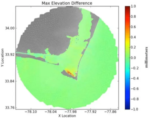
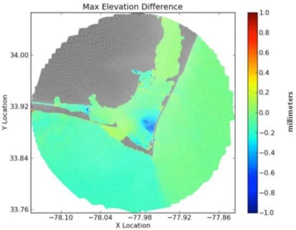
Figure 3.28: Hurricane Fran – Cape Fear, Maximum elevation differences at various forcing intervals. (a) N = 3600 timesteps, (b) N = 1600 timesteps, (c) N = 800 timesteps, (d) N = 100 timesteps. ... 31
Figure 3.29: Hurricane Fran – Cape Fear, Maximum elevation differences at various forcing
frequencies. (a): 0-100%, (b): 93-100%. ... 32
Figure 3.30: Hurricane Fran – Cape Fear, Maximum velocities comparison (Subdomain forced every 100 timesteps). ... 33
Figure 3.31: Elliptical Cape Hatteras Subdomain Grid. ... 34
Figure 3.32: Hurricane Isabel – Cape Hatteras, Maximum elevation differences.. ... 35
Figure 4.1: Initial states of a cold-started Model. (a) Bathymetric depth, (b) Surface Elevation, (c) Total water height.. ... 37
Figure 4.2: (a) Hot-started Subdomain grid, (b) Area flooded during a cold-started run, (c) Levee added to hot-started run. ... 39
Figure 4.3: Maximum Elevation Comparison between hot-started and cold-started run. ... 39
Figure 4.4: Modified subdomain grid of Test Case - Levee 2. ... 40
Figure 4.5: Maximum Elevation Comparison between hot-started and cold-started runs of Test Case – Levee 2. ... 41
Figure A.1: Summary of the work flow of Subdomain Modeling Approach. ... 47
Figure A.2: Quarter Annular Test Grid. ... 53
Figure C.1: LTSA Diagram of the process PART1: If the water level of the wet node is greater than H0, the node stays wet (trace: 0, 1, 0). If the water level is less than H0, node is dried (trace: 0, 2, 3, 0). Hidden actions: part1.start, part1.end, node[1].update_nc. ... 73
Figure C.2: LTSA Diagram of the process PART2. If the velocity is greater than Vmin, nodes in the element are made wet (trace 0, 2, 3, 4, 5, 0). Minimization Operator: PART2@{ele[1].evaluate, ele[1].node[i:1..3].wet_node,velmin,v_gt_velmin,v_le_velmin}. ... 73
Figure C.3: LTSA Diagram of the process PART3. (Trace 0, 1, 2, 0: Element has less than two wet nodes, element is dried. Trace 0, 3, 4, 2, 0: Element has at least two wet nodes, h < Hoff. Element is dried. Trace 0, 3, 4, 5, 0: Element has at least two wet nodes, h ≥ Hoff. Element is wetted.
Minimization operator: PART3@{ele[1].{evaluate3,dry_element,wet_element},hoff}). ... 74
Chapter 1 – Introduction
The vulnerability of coastal areas to storm surge has led scientists and engineers to develop methods
that predict and analyze the effects of hurricanes, which may result in loss of human life and property.
Storm surge modeling is a powerful computational method of forecasting inundation caused by
potential hurricanes. It is widely used by civil engineers to examine the performance of civil
infrastructure and to design hurricane resistant structures in coastal regions. To obtain sufficient
information from a storm surge model, it is often necessary to consider multiple storm surge and
flooding scenarios. Consequently, storm surge models are expected to provide reliable information
and to perform efficiently.
In order to capture the natural characteristics of hurricane storm surge realistically, computational
models are generally required to cover large domains using high resolution grids, increasing the
computational requirements to perform such simulations (Luettich, Westerink & Scheffner, 1992).
This research presents two approaches, subdomain modeling and subduration modeling, that improve
the efficiency of storm surge simulations when various inundation scenarios are to be examined.
These approaches are implemented in ADCIRC, a finite element based storm surge model widely
used by the US Army Corps of Engineers, FEMA, and others. The basic formulation of ADCIRC and
its wetting and drying algorithm, which has an impact on the approach taken and on the accuracy of
ADCIRC itself, are presented in Chapter 2.
The subdomain modeling approach, originally introduced by Simon and Baugh (2011), is based on
forcing the data of boundary nodes of a smaller grid within the original, larger grid. The approach is
used to reduce the total runtime of a series of hurricane storm surge simulations where alternative
topographies and configurations in a geographical region of interest are examined. Improvements in
the approach are presented in Chapter 3, where finite state models of ADCIRC’s wetting and drying
algorithm reveal an interaction with the subdomain approach that must be accommodated. Additional
enhancements are presented that increase the accuracy and accessibility of the approach, and test
In Chapter 4, the subduration modeling approach is presented for downscaling hurricane storm surge
models in time. The hot-start feature of ADCIRC is a capability allowing the restart of a simulation at
a particular timestep. This feature is drawn upon to reduce the runtime of a series of simulations when
various local changes to the terrain are applied. The changes made to the hot-start algorithm and
several test cases are presented.
Finally, conclusions are presented in Chapter 5, and a user’s guide for the modified subdomain
Chapter 2 – ADCIRC Background
ADCIRC is a storm surge model widely used by scientists and engineers to analyze the effects of
hurricanes on coastal regions. ADCIRC performs with high accuracy and efficiency as a result of
numerical algorithms, optimization of governing equations, and extreme grid flexibility (Luettich,
Westerink & Scheffner, 1992). An ADCIRC run can be performed in serial or in parallel, and
hydrodynamic equations can be solved with two-dimensional depth-integrated (2DDI) or
three-dimensional equations.
2.1 ADCIRC Formulation
For the ADCIRC-2DDI, the version used throughout this research, the equation solved to determine
the water surface elevation is the Generalized Wave Continuity Equation (GWCE), and the equation
solved to determine the depth-averaged velocity is the vertically-integrated momentum equation
(Luettich & Westerink, 2004). The GWCE is derived from the primitive depth-integrated continuity
equation and the primitive depth-integrated conservation of momentum equations, which lead to a
discrete system of equations (Luettich et al., 1992).
Numerical discretization in time is performed using finite differences (Luettich et al., 1992). Time
discretization of the GWCE using the finite difference method is achieved by implementing a
variably weighted, three-time-level scheme, while the time discretization of momentum equations is
achieved by implementing a two-time-level variably weighted scheme (Luettich et al., 1992). Finally,
numerical discretization in space is performed using the finite element method to complete the
conversion of the governing equations into algebraic equations (Luettich et al., 1992). Three-node
linear triangular elements, which have proved to be flexible and cost-effective, are used for finite
element discretization (Luettich et al., 1992).
After fully discretizing the GWCE, the following global system of equations is obtained (Luettich et
where
N: number of nodes
: the global banded system matrix
: the global load vector
: the global nodal elevation vector
After fully discretizing the momentum equations, the following global system of equations is
obtained (Luettich et al., 1992):
where
= global diagonal system matrices
= global right-hand-side load vectors,
= global velocity vectors in the x and y directions
2.2 Wetting and Drying Algorithm
The wetting and drying algorithm in ADCIRC is used to determine whether nodes and elements
inside the grid should be activated or deactivated within a timestep (Luettich & Westerink, 1995).
Activated (wet) areas inside the grid are included in hydrodynamic calculations while deactivated
(dry) areas are excluded from the calculations (Luettich & Westerink, 1995).
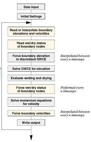
In an ADCIRC timestep, the wetting and drying algorithm appears after the solution of the continuity
equation and before the solution of the momentum equation (Dietrich, Kolar & Luettich, 2004).
particularly important to be mindful of its effects both on the approach used for subdomain modeling
and on the accuracy and stability of ADCIRC itself.
2.2.1 Initialization of Wetting and Drying
The wetting and drying algorithm in ADCIRC is controlled by three variables: (1) nnodecode
maintains the wet/dry status of a node and is updated frequently within the wet/dry algorithm in a
timestep. (2) nodecode maintains the wet/dry status of a node, but is updated after the wetting and
drying algorithm is completed. (3) noff maintains the wet/dry status of an element. These variables
are initialized in accordance with the bathymetry of the grid and the configuration of the model:
- Nodes that have less water height than H0 (minimum water depth) are initialized as dry nodes and the surface elevation of these nodes are set to H0-DP(DP: bathymetric depth). Remaining nodes are initialized as wet nodes. However, if a node is configured to be dry (a user-defined setting),
ADCIRC will initialize the node as dry, even though it is below mean sea level.
- If a wet node is connected to dry nodes only, the node will be initialized as a dry node
(landlocking).
- All the elements are set to be wet at the beginning of the simulation unless it is hot started.
2.2.2 Wetting and Drying Criteria
Several criteria are applied on the grid to specify the states of nodes and elements. The wetting and
drying criteria taken from the ADCIRC source code (Version 50.51) are as follows:
- First, the water surface elevations of the nodes are checked to determine whether they are greater
than H0; the minimum water depth for a node to be considered wet. If the water height is greater than H0, the node remains wet. Otherwise, the node becomes dry and is excluded from the hydrodynamic calculations.
- Second, a nodal wetting criterion is applied on the elements when a node is dry but the rest of the
nodes are wet. If the water column heights of both wet nodes are greater than or equal to Hoff = 1.2xH0, and if the water level of the dry node is less than the water level of one of the wet nodes, the dry node is made wet if the steady state velocity is greater than Vmin (Dietrich et al., 2004). - Third, an elemental drying criterion is applied. If one of the two nodes with higher water surface
- Finally, wet nodes that are only connected to dry elements are dried.
After the implementation of the wetting and drying algorithm, the wet/dry states of the nodes and
elements are updated within the timestep.
2.3 Parallel ADCIRC
ADCIRC can be run in parallel on computer clusters to reduce the computing time of a large model.
Decomposition of the domain for a parallel ADCIRC run is done using METIS (Karypis and Kumar,
1998), and Message Passing Interface (MPI) is used for communication between each processor.
Message passing between neighboring subdomains is done using a communication layer: data of the
inner nodes is sent to neighboring subdomains and data of the outer nodes is received from the
neighboring subdomains (Tanaka et al., 2010). Additionally, a global communication is performed
among all processors to calculate the dot product in the iterative solver (Tanaka et al., 2010).
To demonstrate the effects of parallelization on accuracy of ADCIRC, an example problem is run on
a large domain containing 620,089 nodes and 1,224,714 elements. A serial run and several parallel
runs using different numbers of processors are performed. These runs are compared on a small,
circular area containing 28,643 nodes. The maximum surface elevations of the nodes for each run are
compared. Maximum elevation comparison plots show that parallel ADCIRC introduces small
deviations from the serial simulation (Figures 2.1, 2.2, and 2.3). In addition, an error convergence plot
(Figure 2.4) shows that increasing the number of the cores used in a parallel run exacerbates these
deviations.
It is observed that the divergence between serial and parallel solutions, which is negligible in most
cases, is caused by the iterative solver and the precision of the MPI library. These errors appear to be
occurring at regions of complex topography. Although the differences between serial and parallel
runs are negligible during the initial timesteps of the model, they accumulate and eventually result in
Figure 2.1: Maximum elevation comparison between serial run and 4-processor parallel run
Figure 2.3: Maximum elevations comparison between serial run and 40-processor parallel run
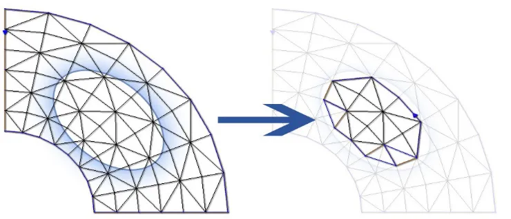
Chapter 3 – Improvements in Subdomain Modeling
Subdomain modeling in ADCIRC reduces the total runtime of a series of hurricane storm surge
simulations to be performed for a particular storm on multiple, alternative topographies in a
geographical region of interest. The approach is based on forcing the data of boundary nodes of a
considerably smaller grid called a subdomain within the original, larger grid. Boundary conditions of
subdomains are obtained from the output files of an original full run and are then used as input files
for the subdomain runs. Boundary node data of subdomains are enforced once they are read from
input files at specified time intervals, and are linearly interpolated at intermediate timesteps.
Approaches designed to improve the accuracy and accessibility of the technique are described below.
3.1 Wet/Dry Forcing in Subdomain Modeling
The approach to subdomain modeling originally outlined by Simon (2011) enforces only elevations
and velocities as boundary conditions and omits the wet/dry states of boundary nodes due to their
ineligibility for interpolation and the concomitant increase in secondary storage. In the following
sections, the effects of the wetting and drying algorithm on subdomain modeling are described, and
wet/dry forcing is then introduced in ADCIRC to improve the fidelity of the approach.
3.1.1 LTSA Model of Wetting and Drying Algorithm
In this section, ADCIRC’s wetting and drying algorithm is modeled as a finite state machine to look
for potential conditions under which the wet/dry states of boundary nodes may fail to be properly
determined in a subdomain model. The presence of such conditions would imply that wet/dry states
along a subdomain boundary cannot simply be recomputed from available information within a
subdomain run and must therefore be saved from a full run and subsequently imposed on the
boundaries of a subdomain. LTSA, a finite state model-checking tool (Magee and Kramer, 2006), is
LTSA Background:
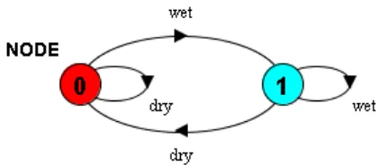
LTSA is a model checking tool that supports the representation and analysis of finite state systems.
Actions in LTSA denote a transition between states and are depicted as arcs between nodes. In Figure
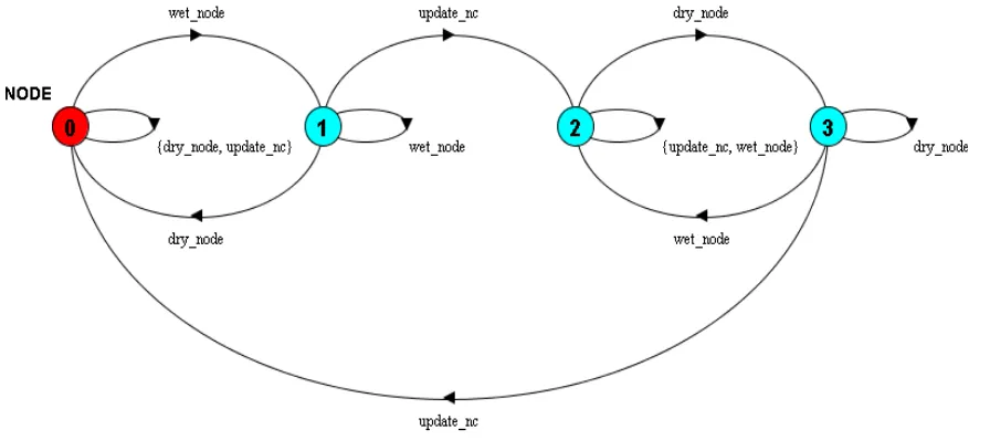
3.1, the dry action causes a node to become (or stay) dry (State 0). Likewise, the action wet causes a node to become (or stay) wet (State 1). In LTSA, this graphical representation is defined as a process,
NODE, using a syntax comparable to other process algebraic languages, as shown in Figure 3.2. The
expressive power of the language is enhanced through the use of indexing, which may be applied to
both processes and actions.
Figure 3.1: LTSA drawing of a process NODE.
Figure 3.2: A basic LTSA model of a node.
In this particular case indexing of the NODE process results in the following expected unfolding:
NODE[0] = ( wet -> NODE[1] | dry -> NODE[0] NODE[1] = ( wet -> NODE[1]
| dry -> NODE[0]).
Wetting and Drying Model:
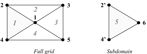
The LTSA model of wetting and drying described below consists of six nodes and five elements.
These nodes and elements form two basic grids, as shown in Figure 3.3. The first grid models a full
domain consisting of four elements and the second grid models a subdomain, which is the equivalent
of element 1 in the full domain, and node 6 in the subdomain corresponds to node 1 in the full
domain.
Full grid Subdomain
Figure 3.3: Representations of grids modeled in LTSA
3.1.1.1 Node
First, the behavior of a node in a grid is modeled. Since a node in ADCIRC uses two variables to
designate its wet/dry status, nnodecode and nodecode, the process NODE in the LTSA model similarly has two indices: nnc and nc. The actions wet_node and dry_node signal the transition of the wet/dry status of a node. When the status of a node is changed by these actions, the index nnc is set accordingly. The action update_nc updates the nodecode. The actions is_wet and
is_dry are used as output actions by subsequent processes. It should be noted that the process NODE is labeled with the set of nodes to disjoin the alphabets of all six nodes. Prefixing is used to label each action in the process with the number of the node. For example, the action wet_node of the third node is transformed into node[3].wet_node.
2’
4’
6
5
2
1
2
3
4
5
3
1
Figure 3.4: LTSA model of the process NODE.
Descriptions of variables used in the LTSA model of the NODE process: NP: number of nodes in the model.
Nodes: set of nodes.
NodesAlpha: action alphabet of the process NODE.
Table 3.1: Descriptions of the states of the process NODE.
nnc nc Description
State 0: 0 0 Node is dry.
State 1: 1 0 Node is wet, but not yet updated.
State 2: 1 1 Node is wet.
State 3: 0 1 Node is dry, but not yet updated.
3.1.1.2 Elements
In similar fashion, the behavior of an element can be modeled. The index nf represents the wet/dry status of an element. The actions wet_element and dry_element signal the transition of the wet/dry status of the element. The actions is_wet_ele and is_dry_ele are used as output actions by remaining processes. The process ELEMENT is also prefixed with the set of elements to disjoin the alphabets of all five elements.
Figure 3.6: LTSA model of the process ELEMENT.
Descriptions of variables used in the LTSA model of the ELEMENT process: NE: number of elements in the model.
Elements: set of elements.
Figure 3.7: LTSA Diagram of the process ELEMENT.
3.1.1.3 Algorithm
The wetting and drying algorithm in ADCIRC consists of four main criteria as described in section
2.2.2. Each criterion is separately modeled and a parallel composition of nodes, elements, and parts of
the algorithm is performed to complete the model. Minimized LTSA diagrams of the components of
the wetting and drying algorithm are provided in Appendix C.
PART1: If the total water height of a wet node is less than H0, the node is made wet and updated. First, the process is initiated when the action part1.start is signaled. Wet/dry states of the nodes are sequentially determined using synchronized output actions; is_wet or is_dry. The index n of subprocess PART1_main represents the node numbers and is also used to determine the end of the process. When the node is dry, the process skips to the next node; n+1. If the node is wet, a
Figure 3.8: LTSA model of the process PART1.
PART2: If an element has two wet nodes, and if the steady state velocity is greater than Vmin (represented with the action v_gt_velmin), the third dry node of the element is also made wet. First, the number of the wet nodes of an element is counted in subprocess PART2_main using the synchronized actions; is_wet and is_dry. The index nctot of PART2_main is increased by one if a node inside an element is determined to be wet, and the index is passed to PART2_eval to evaluate the element. Then, the steady state velocities of elements having two wet nodes are
non-deterministically chosen to be greater or less than Vmin in the subprocess PART2_eval. If the velocity is greater than Vmin, it is ensured that all the nodes of the elements are wet. Otherwise, the process skips to next element. When the index e exceeds the number of elements of the model (when
(e==NE+1)), the process engages in only available action part2.end, and returns to the beginning for the evaluation of the next timestep.
It should be noted that the nodal actions are prefixed with the elements to imply the assembly of the
grid. For example, node[5].wet_node action of node 5, which is the second node of element 3, is represented by ele[3].node[2].wet_node (to complete the assembly, relabeling is implemented in the composite process: node[5]/ele[3].node[2] ).
PART3:The number of wet nodes in an element is counted in the subprocess PART3_main as is done in PART2_main. If an element has only one wet node, the element is taken to be dry. If two or more nodes of an element are wet, a non-deterministic choice is made in the subprocess
PART3_eval: h is defined to be either greater or less than Hoff.
Figure 3.10: LTSA model of the process PART3.
PART4: The land-locking criterion is applied: if a wet node is not connected to an active (wet) element, the node is dry. To implement this criterion, an additional process called MJU is introduced. This process maintains an index mju for each node in the model. If the node is connected to at least one wet element, the index mju is set to 1. The alphabet of the process is synchronized with the process PART4. Note that this process is also prefixed with the set of nodes for synchronization.
index mju of a node n is previously set to 1, the process engages in only eligible action node[n].has_active_ele. After the occurrence of this action, node[n].reset action is signaled to reset the index mju of the node for the next timestep. However, if the node does not have any active element, only eligible action left is node[n].no_active_ele. This action is followed by node[n].landlocking, which eventually results in drying of the node.
Figure 3.11: LTSA model of the process MJU.
Figure 3.12: LTSA model of the process PART4.
Figure 3.13: LTSA model of the process UPDATE.
REPORTNODES: This process is added to simplify the analysis. The actions report_wet or report_dry are signaled depending on the state of the node.
Figure 3.14: LTSA model of the process REPORTNODES.
INITIALIZATION: This process is implemented to initialize the nodes of the model at the beginning of the execution. The nodes are started either dry or wet, and updated. When the
initialization ends, the process moves to subprocess IDLE and waits until the end of the execution.
Figure 3.15: LTSA model of the process INITIALIZATION.
PART0: This process is implemented to initialize the elements of the model at the beginning of a timestep. Elements of the model are started wet, as is done ADCIRC code. After the end of the
Figure 3.16: LTSA model of the process PART0.
3.1.1.4 Parallel Composition
Finally, the processes are combined using the parallel composition operator. In ADCIRC, the parts of
the wetting and drying algorithm in a timestep are executed in sequence. However, a concurrent
LTSA model operates interleaved and asynchronous (Magee and Kramer, 2006). To ensure that the
processes are sequentially executed, an additional process called SEQUENCE is implemented.
Figure 3.17: LTSA model of the process SEQUENCE.
Since start and end actions of all the parts are synchronized and put in order with this process, it is ensured that the processes are executed in the desired sequence.
Another problem of parallel composition results from synchronized actions. Shared actions are
required to occur at the same time in all the processes. However, the wetting and drying algorithm in
a timestep is sequential, which means that only one participant of the algorithm is active at a time.
Since the other processes are not yet started, they cannot engage in shared actions. For instance, if the
process PART1 is required to engage in the action node[1].dry_node, all other constituent processes sharing the action are also required to participate in it, which is not possible since they
To overcome this problem, modifications are made to all constituent processes of the sequential
procedure: PART0, PART1, PART2, PART3, PART4, UPDATE, REPORTNODES. These modifications are:
1. Add the action idle as an alternative of the action start.
2. Using a relabeling function, replace the action idle with the actions in the alphabets of the processes NODE and ELEMENT.
For example, the process PART1 is modified as shown in Figure 3.18.
Figure 3.18: Modified LTSA model of the process PART1.
These modifications ensure that, when the processes forming the sequential algorithm are not yet
started, they do not restrain the active process from engaging in shared actions in the alphabets of
NODES or ELEMENTS.
The parallel composition of the entire model is shown in Figure 3.19. As mentioned, a relabeling
function is used to assemble the grids of the model. Idle actions, which are replaced with the
alphabets of nodes and elements, can occur anytime during the execution. To restrain the model from
arbitrary occurrences of these actions, the alphabets of nodes and elements are given lower priority.
The composite process has 96,039 states for a model comprised of five elements and six nodes, and
results in no deadlock. In addition to deadlock analysis, a basic safety analysis is performed using two
nodes cannot be wet. The property Check_Element2 states that if an element is wet, the nodes connected to it should have an active element. Since the ERROR states for both properties are
unreachable, no violation is detected.
Figure 3.19: Parallel composition of the model of wetting and drying algorithm
3.1.2 Analysis of LTSA Model of Wetting and Drying Algorithm
First, one of the possible faulty traces due to the lack of forcing wetting and drying in the subdomain
approach is revealed by implementing the property Subdomain1. This property leads to an error when
node 1 is wet and node 6 is dry. Examining the trace-to-violation of this property, it is observed that
when node 1 is wet, node 6 is dry due to land locking. Node 1 has three other elements connected,
which can prevent it from land locking when element 1 is dry. However, since node 6 is connected to
only one element (which may occur on boundary nodes of subdomains regardless of the size of the
grid), it is dry due to land locking whenever element 5, which is the equivalent of element 1, is dry.
Figure 3.21: LTSA model of property Subdomain1.
Another possible faulty trace is revealed using the property Subdomain2. This property leads to error
when node 1 is dry and node 6 is wet. Examining the trace to violation of this property, it is observed
that even small differences in water height and velocity of boundary elements may result in different
wet/dry states, which could potentially magnify the divergence of solutions obtained for a subdomain
when compared with those of the full domain.
These results imply that the wet/dry states of nodes and elements just outside of a subdomain are
needed by ADCIRC’s wet/dry algorithm to faithfully reproduce wet/dry states within a subdomain.
By recording and later enforcing these states on the boundary of a subdomain, however, the algorithm
has sufficient boundary information in the context of a subdomain run to reproduce the states found in
a full run.
3.2 Methodology
As shown in the previous section, the wetting and drying of nodes on the boundaries of subdomains
must be recorded from full runs and then enforced in subdomain runs to ensure the accuracy of the
approach. The boundary nodes of subdomains are assigned as “elevation specified” boundary nodes
(NBFR=0 & NOPE>0), and non-periodic elevation boundary condition file, which is previously extended to include velocity (Simon, 2011), is now extended also to include wet/dry status of the
boundary nodes. Flow across the “elevation specified” boundary nodes is allowed.
Since ADCIRC output reports the elevation and velocity of nodes, that information may be
conveniently obtained from full runs to create input files (boundary conditions) for subdomain runs.
Wet/dry states, on the other hand, are generally not reported, so ADCIRC must be modified to report
them at specified time intervals. Having obtained the wet/dry states of nodes in a full-scale run, the
content of the boundary conditions is extended by adding these states to the input files of subdomains.
Finally, ADCIRC code for a subdomain run is modified to read in the states of the boundary nodes
and to enforce wetting and drying to ensure that the subdomain boundary nodes have the same
wet/dry states as the corresponding nodes in the full-scale run. Since it is impossible to interpolate
between binary states, they are instead forced to remain the same until the next timestep when reading
the next collection of boundary conditions occurs. By increasing the forcing frequency, as
subsequently described, it is possible to eliminate potential inconsistencies caused by the need to
interpolate. The complete list of the modifications made in ADCIRC source code is provided in
Appendix B. Flowchart of the modified subdomain modeling approach is shown in Figure 3.23. In
addition, a diagram that summarizes the modifications made to ADCIRC code is shown in Figure
3.3 Frequency of Forcing
Another improvement introduced for subdomain modeling is to increase the frequency at which
boundary conditions are enforced. In our original implementation, writing the output of all the nodes
in a grid at high frequency required large amounts of secondary storage and decreased the runtime
performance of ADCIRC. In order to overcome these problems, the output scheme of the simulation
is slightly changed: (1) Instead of reporting all node data in full-scale run, only those nodes on the
boundaries of subdomains are written to output files. (2) An additional set of output files is introduced
to report the data of anticipated subdomain boundary nodes, so that the original set of output files is
reserved for use in examining the entire full run. These modifications enable the subdomain modeling
approach to have a higher frequency of forcing without having a significant decrease in ADCIRC
runtime performance or an increase in secondary storage. As such, it is possible to eliminate the
errors caused by potential instabilities of low frequency wet/dry forcing and linear interpolation of
elevation and velocity.
3.4 Packaging
In order to increase the practicality of the subdomain approach, several changes have been made to
the implementation. The approach is reduced to four main steps: (1) Generate subdomain and full
domain control file, (2) Run ADCIRC on the full domain, (3) Extract subdomain boundary
conditions, (4) Run ADCIRC on the subdomain. Only two of these steps are new to ADCIRC, and
these are automated with additional scripts so that users are only required to input the parameters of
the subdomain model. Adjustability of the approach is also improved by allowing users to configure
the boundary forcing of subdomains.
Using this new subdomain approach, ADCIRC now checks for the existence of a subdomain
modeling control file at startup. If the file exists, subdomain modeling features are activated.
Otherwise, ADCIRC runs normally, ensuring that conventional runs are unaffected. In addition, the
data of a full run used to create the boundary conditions of a subdomain are written to a different set
3.5 Example Problems
In this section, several test cases are presented to confirm that the modified subdomain modeling
approach is capable of downscaling hurricane storm surge models accurately, allowing engineers to
assess a variety of test case scenarios in a considerably shorter runtime and using less secondary
storage.
3.5.1 Quarter Annular Test Case
The quarter annular test case, first developed by Lynch and Gray (1978), is a simple example
commonly used to evaluate the performance of numerical approaches for solving hydrodynamic
problems (Westerink, Luettich & Scheffner, 1994). The ADCIRC model of this problem consists of
63 nodes and 96 elements, as shown in Figure 25. The outside arc of the grid is an open ocean
boundary, which is subject only to tidal forces, and the inside arc is a land boundary that reflects the
tidal forces.
Figure 3.25: Subdomain modeling applied to the quarter annular problem
An elliptical subdomain consisting of 16 nodes and 18 elements is created from the original quarter
and wet/dry states of the boundary nodes obtained from the original run is created and used to enforce
the subdomain grid. It is observed that the maximum difference between maximum water surface
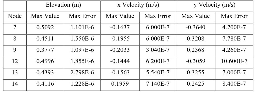
elevations of a node located in both grids is 2.8x10⁻⁶ m. Therefore, results obtained from the quarter annular test case confirm the accuracy of subdomain modeling approach.
Table 3.2: Maximum values and absolute errors of quarter annular problem
Elevation (m) x Velocity (m/s) y Velocity (m/s)
Node Max Value Max Error Max Value Max Error Max Value Max Error
7 0.5092 1.101E-6 -0.1637 6.000E-7 -0.3640 4.700E-7
8 0.4511 1.550E-6 -0.1955 6.000E-7 0.3208 7.780E-7
9 0.3777 1.097E-6 -0.2033 3.040E-7 0.2368 4.260E-7
12 0.4996 1.855E-6 -0.1444 6.200E-7 -0.3059 10.600E-7
13 0.4393 2.798E-6 -0.1563 5.540E-7 0.3255 7.000E-7
14 0.4116 1.228E-6 0.1959 7.140E-7 0.2425 8.400E-7
3.5.2 Hurricane Fran – Cape Fear Region
To demonstrate the scope of application and accuracy of the approach, a physically realistic storm
surge event on a large grid located along the Atlantic coast of North America is studied. To be able to
properly reflect the physical aspects of storm surge of Hurricane Fran, the original grid covers a large
geographical area along the Atlantic coast from Venezuela to Nova Scotia, as shown in Figure 3.26.
A significantly smaller grid inside the original grid is created as a subdomain in the Cape Fear region,
as shown in Figure 3.27. As previously studied by Simon (2011), the aim of this example is to make
the subdomain modeling approach available for engineers to examine various inundation scenarios, to
investigate the effects on existing civil infrastructure, and to make engineering decisions that better
Figure 3.26: Full grid consisting of 620,089 nodes and 1,224,714 elements
3.5.2.1 Model Setting
A circular subdomain consisting of 28,643 nodes and 56,983 elements is generated from a full grid
consisting of 620,089 nodes and 1,224,714 elements. The model type is a barotropic 2DDI run.
Nodal attributes are: surface directional effective roughness length, canopy coefficient, Manning’s n
at sea floor, primitive weighting in continuity equation, and average horizontal eddy viscosity in the
sea.
The total simulated runtime of the model is 3.9 days using a timestep of 0.5 seconds. The minimum
water height for a node to be considered wet is 0.1 m and the minimum velocity is 0.01 m/s. The
subdomain has 302 boundary nodes that are forced every 100 timesteps (50 seconds). First, a full run
on the original grid is performed. The output files of the full run are used to create the boundary
conditions file of the subdomain grid. Then, a subdomain run is performed and the results are
Figure 3.27: Subdomain grid consisting of 28,643 nodes and 56,983 elements
Full Domain Specifications:
NC FEMA Mesh Version 9.92, ADCIRC Version 50
Model Type: Barotropic 2DDI / GWCE, Momentum equation
Subdomain Specifications:
Radius: 10.8 miles, Area: 366.5 sq miles
3.5.2.2 Analysis
By using subdomain modeling, 600 CPU-hours of runtime are reduced to 40 CPU-hours. The
maximum water elevations of the full domain and the subdomain are compared. It is observed that the
largest elevation difference occurring in a node is 3.6 millimeters, and that 99.7% of the nodes have
differences less than a millimeter. The maximum water velocities are also compared, and it is seen
that only one node has a maximum velocity difference exceeding 0.3 m/s. Referring back to the
original problem (Simon, 2011), where several nodes had elevation differences exceeding 15 cm and
velocity differences exceeding 1.5m/s, it is concluded that modifications made in the subdomain
Additionally, the effect of the boundary forcing frequency on the accuracy of the subdomain
modeling is examined. Here, the same subdomain run is performed with various N values (timestep
intervals at which the boundary conditions are read from the subdomain input file), and the results are
compared to a full run. As can be seen from Figure 3.28 and Figure 3.29, the accuracy of the
approach improves with forcing frequency.
(a) (b)
(c) (d)
(a)
(b)
Figure 3.30: Hurricane Fran – Cape Fear, Maximum velocities comparison (Subdomain forced every 100 timesteps).
3.5.3 Hurricane Isabel – Cape Hatteras Region
Another realistic storm surge event, Hurricane Isabel is studied to evaluate the accuracy of the
modified subdomain approach. The full grid used in the previous example is also used as the original
grid in this problem. The Cape Hatteras region, located on the North Carolina coast, is selected as the
subdomain location. In contrast with the example presented by Simon (2011), an elliptical subdomain
is defined as shown in Figure 3.31.
3.5.2.1 Model Setting
An elliptical subdomain consisting of 8,248 nodes and 16,310 elements is generated from the original
185 boundary nodes that are forced every 100 seconds. The remaining model parameters are the same
as the previous example.
Figure 3.31: Elliptical Cape Hatteras Subdomain Grid
3.5.2.2 Analysis
Results obtained from the Hurricane Isabel full run are used to enforce the subdomain boundary
conditions. By using subdomain modeling, 400 CPU-hours of runtime are reduced to 7 CPU-hours.
Maximum water surface elevations of the original run and the subdomain run are compared to
evaluate the accuracy of the approach. It is seen that the largest elevation difference occurring in a
node is 10 cm and only 4 nodes have maximum elevation error greater than 1 cm. In addition,
maximum velocities are compared. It is observed that only 5 nodes have maximum velocity error
larger than 0.5 m/s. It is confirmed that modified subdomain modeling approach enables engineers to
Chapter 4 – Subduration Modeling
Subduration modeling in ADCIRC is introduced as a means of downscaling hurricane storm surge
models in time. The hot-start feature of ADCIRC, which allows users to begin a run from a specified
timestep using initial conditions obtained from a previously performed run, is used to reduce the total
runtime of series of simulations where users have made topographic or other changes to a model. This
chapter describes the hot-start feature of ADCIRC as well as its use in reducing computation time
when certain changes need to be made to a simulation and then re-run. The approach and scope of
changes that can be addressed in this manner are described, and several test cases are presented.
4.1 Hot-Starting in ADCIRC
A conventional use of the hot-start feature in ADCIRC is to restart a simulation in the event of a
computer failure during a run (Westerink, Luettich & Scheffner, 1994). When the feature is
activated, the data of the entire grid —including water surface elevation, depth-averaged velocity, and
wet/dry flags— are recorded at specified timesteps in two hot-start files on an alternating basis.
Recording hot-start files in this way ensures that at least one of the files is written successfully
(Westerink et al., 1994). Once a simulation is hot-started, ADCIRC reads the data of the grid from the
hot-start input files, and starts the model from the timestep when the latest hot-start file is written.
4.2 Implementation of Subduration Modeling
By making use of the hot-start feature of ADCIRC, it is possible to skip calculations of a model until
some specified timestep. Doing so can save significant amount of runtime especially when the runs
are performed repeatedly. This method can be used to change model parameters of a run at a
particular timestep. In addition, topographic changes can be made in order to examine different
design and failure scenarios. A potential hurdle, however, is that ADCIRC does not allow users to
change the grid information file if the model is hot-started. In other words, grid information files of
To further describe the problem, a simple terrain is used to illustrate the basic concepts of hot-starting
in ADCIRC. Figure 4.1 represents the state and the properties of a cold started model at the initial
stage. DP, shown as the green curve in Figure 4.1.a, is the bathymetric depth of a node with respect to
the geoid, and is positive below the geoid. ETA is the surface elevation of a node and is shown as the
red curve in Figure 4.1.b. It is positive above sea and zero at mean sea level. HTOT is total water
height and is calculated by adding DP to ETA. It is shown as the beige area in Figure 4.1.c.
During the initialization of a cold-started model, bathymetric depths (DP) of nodes are read from the
grid and boundary information file. Water surface elevation (ETA) is determined in accordance with
DP: if the node is above the mean sea level, ETA is set to the absolute value of DP and the node is
dry. Otherwise, ETA is set to 0. During the initialization of a hot-started model, the DPs of nodes are
read from the grid and boundary information file as in a cold-started run. However, ETA is read from
the hot-start file and is different from the cold-started case. Therefore, making changes to the grid of a
hot-started file leads to a discrepancy between DP and ETA.
4.3 Modifications Made to the Hot-start Algorithm
To overcome the problem described above, two main changes have been made in hot-start feature of
ADCIRC:
1 To avoid discrepancy between the DPs and the ETAs of a hot-started model, water surface
elevations of modified nodes in the grid are calculated as if the model is cold-started. This
(a) (b) (c)
prevents the modified nodes of the grid from having erroneous water surface elevations read
from the hot-start file.
2 Normally the maximum elevations and velocities of a hot-started file are evaluated
throughout the entire runtime including the timesteps before hot-starting. This may lead to
erroneous outputs especially when a wet node in the original run is changed to be dry in the
hot-started model. Therefore, the values belonging to original run are excluded from the
evaluation of the maximum elevations and velocities. Since a model should be hot-started
before the occurrence of the storm surge, excluding the data of the original run does not affect
the accuracy of the approach.
4.4 Test Case – Levee 1
A test case is studied using modified ADCIRC hot-start algorithm. Subdomain run presented in
section 3.5.2 is hot-started using an initial conditions file obtained from a previously performed
subdomain run.
In the original subdomain run, area shown in Figure 4.2.b is flooded roughly at timestep 530,000.
(The length of the entire run is 670,000 timesteps). To prove that a grid of a model using subduration
approach can be modified, a levee is placed as shown in Figure 4.2.c. An initial conditions file
recorded before the surge event (at timestep 500.000) is used to hot-start the simulation. In addition
the hot-started simulation, a cold-started model of modified grid is performed for comparison. It is
seen that the maximum elevations of hot-started model is the same as the cold-started model (Figure
4.3). It is confirmed that a modified grid can be hot-started using initial conditions obtained from the
original run. Therefore, significant amount of timestep calculations (75% of the cold-started model) is
(a)
(b)
(c)
Figure 4.2: (a) Hot-started Subdomain grid, (b) Area flooded during a cold-started run, (c) Levee added to hot-started run.
4.5 Test Case – Levee 2
Another flooding scenario is studied using modified ADCIRC hot-start algorithm. Subdomain grid
presented in section 3.5.2 is modified to prevent the hypothetical coastal community from flooding. A
larger levee is added along the coast of the community as shown in Figure 4.4. This levee expands to
the wet nodes of the original subdomain grid to further examine the applicability of the subduration
modeling approach.
Figure 4.4: Modified subdomain grid of Test Case - Levee 2
Because the elevations of the levee nodes are changed and some of the wet nodes are made dry,
modified ADCIRC Hotstart Algorithm calculates the surface elevations of levee nodes as if the
heights of the levee nodes. In addition, the output data obtained from the cold started run is omitted to
accurately determine the maximum values of the data of the grid.
An initial conditions file recorded before the hurricane storm surge event (at timestep 400.000) is
used to hot-start the simulation. A cold-started model of modified grid is also performed to evaluate
the accuracy of the hot-started modified grid. The maximum elevations of the runs are compared and
it is seen that the largest maximum elevation error occurring in a node is less than 2.5 cm.
Figure 4.5: Maximum Elevation Comparison between hot-started and cold-started runs of Test Case – Levee 2
Example problems provided in this chapter is performed using both subdomain and subduration
methods. Comparisons of the data show that different flooding scenarios can be simulated accurately
and efficiently. Therefore, it is concluded that subdomain and subduration methods allow engineers to
make changes to the model and analyze various test case scenarios on the same grid in a much less
Chapter 5 – Conclusions
The characteristics of storm surge require an extensive modeling process to fully assess the
destructive effects of hurricanes on coastal communities. Subdomain and subduration modeling
approaches implemented in ADCIRC are evaluated in an effort to maintain the efficiency of
computational models of storm surge when various inundation scenarios are required to be
considered.
First, the accuracy of subdomain modeling is examined. ADCIRC’s wetting and drying algorithm is
modeled in LTSA, a model-checking tool used to analyze concurrent software systems. Then, wet/dry
forcing of boundary nodes, increasing the frequency of boundary forcing and packaging is
implemented to increase the reliability and accessibility of the subdomain modeling approach.
Subduration modeling is implemented to reduce the total runtime of a series of hurricane simulations
in the same location with slight modifications to the grid. Several test cases are presented to evaluate
the accuracy of the approaches. It is concluded that both approaches perform well for engineering
purposes in a considerably shorter runtime.
Directions for future work include the incorporation of wave models like SWAN (Booij et al. 1999)
REFERENCES
Booij, N., Ris, R.C., and Holthuijsen, L.H. (1999). “A third-generation wave model for coastal
regions, Part I, model description and validation.” Journal of Geophysical Research, 104, 7649–7666.
Dietrich, J.C., Kolar, R.L., and Luettich, R. A. Jr. (2004). “Assessment of ADCIRC’s Wetting and
Drying Algorithm.” Proceedings of the 15th International Conference on Computational Methods in Water Resources, Chapel Hill, NC, Vol. 2, C.T. Miller, M.W. Farthing, W.G. Gray, and G.F. Pinder, eds., Elsevier, 1767–1778.
Karypis, G., and Kumar, V. (1998). “Multilevel k-way partitioning scheme for irregular graphs.” J.
Parallel Distrib. Comput., 48(1), 96–129.
Luettich, R. A. Jr., Westerink, J. J., and Scheffner, N. W. (1992). “ADCIRC: An Advanced
Three-dimensional Circulation Model for Shelves Coasts and Estuaries, Report 1: Theory and Methodology
of ADCIRC-2DDI and ADCIRC-3DL.” Dredging Research Program, Technical Report DRP-92-6,
Department of the Army, Waterways Experiment Station, Corps of Engineers, Vicksburg, MS.
Luettich, R. A. Jr., and Westerink, J. J. (1995). “Implementation and Testing of Elemental Flooding
and Drying in the ADCIRC Hydrodynamic Model.” Final Contractors Report, U.S. Army Corps of
Engineers, Waterways Experiment Station, Vicksburg, MS.
Luettich, R. A. Jr., and Westerink, J. J. (2004). “Formulation and Numerical Implementation of the
2D/3D ADCIRC Finite Element Model Version 44.XX.”
<http://www.adcirc.org/adcirc_theory_2004_12_08.pdf > (Jul. 11, 2012).
Lynch, D. R., and Gray, W. G. (1978). “Analytical solutions for computer flow model testing,” ASCE Journal of the Hydraulics Division, 104, 1409–28.
Simon, J.S. (2011). “A Computational Approach for Local Storm Surge Modeling.” M.S. thesis,
North Carolina State University, Raleigh, NC
Simon, J.S., and Baugh, J.W. (2011). “A nested mesh approach for local storm surge modeling.”
Technical report CE-431-11, Department of Civil, Construction, and Environmental Engineering,
North Carolina State University, Raleigh, NC.
Tanaka, S., Bunya, S., Westerink, J.J., Dawson, C., and Luettich, R. A. Jr. (2010). “Scalability of an
Unstructured Grid Continuous Galerkin Based Hurricane Storm Surge Model” J. Sci. Comput., DOI: 10.1007/s10915-010-9402-1.
Westerink, J. J., Luettich, R. A. Jr., and Scheffner, N. W. (1994). “ADCIRC: An Advanced
Three-dimensional Circulation Model for Shelves Coasts and Estuaries, Report 2: User’s Manual for
ADCIRC-2DDI.” Technical Report DRP-92-6, Department of the Army, Waterways Experiment
Appendix A – Subdomain User’s Guide
A.1 Work Flow of Subdomain Modeling
Table A.1: Work Flow of Subdomain Modeling Approach
Grid Description
1a) subdomain Generate Subdomain
python script: gensub.py
requires: full fort.13*, full fort.14, shape file generates: fort.13*, fort.14, fort.015, py.140, py.141
1b) full domain Generate Full domain Control File
python script: python genfull.py requires: sub-fort.14*, sub-py.140* generates: fort.015
2) full domain Run ADCIRC on the full domain
requires: fort.14, fort.15, fort.015, additional input files* generates: fort.063, fort.064, fort.065
3) subdomain Extract Subdomain Boundary Conditions
python script: python genbcs.py
requires: full-fort.063, fort.064, fort.065 generates: fort.019
4) subdomain Run ADCIRC on the subdomain
requires: fort.14, fort.15, fort.015, fort.019, additional input files*
A.2 Descriptions of Subdomain Modeling files and parameters
Subdomain Modeling Files:
• fort.015: Control Parameters
• fort.019: Subdomain boundary conditions file
• fort.063: Full-domain elevation output.
• fort.064: Full-domain velocity output.
• fort.065: Full-domain wet/dry output.
Subdomain Modeling parameters:
• NOUTGS: if NOUTGS is set to 1, Subdomain output files (fort.063-065) are recorded during
a full run. (This variable must be set to 1 for a full run.)
• NSPOOLGS: The number of timesteps at which information is written to subdomain output
files (fort.063-065).
• ncsu_bound_ele: Elevations of subdomain boundary nodes are forced if ncsu_bound_ele is
set to 1. (This variable must be set to 0 for a full run.)
• ncsu_bound_vel: Velocities of subdomain boundary nodes are forced if ncsu_bound_vel is set
to 1. (This variable must be set to 0 for a full run.)
• ncsu_bound_wd: Wetting and drying of subdomain boundary nodes are forced if
ncsu_bound_wd is set to 1. (This variable must be set to 0 for a full run.)
• subdomainOn: : logical variable used to determine whether subdomain approach is active or
not.
• num_nodes_out: number of write-nodes. (Only the data of write-nodes are provided in
subdomain output files to reduce file sizes. )
• write_nodes: integer array storing write-nodes.
• read_u(i): forced x velocity of boundary node i. (read from fort.019)
• read_v(i): forced y velocity of boundary node i. (read from fort.019)
A.3 Subdomain Modeling User’s Guide
1a) Generate Subdomain
python script: gensub.py directory: subdomain
requires: full fort.13*, full fort.14, shape file( shape.c14 or shape.e14) generates: fort.13*, fort.14, py.140, py.14, fort.015
The first step is to generate the subdomain. Create a separate subdomain directory and write a shape
file which will be used to generate the subdomain geometry file within this directory. Elliptical,
circular or user defined shapes can be subtracted from the full domain grid. Formats of the shape files
are as follows
• for an elliptical subdomain, shape.e14:
line 1 latitude and longitude of focal point 1
line 2 latitude and longitude of focal point 2
line 3 width of ellipse
• for a circular subdomain, shape.c14:
line 1 center coordinates
line 2 radius
Use python script gensub.py to create subdomain fort.14 and fort.015 files. If the full domain has a fort.13 file (nodal attributes), this script will also produce a fort.13 file for the subdomain.
Additionally, script will ask user to enter parameters ncsu_bound_ele, ncsu_bound_vel and ncsu_bound_wd. These parameters control boundary forcing of subdomain. If the full domain has a meteorological forcing file (e.g. fort.22, fort.221, fort.222), symbolically link the file in the
sub-domain directory. Copy other required input files from full sub-domain directory to subsub-domain directory.
• Set NBFR to 0 (NBFR: Total number of forcing frequencies)
• Delete lines that are related to periodic forcing frequencies on full domain boundaries.
• Delete coordinates of recording stations out of subdomain.
• Update recording stations number
1b) Generate Full domain Control File
python script: genfull.py directory: full domain
requires: subdomain fort.14*, subdomain py.140* generates: fort.015
In order to activate subdomain modeling, generate fort.015 file for the full run using genfull.py. This
script will ask user to input subdomain modeling parameters. User can specify either all the nodes of
a full-domain or only the boundary nodes of subdomains as write-nodes. (Only the write-nodes will
be provided in additional output files fort.063, fort.064, fort.065)
Note: If fort.015 file does not exist in a full domain or a subdomain directory, original ADCIRC run
(without subdomain modeling) will be performed.
genfull.py: This script automatically generates a fort.015 file (subdomain modeling control parameters file). There are two options to create a fort.015 file:
1. The first option is to assign all the full domain nodes as write-nodes. This option may lead to
excessive usage of disk space for a large domain, especially when the recording frequency is
high. However, any subdomain can be generated after a full run using this option, since the
data is recorded for all the nodes of the full domain. Usage:
genfull.py -a [Full Domain Path]
2. Second option is to assign only the boundary nodes of previously created sub-domains as
domain boundary nodes generated before the full run. Boundary node numbers of
sub-domains are automatically mapped to full domain node numbering and written to fort.015 file
in the working directory. Any number of sub-domains can be specified. Usage:
genfull.py -s [Full Domain Path] [Number of Sub-domains]
Finally, the script asks for the parameters which determine the forcing configuration: NOUTGS,
NSPOOLGS, and directories of subdomains
2) Run ADCIRC on the full domain
directory: full domain
requires: fort.14, fort.15, fort.015, additional input files* generates: fort.063, fort.064, fort.065
Perform the preprocessing if the run is parallel. Then, run ADCIRC on the full domain. New output
files fort.063 (elevation), fort.064 (velocity), and fort.065 (wet/dry) are produced during the run. Note
that ADCIRC subdomain modeling is activated only if fort.015 exists in the directory.
3) Extract Subdomain Boundary Conditions
python script: python genbcs.py directory: subdomain
requires: full fort.063, fort.064, fort.065, generates: fort.019
Use genbcs.py script to create boundary conditions file which contains time varying elevation,
velocity and wet/dry boundary conditions for boundary nodes of a sub-domain. The runtime of the
script may take a while depending on the size of the grid and the sampling rate.
domain path, sub-domain path, forcing frequency, DT, and NSPOOLGS should be specified as
arguments.
forcing-freq: Number of time steps at which information will be written to fort.019 file.
NSPOOLGS: Number of time steps at which information is written to output files. (.06*)
DT: One time step in seconds.
H0: Minimum water depth for a node to be wet.
Note: forcing-freq must be a multiple of NSPOOLGS.
• Usage of genbcs.py:
genbcs.py [type][OriginalPath][ScaledPath][forcing-freq][DT][NSPOOLGE][H0]
(type: -p for parallel full domain run, -s for serial full domain run)
• fort.019 file format:
etiminc
for k=1,neta
esbin(k), read_u(k), read_v(k)
read_wd(k)
end k loop
• Parameter definitions:
etiminc: Time increment (secs) between consecutive sets of b.c. values contained in fort.019.
neta: Total Number of boundary nodes
esbin(k): Forced elevation at node k.
read_u(k): Forced x velocity at node k.
read_v(k): Forced y velocity at node k.