Driver Modeling for Risk Assessment

(1)

Scholarship at UWindsor

Electronic Theses and Dissertations Theses, Dissertations, and Major Papers

2012

Driver Modeling for Risk Assessment

André Joseph Edouard Levesque

University of Windsor

Follow this and additional works at: https://scholar.uwindsor.ca/etd

Recommended Citation Recommended Citation

Levesque, André Joseph Edouard, "Driver Modeling for Risk Assessment" (2012). Electronic Theses and Dissertations. 5383.

https://scholar.uwindsor.ca/etd/5383

This online database contains the full-text of PhD dissertations and Masters’ theses of University of Windsor students from 1954 forward. These documents are made available for personal study and research purposes only, in accordance with the Canadian Copyright Act and the Creative Commons license—CC BY-NC-ND (Attribution, Non-Commercial, No Derivative Works). Under this license, works must always be attributed to the copyright holder (original author), cannot be used for any commercial purposes, and may not be altered. Any other use would require the permission of the copyright holder. Students may inquire about withdrawing their dissertation and/or thesis from this database. For additional inquiries, please contact the repository administrator via email

(2)

ANDRÉ J. E. LEVESQUE

A Thesis

Submitted to the Faculty of Graduate Studies through Mechanical, Automotive, & Materials Engineering

in Partial Fulfillment of the Requirements for the Degree of Master of Applied Science at the

University of Windsor

Windsor, Ontario, Canada 2012

(3)

ANDRÉ J. E. LEVESQUE

APPROVED BY:

Dr. C. Lee

Civil and Environmental Engineering

Dr. B. Minaker

Mechanical, Automotive, & Materials Engineering

Dr. J. Johrendt, Advisor

Dr. R. Barron, Chair of Defense

(4)

Chapter 2: "Literature Review", consists of "The State of the Art of Driver Model Development", as published by the Society of Automotive Engineers, 4/12/2011:

A. Levesque, J. Johrendt,(2011) The State of the Art of Driver Model Development, SAE Paper 2011-01-0432. SAE Publishers.

I certify that I have obtained a written permission from the copyright owner to include the above published material in my thesis. This permission by be referred to in Appendix A of this document. I certify that the above material describes work completed during my registration as graduate student at the University of Windsor.

I declare that, to the best of my knowledge, my thesis does not infringe upon anyone’s copyright nor violate any proprietary rights and that any ideas, techniques, quotations, or any other material from the work of other people included in my thesis, published or otherwise, are fully acknowledged in accordance with the standard referencing practices. Furthermore, to the extent that I have included copyrighted material that surpasses the bounds of fair dealing within the meaning of the Canada Copyright Act, I certify that I have obtained a written permission from the copyright owner(s) to include such material(s) in my thesis and have included copies of such copyright clearances to my appendix.

I declare that this is a true copy of my thesis, including any final revisions, as approved by my thesis committee and the Graduate Studies office, and that this thesis has not been submitted for a higher degree to any other University or Institution.

(5)

As the Baby Boomer generation begins to age along with the advances made in modern medicine, the number of elderly people is expected to increase significantly over the course of the next several decades. As the elderly population increases, the number of elderly drivers on our roads increases as well. Driving is both a physically and cognitively intensive task, and it is a well known fact that as people age, both their physical, and cognitive abilities decrease. As a result, elderly drivers are at an increased risk of being involved in a collision. Currently, the methods to determine driver fitness are limited, and as a result, doctors are placed in a difficult situation where they must choose between protecting their client, the public, and their own reputation; or allowing their client to maintain their accustomed level of independence. While there are elderly drivers who are obviously no longer fit to drive, the problem is making a decision regarding elderly drivers whose ability has not completely deteriorated, and fit in a sort of "gray area". The following research presents the ground work for the development of an objective driver risk assessment tool. The assessment tool makes use of artificial neural networks to both model, and evaluate driver behaviour. Presented herein is the current state of driver modeling, the theory behind neural networking and vehicle dynamics, the process used to develop the model, the performance results, and finally the conclusions that were obtained from the research.

(6)

To my parents, Marilyn and Philippe

For their understanding of the value of eduction and more importantly for all of their love & support

(7)

I would first like to thank my supervisor Dr. Jennifer Johrendt for providing with the great oppor-tunity to study under her guidance. No matter what, it seemed as if she always had time to listen to me along with an answer to all of my questions. Whenever any difficulties arose, a short conver-sation with her always had me on my way again. I would also like to thank Dr. Johrendt for her encouragement and her faith in me.

I would like to thank the AUTO21 Network Centres of Excellence for funding the research that has provided me with many great opportunities, and has allowed me to extend my knowledge in a field of which I am very passionate. I must also acknowledge the GRAME resarch group at L’Université Laval in Québec City, PQ for providing me with the data for my research and offer a special thanks to Martin Lavallière for answering so many of my questions.

I must also mention my colleagues in 110C, especially Hart Honickman and Sean Maloney who, over the past year and a half, have shared in many laughs and interesting discussions about projects that have failed to materialize, provided me with advice, put up with my antics and most importantly become very good friends. I also must acknowledge Dr. Bruce Minaker and Dr. Robert Rieveley for providing me with their opinions and technical advice.

Last and most certainly not least I must give a huge thanks to all my family and friends for all of their love and support over the years and for putting up with my occasional jargon filled ramblings. It is very reassuring to know that I will always have such great people in my life to support and encourage me in my endeavours.

(8)

Declaration of Previous Publication iii

Abstract iv

Dedication v

Acknowledgements vi

List of Tables x

List of Figures xi

Notation xiii

1 Introduction 1

1.1 Current Practice . . . 1

1.2 Proposed Solution . . . 2

2 Literature Review 4 2.1 Distinction Between Model Types . . . 4

2.2 Model Hierarchy . . . 6

2.3 Motivation and Risk Management . . . 8

2.4 Behavioural Adaptation . . . 10

2.5 Safety Margins . . . 12

2.6 Error Quantification . . . 13

2.7 Modeling Methods . . . 14

2.8 Potential Applications for Driver Models . . . 23

(9)

3 Theory 26

3.1 Artificial Neural Networks . . . 26

3.1.1 General Information . . . 26

3.1.2 Training Algorithms . . . 29

3.1.3 Types of Neural Networks . . . 34

3.2 Vehicle Dynamics . . . 36

4 Training Data 39 4.1 Driving Simulator . . . 40

4.2 Data Acquisition . . . 42

4.3 Data Processing . . . 43

4.4 Data for the Classification Network . . . 46

5 Neural Network Design 47 5.1 Driver Model Neural Network . . . 47

5.2 Neural Network Sizing . . . 49

5.3 Neural Network Training . . . 51

5.4 Final Driver Model Neural Network Architecture . . . 51

5.5 Classification Network Design . . . 51

6 Results & Discussion 54 6.1 Driver Model Network . . . 54

6.1.1 Multi-Layer Perceptron . . . 55

6.1.2 Nonlinear Autoregressive Network with Exogenous Inputs . . . 63

6.2 Classification Network . . . 79

6.2.1 Learning Vector Quantization Network Using the Full Dataset . . . 80

6.2.2 Learning Vector Quantization Network Using a Portion of the Dataset . . . 85

7 Conclusions&Recommendations 91 7.1 Recommendations . . . 92

Bibliography 95

A Permission from SAE to Reprint Paper 2011-01-0432 99

(10)

C Neural Network Weights 102

C.1 Driver Model NARX Network Weights . . . 102 C.2 Learning Vector Quantization Classification Network Weights . . . 106

(11)

4.1 Breakdown of data properties used to train the neural network driver model . . . . 44

(12)

1.1 Block Diagram of Driver Assessment Tool . . . 3

2.1 Model Types According to Michon . . . 5

2.2 Michon’s Hierarchical Structure . . . 7

2.3 The driving process represented as a cycle . . . 8

2.4 Three dimensional driver model . . . 9

2.5 Task-Capability Model . . . 11

2.6 The field of safe travel as described by Gibson and Crooks . . . 12

2.7 Lateral Control Model by Weir and Chao . . . 17

2.8 Leading vehicle and following vehicle . . . 18

2.9 Two input and output systems used in the adaptive cruise control model . . . 18

2.10 How the model corrects the actual path according to the desired one . . . 19

2.11 Model structure proposed by Kiencke and Nielsen . . . 21

2.12 Finite State Machine used to calculate the reference velocity . . . 21

2.13 General feedforward neural network architecture . . . 23

2.14 General relationship between reaction time and risk time . . . 24

3.1 Structure of a feedforward neural network . . . 27

3.2 Structure of a single neuron . . . 28

3.3 Plot of Logistic Function . . . 28

3.4 Plot of Hyperbolic Tangent Function . . . 29

3.5 Mean Square Error as a Function of Network Weights . . . 31

3.6 Closed loop NARX network . . . 35

3.7 Open loop NARX network . . . 35

3.8 Plot of Radial Basis Function . . . 36

3.9 Bicycle Model . . . 38

(13)

4.1 Setup of Driving Simulator at l’Université Laval . . . 41

4.2 Illustration of how data is scaled . . . 45

5.1 Plot of the Desired Neural Network Generalization with Noisy Data . . . 49

5.2 Final Architecture for the Driver Model Neural Network . . . 52

5.3 Visual Representation of the Input Space to the LVQ Network . . . 53

6.1 Training Window for MLP network . . . 57

6.2 Comparison of the performance of the MLP network alongside the target output . . 58

6.3 Magnified Overlays of Target Output and Network Output . . . 59

6.4 Error Plots for Each Network Output . . . 60

6.5 Regression plots for MLP network . . . 61

6.6 Error Histogram for MLP network . . . 62

6.7 Training performance for MLP network . . . 63

6.8 Training Window for Preliminary NARX network . . . 65

6.9 Comparison of preliminary NARX network alongside the target output . . . 66

6.12 Regression plots for preliminary NARX network . . . 69

6.13 Error Histogram for Preliminary NARX network . . . 70

6.14 Training performance for Preliminary NARX network . . . 71

6.15 Training Window for NARX network . . . 73

6.16 Comparison of NARX network alongside the target output . . . 74

6.19 Regression plots for NARX network . . . 77

6.20 Error Histogram for Preliminary NARX network . . . 78

6.21 Training performance for Preliminary NARX network . . . 79

6.22 Training Window for LVQ network using the full dataset . . . 82

6.23 Confusion Matrix for LVQ network using the full dataset . . . 83

6.24 Receiver Operating Characteristics of the LVQ Network Using the Full Dataset . . 84

6.25 Training performance for LVQ network using the full dataset . . . 85

6.26 Training Window for LVQ network using a portion of the dataset . . . 87

6.27 Confusion Matrix for LVQ network using a portion of the dataset . . . 88

(14)

Label Description

Ax Longitudinal Acceleration

Ay Lateral Acceleration

ANN Artificial Neural Network Bp Brake Pedal Input

BFGS Broyden-Fletcher-Goldfarb-Shanno DUI Driving Under the Influence

GRAME Groupe de Recherche en Analyse du Mouvement et Ergonomie (Translated: Movement and Ergonomics Analysis Research Groupe) L-M Levenberg-Marquardt

LVQ Learning Vector Quantization MLP Multilayer Perceptron

NARX Nonlinear Autoregressive Network with Exogenous Inputs NHTSA National Highway an Traffic Safety Administration

OBD Optimal Brain Damage

RBFN Radial Basis Function Network ROC Receiver Operating Characteristics SOM Self Organizing Map

STI Systems Technology Inc. Tp Throttle Input

TBI Traumatic Brain Injury Vx Longitudinal Velocity

Vy Lateral Velocity

Vlim Speed Limit

VDANL Vehicle Dynamics Analysis NonLinear

VDANL/RT Vehicle Dynamics Analysis NonLinear Real Time Y Lateral Position

ρ Road Curvature θ Steering Wheel Angle

(15)

Introduction

Over the course of the next several decades, the portion of the population greater than the age of 75 is set to increase significantly. A result of the increase of the number of elderly people will be an increase in the number of elderly drivers on the road. This poses a concern to society because as people age both their physical and mental abilities deteriorate. The task of driving is one that is both cognitively and physically demanding, and deterioration of such abilities poses a risk to both the elderly drivers themselves as well as the rest of the population using the roadways. The ability to identify competent behaviour is becoming increasingly important in order to ensure that elderly drivers are capable of driving and that no warning signs of potential danger are missed.

1.1 Current Practice

In order to evaluate elderly drivers there are very few options available. Current practice, for the most part, is based on observations by a physician through a physical examination. The physical examination is performed to assess the overall health of the person along with their mental and physical functions. Using conclusions drawn from the physical examination, the doctor then makes a decision regarding the fitness of the driver. Often, what may happen is the doctor will take a conservative approach and revoke the licence for fear of repercussions should the person be involved in collision, serious or otherwise. The problem with the current practice is that it is very subjective, and drivers that are still capable of driving may have their licence revoked. This leaves the person unable to transport themselves and limits their independence as they must now rely on either family members or friends to make even the shortest of trips, which ultimately reduces the quality of life of the individual. The entire process essentially places doctors in a lose-lose situation, because on one hand they risk being found liable if the person’s actions harms either themselves or someone else;

(16)

on the other hand the person may be resentful towards the doctor since they are removing much of their independence.

One tool called DriveABLE™ is currently available on the market to assist with the decision. DriveABLE™ consists of two separate tests; the first test is done in office where the person wil undergo a physical examination by an occupational therapist to evaluate head mobility, peripheral vision as well as both mobility and strength of the wrists, arms and legs. The person will then be asked to perform a series of tasks with the assistance of a computer interface, the tasks are designed to test cognitive ability, memory and reflexes. The second test is done in-vehicle, where the person will be asked to drive a predetermined course while being accompanied by the occupational therapist for evaluation. All of the driver inputs are recorded as well and compared statistically with what is considered to be acceptable. While DriveABLE™does provide an objective means for the evaluation of elderly drivers and the people using it do speak favourably about its performance, DriveABLE™_{still has some drawbacks, the first of which is cost. Each session costs approximately}

$400; rather than being a one-time cost to purchase the equipment, a fee must be paid each time a person is tested. Another significant drawback of DriveABLE™ is with the in office test, all of the tasks are done on a computer with the use of either a mouse or a touchscreen. While these tests are good predictors of physical capabilities such as mobility, reflexes and vision, they fail to assess the person’s physical capabilities when put in an actual driving situation. The first test may also be considered questionable by some because of the fact that it is a computer-based test. The reason for this is that elderly people are often unfamiliar with and therefore uncomfortable using computers. This instantly puts them at a disadvantage because they must spend time learning the interface rather than simply being evaluated on their performance, which might ultimately make them perform poorly. In the case of the on-road test, the drawback is that a potentially unsafe driver may be allowed to drive, thus putting themselves, the occupational therapist and other road users at risk. The second portion of the test is administered regardless of the outcome of the first part.

1.2 Proposed Solution

(17)

presented to them, to predict an output. They are capable of both function approximation and data organization. In the case of this research, there are two neural network structures that will be used; the first will be of the function approximating variety, which will be used to model a typical driver. It will be developed by presenting data from a series of test subjects gathered by the GRAME research group at l’Université Laval in Québec City, PQ; using their driving simulator. This data will be used to represent what an average driver would likely do in a given scenario. The other type of network that will be used is a clustering network, where the actual behaviour of the driver will be compared with the behaviour of the driver model, or, what the behaviour should be.

Figure 1.1:Block Diagram of Driver Assessment Tool

(18)

Literature Review

The follwing chapter has been taken from SAE paper 2011-01-0432 entitled "The State of the Art of Driver Model Development"; the abstract, introduction and conclusion have all been omitted.

2.1 Distinction Between Model Types

According to Michon, driver models can be classified based on two dimensions: distinctions be-tween taxonomic and functional models as well as bebe-tween behavioural (input-output) and internal state (psychological) models[2, 3, 4] (Figure 2.1). Taxonomic models are those that are based purely on facts and ignore any type of interaction between different components of the model. In the case of functional models, these interactions are considered. By taking into consideration these interactions it is possible to determine how an action in one component of the model will affect what happens in all other components or how a given component is affected by what is occurring in the system as a whole. Behavioural models analyse the input to the model and the associated output. They are incapable of analysing the thought processes of the driver. Internal state models are models that are capable of analysing the thought process and they determine the psychological state of the driver.

The result of these four classifications of models and the fact that they are arranged in a two-dimensional manner yields several types of models that combine the aspects of two of the classi-fications. The first type of model is task analysis models which are classified as a taxonomic and behavioural model. Task analysis models separate driving into a series of tasks and subtasks, such models are built using data that was likely collected from either a driving simulator or from an in-strumented vehicle. The purpose of a task analysis model is to analyse the necessary requirements of the driver for the given situation as well as the ability of the driver. The next type of model is the trait model which is a combination of taxonomic and internal state models. Trait models describe

(19)

Figure 2.1:Model Types According to Michon, [2]

(20)

models as well as some examples will be presented in the following sections.

As mentioned previously in the introduction, one method of classifying models is to distin-guish between descriptive models and motivational models. These classifications are proposed by Carsten[5] and are broader than those proposed by Michon. According to Carsten, descriptive mod-els attempt to describe either the entire driving task or some parts of it; they are analytical in nature and therefore cannot make any predictions with regard to the effect of motivation, capability or decision. Classified under descriptive models are task models, adaptive control models and pro-duction models. Details with regard to the first two types have already been previously discussed. Production models describe driving as a formal set of rules in the manner that a production system works. The definition of motivational models according to Carsten is very much the same as the one presented by Michon in that they attempt to describe the reasoning behind driver decisions based on aspects such as risk, personality, capability and so forth.

2.2 Model Hierarchy

To describe the driving task, a hierarchical structure has been put forth by Michon[2, 6]. The model described by Michon, models driving task performance, which describes the level at which a driver processes a given task. The model consists of three levels: the strategic level, the manoeuvring level and the control level (Figure 2.2). A fourth level, the behavioural level is sometimes added to the model. The behavioural level contains the most fundamental aspects of the driver, namely the attitudes and beliefs that dictate the general behaviour of the driver in everyday life. The strategic level of the hierarchical model governs general plans for a given trip, aspects such as destination, planned stops and essentially any other long term goals for the trip. The manoeuvring level, some-times known as the tactical level, manages more immediate goals; the operations at this level are of a shorter term than those at the strategic level. Essentially the manoeuvring level governs the tactics used to arrive at given destination such as when to make a turn, or the process of overtaking a vehicle in order to arrive at the final destination quicker. Finally the last level of this model is the control level; the control level governs very short term goals to help the driver arrive at the desired destination. Goals of interest at the control level consist of basic inputs to ensure that the vehicle stays on the route, things like speed control, negotiating a curve and maintaining lane position.

(21)

Figure 2.2:Michon’s Hierarchical Structure, [2]

behaviour, rule-based behaviour and finally skill-based behaviour. Knowledge-based behaviour is used when a driver may encounter a new situation and must use knowledge from a previous situation or some form of training in order to deal with the situation at hand. Knowledge-based behaviour requires conscious thought on the part of the driver as the driver must actively search through their memory and find the appropriate knowledge to deal with the given situation. Rule-based behaviour is used when the driver has some familiarity with an event and there is a partially pre-determined method for dealing with a situation that the driver has already learned. In situations where rule-based behaviour is used, a combination of conscious and unconscious thought is used by the driver as a portion of the action is carried out automatically however the driver must still give some thought for dealing with the event. The final level of the task behaviour model involves skill-based behaviour where the task is carried out through an entirely unconscious process. Skill-based behaviour is used for generally simple tasks where the driver does not need to give any thought about the process and everything is accomplished automatically.

(22)

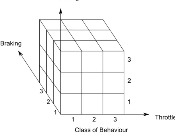
a cycle (Figure 2.3) as the driver is constantly going through this process and the actions taken by the driver have an impact on the situation at hand. The impact of the driver’s actions must then be perceived by the driver in order for another action to be carried out for further progress through the road environment. To form a complete hierarchical model of driver behaviour, the three aforemen-tioned models can be combined to form a 3-dimensional model that completely describes all aspects the driving task (Figure 2.4)[7, 8].

Figure 2.3:The driving process represented as a cycle, [4]

2.3 Motivation and Risk Management

(23)

Figure 2.4:Three dimensional driver model, [7]

outcomes, while other drivers may believe that behaving in such a manner carries too much risk and that the potential positive outcomes do not outweigh the negative ones. The subjective norm is what the general population believes to be acceptable behaviour; if the majority of people behave in a certain manner, a driver may use that information to gauge how they should behave and whether or not the way in which they are behaving would be perceived favourably or unfavourably by the general population. Perception of control describes the driver’s sense of ability to accomplish a task in the driving environment, which is governed by what the driver feels are their own limits as well as the limits of the vehicle.

(24)

case of the Zero Risk Theory, it is proposed that the ultimate goal of the driver is to avoid any and all risk; this is made possible as drivers learn the required actions in order to avoid collisions. What is interesting with regard to the two aforementioned theories is that they are essentially a contradiction of each other, since, according to Wilde, at a state of zero risk nothing is gained or lost and thus no progress is made. In his criticisms of both methods, Vaa established an interesting concept of target feeling [11]. In his opinion, the Risk Homeostasis Theory is too rigid in its assumption of target risk being a number and that the Zero Risk theory fails to establish why drivers will feel safe traveling at a given speed, for example. According to Vaa, the target feeling is achieved by the driver in a given situation where the driver feels comfortable and without risk. In a manner of speaking, he has merged the two theories by taking the aspect that drivers attempt to achieve a target value (in this case a feeling of safety) and as a result,in the driver’s opinion, there is no risk.

The Task-Capability model was proposed by Fuller [9]. The model works based on the fact that drivers have a limited amount of capability and that tasks have a demand associated with them that requires a certain amount of capability. For the majority of driving situations, the driver capa-bility outweighs the task demand; for such situations the driver is able to maintain control of the vehicle. When the task demand exceeds the driver capability, the driver loses control of the vehicle (Figure 2.5). When loss of control occurs, the likelihood of a collision is increased significantly; however, it is possible to avert a collision either through the actions of other drivers or through a so-called "lucky escape". When describing driver capability, there are several aspects for considera-tion. There are physical abilities, such as speed, that affect reaction time, coordination and strength, and mental capabilities, which are determined by the driver’s experiences as well as any training they may have received. To describe the task demand, there are four different categories that affect demand. The first category is the road environment, which encompasses aspects like visibility, road signs and road design (straight, curved etc.); the second category is related to traffic and the other vehicles in the driving environment; the third category is related to characteristics of the vehicle being driven; and the fourth category is the speed and direction of the vehicle. The fourth category is the only one over which the driver has any level of control.

2.4 Behavioural Adaptation

(25)

Figure 2.5:Task-Capability Model, [9]

(26)

2.5 Safety Margins

Safety margins have significant implications for driver behaviour and determining risk, as drivers create a series of imaginary regions around themselves within the driving environment. Drivers establish a safety region around themselves that consists of a risk threshold[15]. Once this threshold is breached the driver has a greater feeling of risk and that a collision may occur. The establishment of these safety margins is generally based on time and space. It has been suggested by Gibson and Crooks that drivers attempt to locate gaps in time and space within the road environment to which they refer to as thefield of safe travel[16]. These gaps are pathways that allow the driver to progress through the road environment without being impeded (Figure 2.6).

Figure 2.6:The field of safe travel as described by Gibson and Crooks, [16]

(27)

there is potential for the field of safe travel to be cut off abruptly to the point of cutting into the min-imum braking distance and inducing the instantaneous application of maxmin-imum braking. In such a scenario a collision is highly probable.

The field of safe travel is defined by the number of different types of boundaries. The first type of boundary is the natural boundary which consists of obstacles along with environmental factors such as lighting (day or night, glare), weather and terrain. Vehicle capability also limits the field of safe travel; while a portion on the inside curve of a road may be unimpeded, it may still be impossible for the vehicle to travel along that path as the tires may not have enough grip to allow such a tight trajectory. While obstacles themselves serve to define the field of safe travel, drivers will typically not follow a path where they come in contact with the obstacle; therefore, the region around the object, known as theclearance regionalso defines the field of safe travel. Moving obstacles have clearance where the vehicle will be closest to; therefore, it may appear that an object is within the field of safe travel as it might be in front of the vehicle in its path. However, once the vehicle arrives at the point, the object will have moved. Such is the case for a pedestrian crossing the street or even a vehicle following another at higher speeds. Potential obstacles have an uncertainty attached to them; such situations occur when the driver may not be able to see part of the road environment ahead of the vehicle, as with blind corners, or when coming over a hill, the assumption is that the path is clear; however, the potential exists for there to be an obstacle. Finally, there are legal obstacles, which consist of things like speed limits or the information from signs such as a stop sign.

2.6 Error Quantification

In order to model driver performance and to determine whether or not a driver’s behaviour can be considered appropriate, any deviation from desired behaviour can be viewed as an error. Driving errors have some relation to safety margins. Any behaviour that takes the driver outside of the established safety margin is likely an error of some nature, since it puts the driver at an increased risk of being involved in a collision. Driving errors can occur at all three levels of driver behaviour and are classified as either being slips/lapses or mistakes[17]. At the knowledge-based performance level of driver behaviour, errors are considered to be mistakes; these errors occur due to incorrect or limited knowledge of the driving situation, which results in the wrong course of action taken by the driver. At the rule-based level, errors are also classified as mistakes; generally these errors are the result of misapplying a certain rule to the given situation. Finally, at the skill-based level, errors are regarded as slips or lapses. Such an error is due to an action carried out by the driver unconsciously in the same manner that all activity at the skill level is carried out–without cognitive thought.

(28)

the use of time related measures. Several methods for time related measures are discussed by van der Horst[8]; he differentiates between methods that can be used for either lateral or longitudinal control. For lateral control of the vehicle, the most heavily discussed measure is the Time-to-Line Crossing, which, as the name suggests, gives the amount of time before a vehicle crosses the line marking a lane and wanders over into another lane. To calculate the Time-to-Line Crossing, the lateral position, heading angle and speed are used. The driver has control over these parameters through the steering angle. For longitudinal control, several measures are proposed which, are Time to Collision (TTC), Time to Intersection (TTI) and the Time to Stop Line (TTS). The Time to Collision measure, indicates the amount of time before two vehicles in the driving environment collide since one is interfering with the path of another; there are several different forms of the Time to Collision measure which describe certain aspects of the event. One form of TTC is TTC braking (TTCbr) which is the time remaining before a collision at the point where the driver begins to apply

the brakes; there is also the minimum TTC (TTCmin) which describes the point in time during the

event where the time before a collision was at its smallest. This measure is particularly useful for describing how close a collision was to occurring. The Time to Intersection (TTI) measures the time needed to reach a major road when approaching it from a minor one. The TTI decreases as the vehicle approaches the intersection and it is affected by deceleration, it is possible to reduce the rate that TTI decreases through gradual deceleration. The Time to Stop Line (TTS) is a similar measure to (TTI); however, rather than referencing an intersection, a specific stop line is specified that may correspond to a certain object in the driving environment is specified.

2.7 Modeling Methods

(29)

in terms of importance are the auditory and tactile channels, with more importance being placed on the tactile channel; however, according to MacAdam, both are useful at providing additional infor-mation with regard to the situation. The list of essential components for a driver model is based on physical attributes and consists of:

• a transport delay time to consider reaction times

• the use of preview to sense lateral and longitudinal control

• adaptation provisions for changing conditions

• a linear regime "crossover model" near what is known as the crossover frequency

• the presence of an internal vehicle model to estimate future responses

There is also a list of secondary components that are not as essential; however, they may serve to further enhance the driver model. The list includes the following components:

• provisions for processing incoming signals to account for neural delays, thresholding, etc.

• neuromuscular filtering elements for output channels such as steering, braking and throttle response,

• previewed path adjustment capabilities to account for skill related abilities or preferences in paths

• the ability to adjust speed according to upcoming lateral path requirements to improve path tracking

• provisions for surprises or unexpected situations

• inclusion of skill factors to account for different skills and experience levels

(30)

regarded as there are inaccuracies that are known to exist in the model. Ultimately, the research by Tustin revealed that modeling human behaviour through the use of mathematical equations is extremely difficult given the amount of variation that exists in human behaviour, especially from person to person.

The Quasi-Linear model is another control theory model that was developed by McRuer and Krendel as discussed by Jürgensohn[19]. In order to model driver behaviour, second-order linear differential equations are used[19]. The model uses five parameters, which are the driver reaction time, the neuromuscular delay, and a gain along with both a lead and lag factor. To create a model us-ing this method, these parameters must be found in a catalogue established by the researchers, which greatly limits the model’s capability. Another model closely related to the Quasi-Linear model that Jürgensohn discuses as well is the Crossover model, which was also developed by McRuer and Krendel. This model is a somewhat simplified form of the Quasi-Linear model that uses an integra-tor and a phase correction for the reaction time and requires two parameters: the reaction time and the crossover frequency. One significant property of this model is that it assumes that the driver and the vehicle are one system; the model is said to often produce a fairly precise description of driver behaviour; however, it too is limited in the same manner as the Quasi-Linear model as it requires either empirical data or parameters from a catalogue.

(31)

terrain is added.

Figure 2.7:Lateral Control Model by Weir and Chao, [20]

(32)

Figure 2.8:Leading vehicle and following vehicle, [21]

(33)

A lateral driver model based on adaptive predictive control was developed by Ungoren and Peng[22]. The basis of the model is to correct the error in the actual position of the vehicle on the road versus the desired one, as seen in Figure 2.10. The lateral position is determined as a function of vehicle state and the steering angle. The proposed model is said to contain three key components of human driving: the use of preview information, off-line adaptation and driving style. For the preview component of the model, selecting the proper preview time is critical since a longer preview window introduces an increase in tracking error; however, the vehicle is said to be more stable. This was found when validating the model and using preview times that were described as being long, medium and short in length. The initial assumption regarding steering angle was that it was fixed throughout the preview window; however, if it is adjusted throughout the preview window it reduces tracking error. Continuous adjustment of steering angle is not a realistic representation of driver behaviour; however, it is likely that some adjustment will occur. Therefore the model often accounts for one adjustment in steering angle during the preview window; this was found to have a similar effect on tracking as shortening the preview window. The model also accounts for driving style, as it was found that drivers control the vehicle based on different cues. For example, experienced drivers use yaw information more than inexperienced drivers. Ultimately, following data analysis from 22 subjects operating a driving simulator, it was found that results from the model correlated well for the most part with the data obtained from the driving simulator.

Figure 2.10:How the model corrects the actual path according to the desired one, [22]

(34)

and lateral control models (Figure 2.11). For processing information, queuing theory is used and in the case of driver models, the driver is represented by a server and the incoming information is represented as clients. The queue temporarily stores these clients until they can be handled by the server. Different types of queues exist, some work simply on a first come first served basis, while some are capable of giving priority to certain clients. In the case of driver modeling, the latter type is best suited. For the driver model, two separate queues are used: one is dedicated to processing visual information, while the other is said to process vestibular information, which consists of motion that is perceived by the sense of balance. The next aspect of the model that is considered is the determination of a reference value, which, in this particular case, is the desired velocity of the vehicle. To determine the desired velocity, a finite state machine (Figure 2.12) that is based on the scenarios encountered in the road environment and consists of seven states numbered 0 through 6 is used. State 0 is the initialisation state when the automat is first called. State 1 (straight line): there is no road curvature within sight and the radius (ρ(t+tf)) is equal to infinity.

State 2 (approaching a curve): the driver can see a curve and may need to adjust the velocity of the vehicle, to calculate the appropriate reference velocity several parameters are used such as the curve radius, the road width and yaw angle. State 3 (braking): at this stage braking is necessary and the necessary amount of braking is determined in order to attain the desired velocity. State 4 (before the curve): at this stage the desired velocity is nearly attained; however, some light braking may still be required. State 5 (curve): the vehicle is now travelling at the desired velocity, minor adjustments may be necessary based on lateral acceleration and what the driver feels. State 6 (accelerating): the final state where the driver begins to accelerate, this may occur slightly before the curve ends. The final portion of the model is the controller itself. As with many models two separate systems are used for longitudinal and lateral control with both using a General Predictive Controller. For the longitudinal controller, the inputs are the desired and actual acceleration while the outputs are the throttle angle and the brake pedal force. To determine the appropriate amount of engine or braking torque required, the controller uses maps that contain both engine and brake torque with respect to both desired acceleration as well as vehicle velocity. While the braking portion of the controller is very similar to the accelerating portion, it also adds the ability to consider the effect of engine braking. The operating principle used for the lateral controller is to minimize the offset of the vehicle to an ideal line on the road, the output of this controller is the steering angle and the offset is measured from the centre point of the front axle.

(35)

driver-Figure 2.11:Model structure proposed by Kiencke and Nielsen, [23]

(36)

vehicle-environment (DVE) simulation system[24]. To model the driver handling behaviour in the DVE both mental behaviour and physical action are considered. In their study, three different ma-noeuvres were considered: a single line motion which is typically used in a lane change, a double line motion as seen in the overtaking of another vehicle and sine line motion which is used while negotiating an s-curve turn. The inputs to the neural network that are used in this model are the yaw rate, lateral velocity, lateral acceleration, roll angle, roll angle velocity, lateral displacement and preview lateral offset. The outputs of the system consist of the steering wheel angle as well as the steering wheel angle velocity. Figure 2.13 presents the general architecture for feedforward neural network structures.

(37)

Figure 2.13:General feedforward neural network architecture, [25]

2.8 Potential Applications for Driver Models

Up to this point, most of the research into driver modeling has been for the purpose of developing driver assistance systems or driver information systems. The models are used to study both the effects of implementing these devices on driver behaviour as well as to design them to be more ef-fective. There exists several other applications for the use of driver models, one area in particular is the optimization of drive cycles in hybrid vehicles. Hybrid vehicles utilize two methods of propul-sion and as a result energy management is a significant issue in their development; driver modeling can aid in optimizing fuel economy and maintaining proper charge sustenance. To achieve this goal, a control device will determine the appropriate torque distribution. Also some systems may actually work with the driver to either alert them or assume control in order to operate in a manner that increases fuel efficiency.

(38)

The application of driver modeling for accident reconstruction has been undertaken by Jurecki & Stanczyk[27]. In their work they state that there are many factors that contribute to accidents thus making it difficult to determine the exact cause. In their opinion accident reconstruction is the next logical step for the application of driver modeling, following their use for vehicle development and then vehicle control systems development. The authors focus on the concept of risk time, which is a function of both vehicle speed and the distance to an obstacle and describes how much time a driver has to react to a scenario. A relationship between reaction time and risk time was discovered with reaction times increasing with risk time. This relationship is to be expected as drivers will have more time to react and they will be slower to do so, as seen in Figure 2.14. To characterise driver behaviour in pre-accident situations, braking and steering manoeuvres were evaluated along with risk time; by using this data in conjunction with a driver model previously developed by the authors, it is believed possible to reconstruct an accident and determine the cause, since there is now more insight on how drivers will behave when presented with an accident scenario.

Figure 2.14:General relationship between reaction time and risk time, [27]

(39)

(40)

Theory

3.1 Artificial Neural Networks

3.1.1 General Information

While there are many possible methods to create a driver model, as described in the previous chapter, for this particular project Artificial Neural Networks were chosen. Although it is unknown if this is necessarily the best method to create a driver model, part of the goal of this research is to discover whether or not this is the case. The principle behind Neural Networks is to mimic the function of the human brain; they are capable of learning the behaviour of a certain phenomenon based on provided information. Neural Networks are capable of representing a broad range of systems but there is one major distinction in that they can be used for either function approximation or data organization. Typically the systems that are modeled using neural networks fall into one of the two aforementioned categories.

In order to develop a neural network, it must first be trained; this is done by presenting a dataset that contains both input and desired output, or target variables. The goal of training is to allow the network to be exposed to the input variables that stimulate the system along with their corresponding response; using this information the network is able to learn how the system will behave under the conditions characterized by the presented training dataset. This type of training is known as supervised training. Unsupervised training is another form of neural network training and it is typically used in clustering and pattern recognition applications. The idea behind unsupervised training is for the network to group like variables together when presented a dataset. It does this by assuming that inputs within a certain region of the input space are similar and thus represent a similar behaviour or characteristic. An important point to note is that neural networks are very effective at making generalizations and very effective at interpolating; however, it is widely accepted

(41)

that neural networks are not particularly strong at extrapolating data [28]; therefore, when selecting a dataset it is important to ensure that the number of data points is sufficient to span as large an area as possible (or practical) such that the network is trained for the widest number of possible scenarios.

Artificial Neural Networks are structured very much like their biological counterparts; they contain elements known as neurons (Figures 3.1 & 3.2) which are connected to one another as well as to data. The network may contain multiple layers of neurons; however, there is a minimum of three layers: The input layer, which, like the name suggests contains the input data. The next layer is the hidden layer (or layers as often more than one may be utilized). This is where much of the generalization is performed. The final portion is the output layer where the network gives the output representing the response of the system. The hidden layers and the output layer are comprised of a series of neurons. In the case of the output layer the number is defined by the number of output variables; however, for the hidden layer the number is somewhat arbitrary. The goal is to achieve a desired level of accuracy with a minimal number of neurons.

Figure 3.1:Structure of a feedforward neural network, Adapted from: [25]

(42)

of weights, a bias and a transfer function. The role of the weight is to connect network inputs to the neuron or to connect the output of one layer of neurons as inputs to another. The number of weights in each neuron corresponds to the number of inputs to that particular neuron, in the case of a single hidden layer network, a hidden layer neuron will have the same number of weights as network inputs while an output layer neuron will have the same number of weights as there are hidden layer neurons. Each weight is multiplied by its corresponding input and all of the products are summed together. The role of the bias is very similar to that of the weight; however, each neuron only contains one and in some cases a bias may not be used at all. Essentially a bias is weight that acts on an input equal to unity in the same way that a weight acts on an input from the dataset. It acts to shift the sum of the weighted inputs by the bias value. The final component of neuron is the transfer function which may also be referred to as an activation function. A variety of functions can be used as the transfer function in the neuron, the most important distinction being between linear and non-linear transfer functions. In the case of hidden layer neurons, the transfer function used is generally non-linear with the most common being either the logistic function (Figure 3.3 & Equation 3.1)[29] or the hyperbolic tangent function (Figure 3.4 & Equation 3.2)[29]. In the output layer typically a simple linear activation function is used.

Figure 3.2:Structure of a single neuron, [28]

(43)

[ht pb]f(t) = 1

1+e−t (3.1)

Figure 3.4:Plot of Hyperbolic Tangent Function, [28]

[ht pb]f(t) =1+e

−t

1−e−t (3.2)

Having defined all the critical elements of the neuron it is now possible to describe how they all work together to approximate the behaviour of a particular system. First, each input will be passed to each hidden layer neuron where, as mentioned before, they will be multiplied by the corresponding weight. The next step is to sum the products of all the inputs multiplied by the weights and to add the bias. Each summation is then passed through the transfer function at, which point they become the outputs of the neurons. The same procedure is repeated through the next hidden layer or the output layer depending on the overall network structure. Updating the weights is the method by which the network learns to model the system. As an initial starting point an arbitrary set of weights is chosen and the data is passed through the network. The output of the network is then compared with the target output of the system and the error between the two outputs is calculated and then used to update the weights using one of many available training algorithms which will be discussed in greater detail in the following section. Please note that the aforementioned process is specific to supervised learning.

3.1.2 Training Algorithms

(44)

through the neural network to update the weights until a satisfactory minimum error is achieved. Several variants of gradient descent methods exist which will be discussed later in this section. In the case of second order methods, the second derivative of the error surface with respect to the weights is used to determine the curvature of said surface, which is used to update the weights. Second order methods are more powerful and have a tendency of training faster; however, they do require more computing resources. It is also important to mention that there are several ways of calculating the error; a commonly used method is the mean squared error or MSE (Equation 3.3)[29].

E= 1

2N N

∑

i=1

(zi−ti)2 (3.3)

where,

E=the error

N=the size of the training set

z=the network output

t=is the target output

The simplest form of neural network training is backpropagation learning. As the name implies the error associated with the neural networks for a given set of weights is used to update the weights for the next iteration. The formula for updating the weights using backpropagation training is given in (Equation 3.4)[29]. Essentially the direction of steepest descent is determined by noting that it is in the opposite direction of the previously calculated gradient, dm[29]. The gradient is then

multiplied by a pre-determined factor called a learning rate, ε, and it is then added to the current

weight. The only parameter that the analyst controls is the learning rate which is essentially opti-mized through trial and error, ranging between 0 and 1. The ideal learning rate is able to quickly and efficiently determine the minimum error yet still descend the error surface in a smooth manner to the global minimum. If the error rate is too small it may take a long time to attain convergence and if it is too large it may oscillate around a solution yet never reach the minimum point. A param-eter known as momentum is an additional term that can be added to the backpropagation algorithm (Equation 3.5[29]). Once again the parameter ranges between 0 and 1 and its purpose is to consider previous weight changes in order to dampen potential oscillations.

wm+1=wm+∆wm

∆wm=−εdm

(45)

(46)

where,

w=the weight

ε=the learning rate

dm=the derivative or gradient.

∆wm=µ∆wm−1−(1−µ)εdmw (3.5)

where,

µ=the momentum term

Another commonly used set of first order training algorithms uses conjugate vectors to locate the minimum error. They are commonly referred to as conjugate gradient methods. Conjugate gradient methods differ from steepest descent methods in that descent of the error surface follows the direction of a vector that is conjugate to the steepest descent vector. In simple terms a conjugate vector is orthogonal to the steepest descent vector; see Equation 3.6 for the definition of conjugate. The advantage of conjugate gradient algorithms (Equation 3.7) is that they are supposedly capable of obtaining second order information without the need to actually calculate the second derivative. Unfortunately some of this information may be lost through a procedure called restarting where after a certain number of iterations, the solution restarts following the direction of steepest descent. Restarting must be employed to increase the rate of convergence, otherwise it is only linear[30]. There are several theories on how often the algorithm must be restarted. A discussion of such methods is beyond the scope of this thesis; further reading is available in other publications, [30, 31, 32]. The main difference between the variants of conjugate gradient methods is the manner in whichβkin Equation 3.7 is calculated, the method shown is just one example.

pt_iGpj=0 wheni6= j (3.6)

where,

G= an arbitrary matrix

(47)

w_k+₁=wk+αkpk

pk+1=−gk+1+βkpk

βk= yt_kg_k+₁

yt_kpk yk=gk+1−gk

(3.7)

where,

w=the weight

g=the gradient.

p=the search direction

α=appears to be the learning rate however this is not explicitly stated k=kthiteration

(48)

Hessian matrix thus allowing it to run using fewer system resources. H=        

∂2E

∂w2_i

∂2E

∂wi∂wj · · ·

∂2E

∂wj∂wi . ..

.. .

∂2E

∂wm∂wn

        (3.8)

∆wm=−εdm ds

m

(3.9)

where,

wm=the weight

ε=the learning rate

dm=the 1st derivative of the error surface

d_ms =the 2nd derivative of the error surface

∆wm=− dm ds

m+eλ

(3.10)

where,

eλ₌_{the conditioning term}

3.1.3 Types of Neural Networks

Until now, the discussion regarding neural networks has focused mainly on the multilayer percep-tron or MLP, which is the most basic form of neural network; however, many different types exist with each being suitable for a different purpose. As briefly mentioned earlier in the preceding sec-tions, there are clustering networks which are used to organize data. The way in which they work is that they will take a dataset and look for certain trends in the data. Based on these trends the data will then be grouped into various clusters in which the data exhibits similar characteristics. Such architectures are often used for pattern recognition problems in order to classify information of some sort. Examples of fields that use them are the medical field and image processing.

(49)

the same state is used instead (Figure 3.7). The latter architecture is said to be more accurate and based on the author’s experience, it appears to train significantly faster.

Figure 3.6:Closed loop NARX network, [28]

Figure 3.7:Open loop NARX network, [28]

(50)

network, the spread is the only parameter that the analyst can tune to optimize it. Another important point to note is that there exists what is called an exact RBFN where the size of the network is dictated by the size of the training set, such that there is a neuron for each data point in the input set whose center is equal to that particular input. The main drawback is that the network becomes very large, perhaps too large and inefficient. An alternative to this approach is start with one neuron and train the network by continuously adding a neuron and updating the weights until a network deemed acceptable according to the standards set forth by the analyst is created.

Figure 3.8:Plot of Radial Basis Function, [28]

f(x) =e−|x−w|b (3.11) where,

x=the network input

w=the weight or neuron center in the input space

b=the spread

3.2 Vehicle Dynamics

While the focus of this thesis is not on vehicle dynamics, it is the opinion of the author that it is important to discuss some elementary vehicle dynamics properties given the influence they have on vehicle handling, which ultimately influences the driver’s decisions. Most of the decisions that a driver will make are either based on visual information (what the driver sees) and vestibular in-formation (what the driver feels). Other properties are used as well; however, these are the two principal ones.

(51)

related to the behaviour of the tire and the property known as slip. In the longitudinal sense it is known as the slip ratio and in the lateral sense it is known as the slip angle. Until a certain degree of slip the tire will behave in a linear fashion; however, beyond that point the behaviour becomes nonlinear and therefore more difficult to predict[35]. As a result, the average driver is restricted to the linear regime and the car is much more predictable. Typically, if an average driver enters the non-linear range of operation, the result is often dangerous as they typically reach the grip limit of the tires. It is only highly trained and skilled drivers that are capable of operating in this range. The data used in this study likely falls within the linear regime.

Another important aspect of vehicle dynamics is handling and the vehicle’s steering tendencies. Vehicles can handle in three different manners; they will either understeer, oversteer or experience neutral steering. In the case of understeer, the vehicle will have a tendency of taking a corner with a wider turning radius if the speed is increased[35]. During oversteer the turn radius will decrease with speed, and neutral steer occurs when the vehicle keeps the same radius. Ideally neutral steering is desirable; however most vehicles are designed to have some degree of understeer. The reason for this is that understeer is a stable state such that if the driver were taking a curve too fast they would simply need to reduce their speed in order to safely negotiate it. In the case of an oversteering vehicle, it can become very unstable before the driver can safely realize it; therefore, such vehicles are prone to losing control and spinning suddenly. Once again, there are some applications where highly skilled drivers may prefer some degree of oversteer; however, its use in everyday applications is highly unrecommended and potentially dangerous. There are several factors that influence the handling characteristics of a vehicle: the first being weight distribution and the location of the center of mass, the next being the lateral force being developed by the tires which, in turn, is influenced by the properties of the tires themselves as well as by the stiffness of the suspension.

(52)

(53)

Training Data

In order to develop a neural network, a set of training data must be acquired such that the network can learn the behaviour of the system, as mentioned in Chapter 3. To develop a driver model, the training data must consider three key elements, which are the driver, the vehicle and the road environment. It is important to recognize that for the purpose of this research the driver is nothing more than a controller, albeit a very sophisticated controller. As a result there will be both a set of input data as well as a set of output data. Drivers will use information of the vehicle’s behaviour and information from the road environment to make their decisions on the vehicle control inputs to use. This information will constitute the input variables, while the driver’s actions will be the output variables.

In order to obtain driving data, there are two methods available. The first is to instrument a vehicle and ask a selected group of people to act as test subjects and to drive a specified route in the vehicle. While this occurs their actions, along with the vehicle behaviour are recorded. The other method is to set up a driving simulator on a computer. The former method has the advantage of being more accurate since all of the factors in terms of the vehicle’s performance and roadway information can be considered. The drawback to this method is that a lot more resources are required, which can increase the cost as well as the time needed to acquire the data. The latter method using a simulator is much easier and much cheaper to use, since the subjects can perform the test in an office environment and fewer resources are required. The issues with using a driving simulator are concerns with accuracy. Constructing a simulator that can accurately model the behaviour and response of a vehicle can be very difficult and costly. As an example, when driving a vehicle on the road it is likely to behave differently than in a simulator due to non-linearities and the behaviour of the components’ materials, particularly in the case of the tires. The question of accuracy also calls into question the overall validity of any test administered on a driving simulator.

(54)

4.1 Driving Simulator

To acquire data, the Groupe de Recherche en Analyse du Mouvement et Ergonomie (GRAME, translated: Movement and Ergonomics Analysis Research Group) at l’Université Laval in Québec City, PQ; was contacted as they possess a driving simulator and have substantial experience running simulations, particularly for elderly drivers. The simulator is developed by Systems Technology Inc.(STI®), it is referred to as STISIM and it operates their Drive 2.0 software[36]. STI® offers a variety of simulator configurations both in terms of hardware and software; descriptions of the different types of simulators are listed in [37]. The arrangements offered range from very simple setups that are relatively inexpensive and can be used with a desktop computer and controls used for gaming to sophisticated cab style simulators with projectors that provide steering feedback to the driver. The simulator installed at Laval shown in Figure 4.1 is an open cab simulator; however, it does not offer any steering feedback to the driver. The simulator uses an image approximately 1.45m high and 2.0m wide projected onto a flat wall situated approximately 2.2m away from the simulator. The field of view generated by the projector is 40 degrees horizontally and 30 degrees vertically. The simulator is also equipped with a video camera to record the driver’s actions[36]. All of the driving simulator interfaces are instrumented such that all of the steering wheel, throttle pedal and brake pedal movements are recorded. The simulator can record 50 data channels[38]; however, only a select number of the channels are used for model development. Ultimately, the channels of interest for this project are the longitudinal velocity and acceleration, Vx and Ax, respectively,

the lateral position, velocity and acceleration, Y, Vy and Ay, respectively, speed limit, Vlim and

road curvature,ρ. These seven channels will act as the input variables for the neural network. The steering wheel angle,θ, throttle pedal, Tpinput and brake pedal input, Bp, will act as target variables

for the network as they will be the output from the network once it is simulated.

In terms of software, the vehicle model is based on a simulation tool developed for the NHTSA known as Vehicle Dynamics Analysis NonLinear (VDANL)[37]. As the name suggests, the model provides a non-linear analysis of the vehicle performance, and it includes a sophisticated tire model referred to as STIREMODEL. The motivation, according to STI®, for using a high fidelity vehicle dynamics model is "to achieve realistic feel and motion cueing and to be able to provide hardware-in-the-loop interaction with elements such as steering and braking"[37]. STI® does acknowledge that some of the computer analysis components of the model have been disabled in order for the model to be able to run in real time, they refer to the modified model as VDANL/RT, this variation also has an additional input-output component added to it. The software used in the simulator at Laval is a simplified model that is linear and according to STI® _{"has no notion of individual}

(55)

no throttle inout and 1 is full throttle input, and braking is typically measured either using the force required to move the pedal or the brake master cylinder pressure. Instead, the linear model considers the accelerations due to throttle and braking; it does, however, keep a record of the raw inputs. This does create some complications for the development of the model that will be discussed in Section 4.3. Another complication that arises from the use of the simplified model is that because there is no notion of individual wheels, there is no steering ratio between the angle of the steering wheel and angle of the steered wheels at the road. The lack of a steering ratio is problematic when validating using a vehicle simulation program such as CarSim® as it uses the angle at which the wheels are being steered while the data from the simulator is the angle of the steering wheel; without a steering ratio there is no way of relating these two parameters. Ultimately the simplified linear model may be a satisfactory and more cost effective solution for the purposes that it is being used for by GRAME in terms of giving an estimate of driver performance from the standpoint of observing physical abilities. A non-linear model would provide a more realistic model and allow for the creation of a more accurate representation of the driver’s behaviour, particularly when constructing the model using a neural network. Such a model would be more costly; however, future work should endeavor towards using a non-linear model. Further discussion regarding this idea will be made in the conclusions and recommendations chapter.

(56)

The data that is used in the neural network is distance-dependent as opposed to time dependent. This approach is taken because the subjects completed the driving scenario at different rates. Basing data extraction on time is not appropriate as the proper events will not be recorded; however, because the scenario is the same for all subjects, extracting the data based on the distance traveled will provide the desired events. The sample rate of the simulator is constant at 30 Hz., therefore the datasets will all be of different sizes for different subjects depending on the amount of time taken by the subject to complete the scenario. In this discussion, scenario describes the entire course that the subject is asked to follow. It is important to note that while it is not explicitly recorded, time is considered in the input dataset as each segment is a timeseries concatenated to form one large dataset. Training the neural network requires presenting it with the expected outcome for a given series inputs. Based on that expected outcome a generalization is made, therefore, the time at which each event occurs is ultimately irrelevant.

4.2 Data Acquisition

(57)

4.3 Data Processing

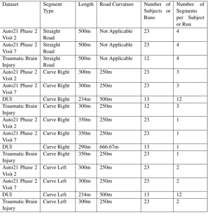
Once the data was acquired from the simulator extensive processing was required to prepare it to train the designed neural network. As discussed previously, there were many data channels recorded from the simulator; however, only a select few were required to construct the model. As also previously noted, segmentation of the data was required such that what was occurring in the road scenario was known and that it could be associated with the appropriate subject or test run. As mentioned, there were four datasets that were used in training the neural network. In terms of the scenario, it was the same one used for the the two visits studying elderly drivers and for the study that focused on the retraining following a traumatic brain injury. A comprehensive breakdown of the driving scenarios is given in Table 4.1.

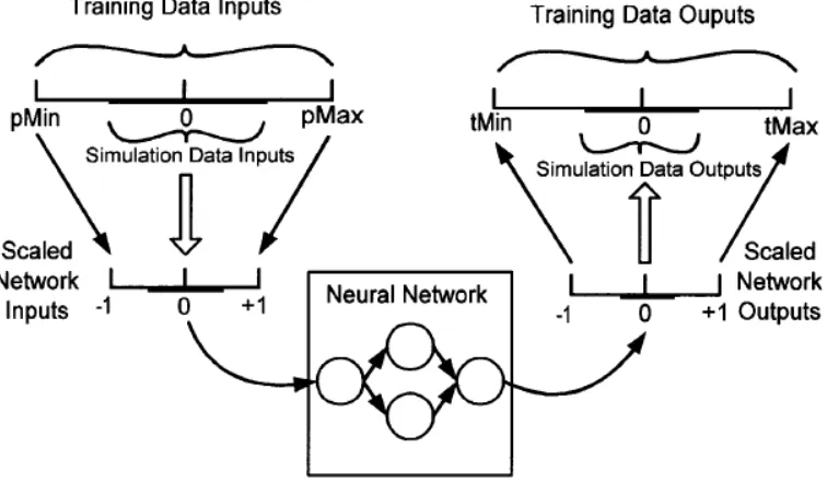
In order to obtain the data in a useful form, a script was written in MATLAB® that would extract the desired variables for each segment. The manner in which the script functions is that the distance corresponding to the beginning of the segment is presented; the script then searches through the distance variable until it finds the first value equal to or greater than the presented value. It then identifies the "handle" of that variable and uses it to find the appropriate value for each of the variables that are to be extracted (The handle is an identifier of a variable assigned by MATLAB®, it is associated with the index of a matrix)[40]. This same process is repeated to find the end of the segment; once these two values are found they are used to set up a loop that extracts all of the desired data in between these two points. Once all of the data was extracted, it was then concatenated into one data file containing in excess of 380,000 data points. Following the concatenation, the data was then normalized between -1 and 1; this is common practice when conditioning data for use in neural networks; the process is illustrated in Figure 4.2 .