Adaptive Channel Estimation for Turbo Decoding

(1)

University of Windsor University of Windsor

Scholarship at UWindsor

Electronic Theses and Dissertations Theses, Dissertations, and Major Papers

2012

Adaptive Channel Estimation for Turbo Decoding

YU QING GUO

University of Windsor

Follow this and additional works at: https://scholar.uwindsor.ca/etd

Recommended Citation Recommended Citation

GUO, YU QING, "Adaptive Channel Estimation for Turbo Decoding" (2012). Electronic Theses and Dissertations. 127.

https://scholar.uwindsor.ca/etd/127

(2)

Adaptive Channel Estimation for Turbo Decoding

by

Yuqing Guo

A Thesis

Submitted to the Faculty of Graduate Studies through Electrical and Computer Engineering in Partial Fulfillment of the Requirements for the Degree of Master of Applied Science at the

University of Windsor

Windsor, Ontario, Canada

2012

(3)

Adaptive Channel Estimation for Turbo Decoding

by

Yuqing Guo

APPROVED BY:

______________________________________________ Dr. Luis Rueda

School of Computer Science

______________________________________________ Dr. Huapeng Wu

Department of Electrical and Computer Engineering

______________________________________________ Dr. Behnam Shahrrava, Advisor

______________________________________________ Dr. Chunhong Chen, Chair of Defense

(4)

iii

DECLARATION OF ORIGINALITY

I hereby certify that I am the sole author of this thesis and that no part of this

thesis has been published or submitted for publication.

I certify that, to the best of my knowledge, my thesis does not infringe upon

anyone’s copyright nor violate any proprietary rights and that any ideas, techniques,

quotations, or any other material from the work of other people included in my thesis,

published or otherwise, are fully acknowledged in accordance with the standard

referencing practices. Furthermore, to the extent that I have included copyrighted

material that surpasses the bounds of fair dealing within the meaning of the Canada

Copyright Act, I certify that I have obtained a written permission from the copyright

owner(s) to include such material(s) in my thesis and have included copies of such

copyright clearances to my appendix.

I declare that this is a true copy of my thesis, including any final revisions, as

approved by my thesis committee and the Graduate Studies office, and that this thesis has

(5)

ABSTRACT

A new adaptive filter is proposed for the turbo decoding on Rayleigh fading

channels with noisy channel estimates. The turbo decoder that is used over Rayleigh

fading channels is exactly the same as the one used on Additive White Gaussian Noise

(AWGN) channel. The turbo decoder works very well on AWGN channel [1]-[2], but not

as well on Rayleigh fading channels at that time. In [5], the author assumes there already

exists a fading channel estimator with some estimation errors and develops a new channel

reliability factor and new decision variables for turbo decoding on Rayleigh fading

channels. Hence, Frenger, the author of [5] improved the performance of turbo decoding

over Rayleigh fading channels. Since then, most research has focused on the channel

estimation to reduce the error variances of estimating. However, the extrinsic information

generated from the turbo decoder has some priority information about the transmitted

data bits, which can help us better understand the channel characters. In this thesis, by

using the soft extrinsic information after each iteration of decoding, we re-estimate the

channel and the minimum mean square error (m.m.s.e.) and further update the channel

reliability factor and decision variables at each iteration. Simulations show that signal to

noise (SNR) gain is improved by up to about 1dB at bit error probability of 4

(6)

v

ACKNOWLEDGEMENTS

I would like to thank all of those who made this research possible: especially my

advisor, Dr. Behnam Shahrrava, for his kindness guidance and advice at every step of this

research. I would also like to thank the committee members, Dr. Luis Rueda and Dr.

Huapeng Wu, for their comments and encouragement. I would also like to thank my wife

(7)

TABLE OF CONTENTS

DECLARATION OF ORIGINALITY ... iii

ABSTRACT... iv

ACKNOWLEDGEMENTS...v

LIST OF FIGURES ... viii

CHAPTER I. INTRODUCTION 1.1 Review of the literature ...1

1.2 A new adaptive algorithm for turbo decoding ...3

1.3 Organization of the thesis ...4

II. CHANNEL MODELS 2.1 Basic elements of digital communication systems ...5

2.2 Channel models ...6

2.2.1 AWGN channel ...6

2.2.2 Rayleigh fading channel ...7

III. TURBO CODES AND DECODING 3.1 Turbo encoder ...9

3.2 Maximum a posteriori (MAP) algorithm over AWGN channel ..10

3.3 Turbo decoding over AWGN channel ...13

3.4 Turbo decoding over the Rayleigh fading channel...18

IV. ADAPTIVE TURBO DECODER 4.1 Block diagram of the proposed adaptive filter ...21

4.2 Estimation theory review ...23

4.3 The proposed estimator (2) of channel a ...25

4.4 Implementation of the proposed adaptive filter...28

4.5 The boundary of estimation error variance of the estimator (2) ...30

4.6 Decoding method comparison ...31

V. SIMULATION RESULTS 5.1 General settings ...33

5.2 BER performances with different settings...33

(8)

vii

VI. CONCLUSIONS AND RECOMMENDATIONS

6.1 Summary of contributions ...39 6.2 Recommendations for future studies ...40

APPENDICES

Matlab scripts of the turbo decoder with adaptive filter...42

REFERENCES ...61

(9)

LIST OF FIGURES

FIGURE 1 BLOCK DIAGRAM OF A DIGITAL COMMUNICATION SYSTEM... 5

FIGURE 2 AWGN CHANNEL MODEL... 7

FIGURE 3FADING CHANNEL MODEL... 8

FIGURE 4TURBO ENCODER... 9

FIGURE 5RSC ENCODER... 10

FIGURE 6TURBO DECODER... 16

FIGURE 7BLOCK DIAGRAM OF ADAPTIVE FILTER... 22

FIGURE 8IMPLEMENTATION OF THE ADAPTIVE FILTER... 28

FIGURE 9BER PERFORMANCE WHEN USING ADAPTIVE FILTER (SOLID) VS THE RESULTS OF FRENGER’S (DASHED) ... 34

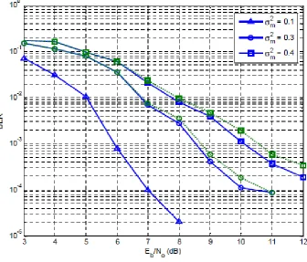
FIGURE 10BER OF THE ADAPTIVE FILTER (SOLID) VS THE RESULTS OF FRENGER'S (DASHED) WITH DIFFERENT σ2_m _{... 35}

FIGURE 11BER WITHOUT SELECTING CRITERIA... 36

FIGURE 12STEP SIZE VERSUS ITERATIONS... 37

(10)

1 CHAPTER I

INTRODUCTION

1.1 Review of the literature

Turbo codes, introduced in [1], have been proven to perform remarkably well on

additive white Gaussian noise (AWGN) channels [1], [2]. The performance of the turbo

codes on Rayleigh fading channels has also been studied since then [3] - [6]. In [6], the

author, Frenger, gave out the exact decoding metric for binary phase-shift keying (BPSK)

signalling on Rayleigh fading channels by assuming that there is a channel estimator

prior to the turbo decoder to provide us with an unbiased channel estimate with a certain

error variance. The conventional turbo decoding metric on AWGN channels needs the

estimation of signal to noise ratio (SNR) [7]. The exact turbo decoding metric over

Rayleigh fading channels needs both SNR and the channel fading factors [3], [8].

However, the channel parameters are assumed to be known by Frenger in [6]. Since then,

many researches have focused on the estimation of channel parameters and the

degradation caused by errors in these parameters, while there is not much research

directly working on the results of Frenger in [5] and [6]. This could be seen from the

number of citations in IEEE: [5] is only cited twice [9], while [6] is cited thirteen times so

far [10], [12].

The effect of SNR mismatch on the performance of the turbo decoding has been

studied in several works. Some research has been proposed for integrating the estimation

process into the turbo decoder over fading channels [9], [11]. In [9], a modified version

of Wiener filtering with initial pilot symbols is proposed, and the bit error rate (BER)

(11)

filtering algorithm with initial pilot symbols. In [10], the exact turbo decoding metric is

simplified. The BER performance is between that of the conventional decoding metric

and the exact decoding metric, but is very close to the BER performance of the exact

decoding metric. In [11], an in-service estimation of the channel reliability factor is

proposed, which uses the statistical computations of the block observations to get BER

performance similar to the exact decoding metric in [6]. In [13], they do not use the fixed

iterations with the turbo decoder, while they do use adaptive iterations for speeding up

the decoding process by aiming at a fixed BER. Once the aimed BER, say10−4, is reached, no further iterations for the turbo decoder are needed. All these estimation schemes can

be seen as pilot symbol aided modulation (PSAM) or as blind channel estimation

methods. Most of these estimation methods ignore the feedback from the turbo decoder.

However, the extrinsic information generated during turbo decoding process has some

priori information about the transmitted data bits, which can help us refine the channel

fading factors.

In [12], a novel idea has been proposed for integrating the extrinsic information

from the turbo decoder to re-estimate the fading channel. However, a mistake is made

during the mathematical derivation approach. There is no relation between the re-estimate

of the fading channel and the extrinsic information as expected. So an incorrect method is

used to make such a connection, which is to approximate the new channel estimate and

its error variance by taking their expected value on coded input data bits .There is no

(12)

3 1.2 A new adaptive algorithm for turbo decoding

In this thesis, based on the results in [6] and [12], we propose a new adaptive

channel estimation algorithm for turbo decoding on Rayleigh fading channels. The

mistake in [12] is corrected. However, the experiment does not go positively as expected

after the correction. The results of the experiment show that the extrinsic information

generated during the decoding process is not totally reliable. The extrinsic information of

some bits is helpful to the channel re-estimation, while the others are not. Future

researchers should pay attention to this point, avoiding unnecessary repeated experiments.

The adaptive decoding metric proposed by this thesis has successfully overcome this

problem by utilizing an effective stop-and-go strategy at the implementation stage as a

selecting criterion. In addition to that, the steep-decent algorithm of Newton’s method is

used to co-operate with the iterative nature of the turbo decoder. The varying step size is

also adopted to achieve faster convergence.

The observations received by the turbo decoder have two parts: the systematic

portion and parity portion. The proposed adaptive filter takes only the systematic

observations and the soft extrinsic information, which is the feedback from the turbo

decoder, as its inputs. This is one of the unique choices of this thesis. Some research

takes the hard decision as the input of the adaptive channel filter for only the amplitude

estimation [14], while some takes only the soft information as the input of the adaptive

filter for SNR estimation [13]. None of them split up the observations into two parts. The

conventional decoding algorithm that is used for AWGN channels is unchanged in this

thesis. However, the exact decoding metric that is derived by Frenger in [6] is updated

(13)

The proposed adaptive filter works better when the block size of the information

gets smaller or the estimation errors of the channel estimator in [6] get bigger. The gain

of using the proposed adaptive filter is about 1dB at the bit error probability of 4

3.5 10× − with some settings. This gain is obtained with minimally increased complexity.

1.3 Organization of the thesis

The organization of this thesis is as follows: In Chapter 2, the basic elements of a

digital system and the channel models are introduced. In Chapter 3, the turbo encoder and

turbo decoding algorithm are reviewed. In Chapter 4, we propose an adaptive filter that

uses the soft information to update the exact turbo decoding metric iteratively over

Rayleigh fading channels. In Chapter 5, simulation results are presented. Finally,

conclusions and future research directions are given in Chapter 6. The whole Matlab

scripts of the proposed adaptive filter and the turbo encoder and decoder are presented at

(14)

5 CHAPTER II

CHANNEL MODELS

To design a channel estimator and analyze the performance of turbo decoding

algorithms, we need to understand the channels that the transmitted data experiences. The

concept of the basic digital communication systems and two channel models are needed

to discuss our contributions

2.1 Basic elements of digital communication systems

The demand for efficient and reliable digital communication systems has rapidly

increased in recent years. It is necessary to minimize bit error probability at the receiver

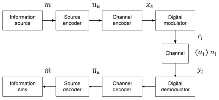
end for higher quality communication. A block diagram of a digital communication

system is shown in Figure 1 [15].

Figure 1 Block diagram of a digital communication system

The information source usually contains redundancy. The source encoder removes

the redundancy of the information to achieve efficiency. The source encoder changes

source information to information sequences. Then the channel encoder adds redundancy

to the information sequences in a controlled way to increase communication reliability.

(15)

is suitable for a physical channel. The transmitted bits will be distorted randomly both in

amplitude and phase due to many factors, such as reflection, refraction, multipath…

At the receiver end, the digital demodulator produces an estimation of the

transmitted data. The channel decoder uses the redundancy and knowledge of the channel

code to detect and correct errors. Finally the source decoder reconstructs the original

information by using knowledge of the source encoding method.

In this thesis, the main concern is channel decoding for binary phase shift keying

(BPSK) signalling over the Rayleigh fading channel.

2.2 Channel models

For better understanding of decoding strategies over the Rayleigh fading channel,

we first need to introduce the additive white Gaussian noise (AWGN) channel model, and

then the fading channel model.

2.2.1 AWGN channel

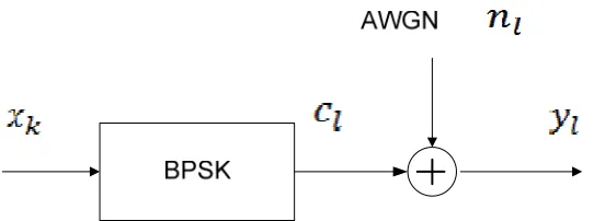
The AWGN channel model, together with BPSK modulator, is shown in Figure 2.

Where xk∈

( )

0,1 are coded data bits. The coded data (systematic bits and parity bits) are inputs to a BPSK modulator, which generates the transmitted channel symbols

(

,

)

l s s

c ∈ − E E . In an AWGN channel, Gaussian distributed random noise, n , with _l zero mean is added to the transmitted symbols. The variance of n is: _l

[ ]

2 0

2

l n

N

(16)

7

Figure 2 AWGN channel model

The signal to noise ratio (SNR) is:

2

0 2

b s

n

E E

N =r× σ (2.2)

where E_b is the energy per information bit, E_s is the energy per actual transmitted

symbol, r is the coding rate, and we have the relationship between the energies and the

code rate,

s b

E r

E = (2.3)

At the receiver end, we have,

l l l

y = +c n (2.4)

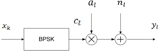
2.2.2 Rayleigh fading channel

The Rayleigh fading channel is a statistic model mostly used by wireless system.

The Rayleigh fading channel with independent additive white Gaussian noise and a

BPSK modulator is shown in Figure 3. Each of the channel symbols, cl, is transmitted on

such model. At the receiver end, we have [16],

l l l l

(17)

where the noise n and the channel coefficient l a are complex valued, Gaussian l

distributed random variables with zero mean that are independent of each other.

Figure 3 Fading channel model

The variances of a and l n are l

2 2

[| | ] 2 ,

[| | ] 2

l a

l n

E a

E n

σ σ

=

= (2.6)

At the receiver we need to know both the amplitude and phase distortion. Such

analysis is more complex than the analysis of the AWGN channel model. We can express

the complex valued channel coefficient a as follows, _l

l

j l lr li l

a =a + ja =r eθ (2.7)

The amplitude and phase probability density function (pdf) of the channel

coefficient a is [17]: l

2 2

( )

1

( ) 0, 2

2 l

a

r l l

a

l

r

f r e

f

σ

θ π

π

−

=

= [ ]

(2.8)

(18)

9 CHAPTER III

TURBO CODES AND DECODING

Turbo codes with maximum a posteriori (MAP) algorithm have been proven to

perform extraordinary well on AWGN channels [1], [2]. Turbo decoding on Rayleigh

fading channels has also been studied in [5], [6]. In this chapter, we first introduce the

concept of the Turbo encoder, then briefly review turbo decoding over AWGN channels

and Rayleigh fading channels separately.

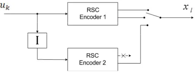
3.1 Turbo encoder

Normally, a Turbo encoder [1] consists of two recursive systematic convolution

(RSC) encoders in parallel, separated by a random interleaver (I). The information

sequences are sent to the first encoder directly, while the second encoder receives the

interleaved information sequences. For code rate r=1 / 3, there is no puncturing, the

code words are 1 2

(x xls, lp,xlp⋅⋅⋅). We could puncture the code words to achieve a higher code rate of ½. In this case, the output code words are 1 2

1 1

( s, p, s , p )

l l l l

x x x₊ x₊ ⋅⋅⋅ .

(19)

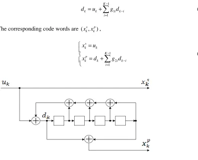
A typical RSC encoder is depicted in Figure 5, where the d is calculated as: k

1 1 1

K

k k i k i i

d u g d

−

− =

= +

∑

(3.1)

The corresponding code words are (x xks, kp),

1 2 1

s k k

K p

k k i k i i

x u

x d g d

−

− =

 ₌

 

= +





∑

(3.2)

Figure 5 RSC encoder

where the feedback generator isg₁i =(11111), and the forward generator isg2i =(10001).

They correspond to octal notation g₁i =37, and g2i =21.

3.2 Maximum a posteriori (MAP) algorithm over AWGN channel

MAP is the optimal symbol-by-symbol maximum a posteriori probability

algorithm [18]. However, MAP is not practical for implementation, primarily because of

the complexity associated with the representation of the probabilities. Log-MAP is a

transform of MAP, and works in the logarithmic domain, which has equivalent

performance and is more practical. We review the fundamentals of MAP/Log-MAP

(20)

11

For an information sequence of length N, we have u=( ,u u1 2,...,uN), where

(0,1)

i

u ∈ , and for the corresponding coded output sequence, we have c =( ,c c₁ ₂,...,c_N), where the length of c is i n for a code rate of r=1 /n. We denote the encoder state at

time i is m . We know that the output and the current state of the convolutional code _i

encoder depend on the previous state and input, so we have the functions:

1

( , )

c

i i i

c = f u m₋ (3.3)

1

( , )

i s i i

m = f u m₋ (3.4)

It is clear that any state pair (m m_i, _i₋₁)corresponds to either u_i =0 or u_i =1. Hence, we have two sets of state pairs S and ₀ S , corresponding to ₁ u_i =0 and u_i =1. Based on observations at the receiver, y=( ,y y1 2,...,yN), we can apply the MAP rule to

find log-likelihood L values as:

1

0

1 1

0 1

( 1| ) ( 1, )

( ) ln ln

( 0 | ) ( 0, )

( , , ) ( , ) ln ln ( , ) ( , , ) i i i i i i i S i i S

P u y P u y

L u

P u y P u y

P m m y P S y

P S y P m m y

− − = = = = = = = =

∑

(3.5)

We define yi( )j =( ...yi yj), where i≤ j. Then we can write

( 1) ( )

1 1

( i , _i, _iN )

y= y − y y₊ (3.6)

(21)

( 1) ( )

1 1 1 1

( 1) ( ) ( 1)

1 1 1 1 1

( 1) ( 1) ( ) ( 1)

1 1 1 1 1 1 1

( 1) 1 1 ( , , ) ( , , , , ) ( , , , ) ( | , , , ) ( , ) ( , | , ) ( | , , , ) ( , ) ( , | i N

i i i i i i

i N i

i i i i i i i

i i N i

i i i i i i i i

i

i i i

p m m y p m m y y y

p m m y y p y m m y y

p m y p m y m y p y m m y y

p m y p m y

− − − + − − − + − − − − − − + − − − = = = = ( ) 1 1

1 1 1

) ( | )

( ) ( , ) ( )

N

i i i

i i i i i i i

m p y m

m m m m

α γ β

− +

− − −

=

(3.7)

where the first three steps follow from the chain rule, the forth step follows from Markov

properties [20], and the last step we define α_i₋₁(m_i₋₁), β_i(m_i), and γ_i(m_i₋₁,m_i) as follows:

( 1)

1 1 1 1

( ) 1 1 1 ( ) ( , ) ( ) ( | ) ( , ) ( , | ) i

i i i

N

i i i i

i i i i i i

m p m y

m p y m

m m p m y m

α β γ − − − − + − − = = = (3.8)

Hence the log-likelihood, L , becomes:

1 1 1 0 1 1 1 0 1 ( , ) 1 ( , )

1 1 1

( , )

1 1 1

( , )

( , , )

( ) ln

( , , ) ( ) ( , ) ( ) ln ( ) ( , ) ( ) i i i i i i i i i i m m S

i

i i m m S

i i i i i i i m m S

p m m y L u

p m m y

m m m m

α γ β α γ β − − − − − ∈ − ∈ − − − ∈ − − − ∈ = =

∑

(3.9)

We can compute αi(mi)forward recursively as following:

1 1 1 1 ( ) 1 ( 1) 1 1

( 1) ( 1)

1 1 1 1

( 1)

1 1 1

( ) ( , ) ( , , , ) ( , ) ( , | , ) ( , ) ( , | ) ( ) ( , ) mi mi mi mi i i i i

i

i i i

S

i i

i i i i

S

i

i i i i

S

i i i i i S

m p m y

p m m y y

p m y p m y m y

p m y p m y m

m m m

α α γ − − − − − − − − − − − − − − − − = = = = =

∑

(3.10)

(22)

13

0 0 0

0

1 0 ( )

0 0 m m m α = = ≠  (3.11)

And we compute βi−1(mi−1) backward recursively as: ( )

1 1

( )

1 1 1

( ) 1 1 1 ( | ) ( , , | ) ( , | ) ( | , , ) ( , | ) ( | ) ( , ) ( ) mi mi mi mi N

i i i

N

i i i i S

N

i i i i i i i S

N i i i i i S

i i i i i S

p y m

p y y m m

p m y m p y m y m

p m y m p y m

m m m

β γ β − − + − − + − − + − = = = = =

∑

(3.12)

assuming that the trellis is terminated in the all-zero state. Hence,

1 0

( )

0 0

N N N N m m m β = = ≠  (3.13)

We compute γ_i(m_i₋₁,m_i) as follows:

1 1 1 1 ( , ) ( , | ) ( | ) ( | , ) ( ) ( | ) ( ) ( | )

i i i i i i

i i i i i i i i

i i i

m m p m y m

p m m p y m m

P u p y u

P u p y c

γ − − − − = = = = (3.14)

The expression clearly shows that γ(m_i₋₁,m_i) depends on the prior probability of the information at time i , and the channel characteristics.

3.3 Turbo decoding over AWGN channel

For an AWGN channel, we have yl = +cl nl. Let us consider the special case

when code rate r=1 / 2, and the systematic convolution code uses BPSK modulation. Under such a condition we have yi =(yis,yip) and ( , )

s p i i i

(23)

need first to calculate the branch metric γi(mi−1,mi).According to formula (3.14), we

further need to calculate the probability of (p y c . _i| )_i

The pdf of y given c could be calculated through its cumulative distribution

function (CDF) as follows:

| ( | )

( | ) y cl l i i

i i

i

F y c

p y c

y ∂ = ∂ (3.15) while | ( | ) ( | ) ( | ) ( | ) ( ) ( ) l l i i

y c i i l i l i l l i l i l i l l i l i i

y c N

F y c P y y c c

P c n y c c

P n y c c c

P n y c

f α αd

− −∞ = ≤ = = + ≤ = = ≤ − = = ≤ − =

_∫

(3.16)

Therefore, we get:

| ( | )

( | )

( )

( ) | ( ) ( )

( ) 0

( )

l l

i i

y c i i i i i y c N i y c

N N i i N

N i i N i i

F y c

p y c

y

f d

y

f f y c f

f y c

α α α − −∞ − −∞ ∂ = ∂ ∂ = ∂ = = − − −∞ = − − = −

∫

(3.17)

where fN( )α is the pdf of the AWGN channel. So the branch metric is:

1

2 2

0 0

2 2 2 2

0 0 0

( , ) ( ) ( | )

( ) ( ) ( )

exp

( ) ( ) ( ) ( ) 2 2

1

exp ( ) exp

i i i i i

s s p p

i i i i i

s p s p s s p p

i i i i i i i i

i

m m P u p y c

P u y c y c

N N

y y c c y c y c

P u

N N N

(24)

15 Because of BPSK modulation, the term

2 2 2 2

0 0

( ) ( ) ( ) ( )

1 exp

s p s p

i i i i

y y c c

N N π  ₊ ₊ ₊  −    

is independent of ui, and it could be cancelled from the numerator and the denominator

of the log-likelihood L values in the formula (3.9), as follows:

1 1

1 0

1 1

( , ) 0

1 1

( , ) 0

1 1

( 0

0

2 2

( ) ( ) exp ( )

( ) ln

2 2

( ) ( ) exp ( )

2

( ) ( ) exp ( )

4 ( 1)

ln ln

( 0)

i i

i

s s p p i i i i

i i i i i

m m S

i _s _s _p _p

i i i i

i i i i i

m m S

p p i i

i i i i i

m

c s i

i

y c y c

m P u m

N L u

y c y c

m P u m

N

y c

m P u m

E P u N

y

N P u

α β α β α β − − − − − ∈ − − ∈ − −  ₊      =  ₊          =   = + + =

∑

1 1 1 0 , ) 1 1

( , ) 0

2

( ) ( ) exp ( )

( ) ( ) i i i m S p p i i

i i i i i

m m S s

c i a i e i

y c

m P u m

N

L y L u L u

α β − ∈ − − ∈       = + +

∑

(3.19)

where we define L as the channel reliability factor [7], c L u is a priori information, a( )i

and L u as the extrinsic information of the systematic bit e( )i s i

y , which is dependent on

the received parity bits.

1 1

1 0

0

1 1

( , ) 0

1 1

( , ) 0

4

( 1)

( ) ln

( 0)

2

( ) ( ) exp ( )

( ) ln

2

( ) ( ) exp ( )

i i i i c c i a i i p p i i

i i i i i

m m S

e i _p _p

i i

i i i i i

m m S

E L N P u L u P u y c

m P u m

N L u

y c

m P u m

N α β α β − − − − ∈ − − ∈ = = = =       =      

∑

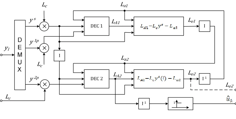
(3.20)

For turbo decoding, corresponding to the turbo encoder, we have two MAP decoders,

DEC1 and DEC2, which iteratively exchange extrinsic information as a priori

(25)

bits y into parallel data bits (l

1 2

, ,

s p p

y y y ). Corresponding to the turbo encoder, the

received systematic bits s

y and parity bits 1 p

y are sent to the first MAP decoder, which

is depicted as DEC1 in Figure 6. The interleaved systematic data bits y i and the s( )

received parity data bits 2 p

y , which are already interleaved at the turbo encoder, are sent

to the second MAP decoder, which is DEC2 depicted in Figure 6.

Figure 6 Turbo decoder

At the first iteration, we do not have the extrinsic information yet, assuming all

bits are equiprobable, and so set a priori probability value L to zero. Thus we get the a1

first extrinsic information L from the first MAP decoder; the superscript represents the (1)_e₁ iteration number of the decoding process.

(1) (1) (1) (1)

1 1 1 1

(1) 1

0

s s

e A c a A c

s A c

L L L y L L L y

L L y

= − − = − −

= − (3.21)

The first extrinsic information L after interleaved, becoming(1)e1 (1)

1( )

e

L I , is sent to

(26)

17

from the first MAP decoder as its a priori probability L of the transmitted data bits. In _a₂

the second decoder, after decoding, we get a new extrinsic information L(1)_e₂:

(1) (1) (1)

2 2 2

(1) (1)

2 1

( )

( ) ( )

s

e A c a

s

A c e

L L L y I L

L L y I L I

= − −

= − − (3.22)

The (1) 2

e

L , after de-interleaved, becoming (1) 1 2( )

e

L I− , is fed back to the first MAP

decoder as its a priori information of the next iteration.

( 2) ( 2) (2)

1 1 1

( 2) (1) 1

1 2( )

s

e A c a

s A c e

L L L y L

L L y L I−

= − −

= − − (3.23)

The general formula for the extrinsic information is as follows:

( ) ( ) ( ) ( ) ( 1) 1

1 1 1 1 2

( ) ( ) ( ) ( ) ( )

2 2 2 2 1

( )

( ) ( ) ( )

i i s i i s i

e A c a A c e

i i s i i s i

e A c a A c e

L L L y L L L y L I

L L L y I L L L y I L I

− −

= − − = − −

= − − = − − (3.24)

with the number of iterations i≥1, and L(1)a1 =L(0)e2 =0. The capital letter I in brackets

represents the interleaver and de-interleaver with a negative power of 1. The whole

decoding process runs iteratively for the given times to improve the decoding

performance.

The upper part and the lower part of the turbo decoder is identical, except that

every piece of information that goes through the lower part must be interleaved and the

output of the lower part must be de-interleaved before using.

At the end of the iterative decoding process, we can make a decision ˆu by _k

comparingLA₂(uk) to a threshold equal to zero,

2 2

ˆ 1 ( ) 0,

ˆ 0 ( ) 0,

k A k

u if L u

= ≥

(27)

From Figure 6, we see that two pieces of information are needed by the turbo

decoder, channel reliability factor L and observations _c y or decision variables. _l

3.4 Turbo decoding over the Rayleigh fading channel

The structure of the turbo decoder over the Rayleigh fading channel is identical to

that over the AWGN channel. From the point of view of the turbo decoder, we still need

two pieces of information, i.e., the channel reliability factor and decision variables.

However, due to the different channel models, we need to modify those two pieces of

information. In [6], the author assumes that there already exists a channel estimator, in

this thesis we call it channel estimator (1). The channel estimator (1), h , is modeled as l

l l l

h = +a m (3.26)

where m is the estimate error of the Rayleigh fading channel _l a , which is complex _l

valued and Gaussian distributed with

2 2

[ ] 0

[| | ] 2

l

l m

E m

E m σ

=

= (3.27)

The estimate error of the estimator (1), m , is independent of the channel l a . l

Further we have:

2 2 2 2

[ ] [ ] [ ] [ ] 0

[| | ] [| | ] [| | ] [| | ]

l l l l l

E h E a m E a E m

= + = + =

= + = + (3.28)

In [6], the author gives the new decision variables z based on the received bits _l

l

y and the estimation h of the channel estimator (1): l

*

l l l

z = y h (3.29)

(28)

19

* 2

2 2 2 2 2 2 2

[ ]

[| | ] [| | ] (| | )( )

l l a l

l

l l l a n a m

E y h c

E y E h c

σ µ σ σ σ σ = + + ≜ _(3.30)

The author of [6] also derived the probability density function of z conditioned on the _l

transmitted code symbol c as follows: _l

*

2 2 2 2

0 2

[ ]

1

( | ) exp

2 (1 | | ) (1 | | )

| | (1 | | )

l l l l

h y y h

l y h

R z p z c

z K µ πσ σ µ σ σ µ σ σ µ   =   − _ − _   × _ _ −   (3.31)

Where K x is the zeroth order Hankel function of o( ) x , and ( )R x denotes the real

component of x . The author of [6] then uses MAP algorithm as mentioned in section

(3.2) to calculate the log likelihood ratio of a posteriori probabilities as follows:

1 1 1 0 1 1 1 0 1 ( , ) 1 ( , )

1 1 1

( , )

1 1 1

( , )

( , , )

( 1| )

( ) ln ln

( 0 | ) ( , , )

( ) ( , ) ( ) ln ( ) ( , ) ( ) i i i i i i i i

i i l m m S

i l i

i l i i l

m m S

i i i i i

m m S

i i i i i

m m S

p m m z

P u z

L u

P u z p m m z

m m m m

α γ β α γ β − − − − − ∈ − ∈ − − − ∈ − − − ∈ = = = = =

∑

(3.32)

Similar to the formula (3.14), the author gets,

1

( , ) ( ) ( | )

i mi mi P u p z ci i i

γ − = (3.3)

Finally, the author of [6] gives out the new channel reliability factor L as follows: _c

1

2 2 2 2

0 0

4 2

( 1)

c s

c a m a a

E E

L

N σ σ N σ σ

−

 

=  + + 

  (3.34)

For a perfect channel estimator (1), 2

(29)

The BER performance may be improved by up to1 dB at a bit error probability of

3

(30)

21 CHAPTER IV

ADAPTIVE TURBO DECODER

The exact turbo decoding metric (3.29) over Rayleigh fading channels assumes

there is an estimator (1) with an estimation error variance of σ_m2. In [6], simulation results show that the smaller the error variance, the better the BER performance. Many

works have been studied to reduce the error variance of the channel estimator (1). Most

of them ignored the extrinsic information (L ) generated during the turbo decoding _e₂ process.

In this Chapter, we first propose a new adaptive algorithm for turbo decoding,

which uses the extrinsic information (L ) and the systematic observations (_e₂ s

y ) as its

inputs. Then we review the basic theory of the estimation. The optimal solutions of

minimum mean square error are modified to become more suitable to the iterative nature

of turbo decoding by combining the steep-decent method. Further, the optimal step size

of the steep-decent algorithm of the Newton’s method is also adapted to the iterative

nature of turbo decoding. At the implementation stage, the stop-and-go strategy makes

the proposed adaptive filter more realistic. The boundary of estimation error variance of

the estimator (2) is also discussed in detail.

4.1 Block diagram of the proposed adaptive filter

We follow the work of author [6]. There are two things that should be noticed.

First, the channel estimator (1) is imperfect; secondly, the channel estimator (1) does not

update iteratively as the Turbo decoder does. In other words, after getting the new

(31)

(1) any more. However, the turbo decoder generates new information about the

transmitted data bits after each iteration. The extrinsic information generated by the turbo

decoder could help us better understand what we have received after each iteration. The

proposed algorithm makes use of this kind of information to re-estimate the channel

adaptively. In this thesis we will call it channel estimator (2), as depicted in Figure 7.

ˆ

_l

a

2 ˆ

m

σ

ˆs c

L

ˆs l

z

Figure 7 Block diagram of adaptive filter

Like in Figure 6, from the point view of the turbo decoder, we summarize two

pieces of information, the decision variables ( z or y ) and the channel reliability factor

(L ), as inputs of the turbo decoder for all the three situations, which are the conventional _c

turbo decoding metric, the exact decoding metric, and the proposed adaptive decoding

metric. Further in Figure 7, we split up these two pieces of information into two sets of

pairs. One set of pair is (zp,L ), which is related to the parity bits, the other is (_cp z L ), s, s_c

which is related to the systematic bits. The superscripts ( ,s p ) represent systematic and

parity bits respectively. The proposed adaptive filter takes both the systematic

(32)

23

the turbo decoder, as its inputs. This is one of the unique choices of this thesis. Some

research takes the hard decision as its input of the adaptive channel filter [13], while

some takes only the soft information as its input of the adaptive filter [14]. None of them

split up the two pieces of information ( ,z L ) into two sets of pairs. The basic motivation _c

to make such kind of choice is that we do not want any delay or memory in the proposed

algorithm. Any delay or register would increase the cost and complexity of the turbo

decoder. Because the length of the extrinsic information is N , which is the same as the

length of the systematic observations, we could simultaneously calculate the updated

channel without any delay or register. We then re-estimate the channel, and finally update

the channel reliability factor and decision variables after each iteration of the turbo

decoding process. Because the extrinsic information generated by the turbo decoder is

only related to the systematic data bits, we only update the channel reliability factors and

the decision variables that are related to the systematic bits. Once we get the updated

channel estimation and its variance, the fading compensator computes out the two

updated pieces of information that the turbo decoder needed as depicted in

Figure 6 and Figure 7, the updated channel reliability factor ˆLs_c and the updated decision

variables ˆz . _ls

4.2 Estimation theory review

According to the theory of estimation discussed in [21], the minimum mean

square error estimator ˆa of the unknown channel a , given observations y , is:

ˆ o

a=w y (4.1)

(33)

1

o

ay y

w =R R− (4.2)

while the covariance Ry and the cross-covariance Ray are defined as follows:

* *

y

ay

R Eyy

R Eay

=

= (4.3)

The solution o

w minimizes the cost function of the channel in the mean square

error sense,

2

ˆ

min ( )

o

w E a−a (4.4)

and the minimum mean square error (m.m.s.e.) is:

1

. . . . _a _ay _y _ya

m m s e =R −R R R− (4.5)

The optimal linear solution o

w is clearly not sensitive to the iterations of the turbo

decoding process in general. In other words, no matter how many iterations we choose,

the optimal minimum mean square error solution remains the same. This also means that

the optimal linear solution o

w is optimal for the whole of the iterations, not for each of

them. If we use the optimal linear solution w directly in the each iteration of the turbo o

decoding process, the turbo decoder must be disturbed at each of the iterations.

The any solution w could also be achieved by the steepest-decent algorithm of o

Newton’s method [21] iteratively, as follows:

1

1 1

1

[ ]

i i y ya y i

w w R R R w

w any initial guess

step size

µ

−

− −

−

 ₌ ₊ ₋



=



 ₌



(4.6)

(34)

25

Because the steep-decent algorithm and the decoding process of the turbo decoder

have such similar iterative characteristics, they could help each other during the decoding

process.

4.3 The proposed estimator (2) of channel a

First we calculate the covariance Ry and the cross-covariance Rayby using the

definition [20] as well as the channel model discussed in chapter 2,

* * 2 2

* * 2

( )( ) 2 2

( ) 2

y a n

ay a c

ya a c

R Eyy E ac n ac n

R Eay Ea ac n m

R Eya E ac n a m

σ σ σ σ = = + + = + = = + = = = + = (4.7)

Then we get the solution to the Newton’s method

1

1 1

2 2 2

1

1 2 2

2 2 2

1

1 2 2

[ ]

[2 (2 2 ) ]

2 2

[ ( ) ]

i i y ya y i

a c a n i i

a n a c a n i i

a n

w w R R R w

m w w m w w µ µ σ σ σ σ σ µ σ σ σ σ σ − − − − − − − = + − − + = + + − + = + + (4.8)

where the mean value of the coded bits (m ) is related to the extrinsic information (c L ). e2

See formula (4.16) later.

The optimal step size µo is calculated as follows [21]:

2 2 max min 2 1 2( ) o a n µ λ λ σ σ = =

+ + (4.9)

where λ_max and λ_min denote the maximum and minimum eigenvalues of the covariance

y

(35)

decoding process as we see in the formula (4.9). Within the limited iterations of the

decoding process, we naturally want to take the biggest step size first then gradually

reduce the step size to reach the fastest convergence. In other words, we need relate the

optimal step size to the iterations of the turbo decoding process in some specific way, as

shown below.

We combine the solution to Newton’s method and the normal equation, as well as

based on the above considerations of the step size, the estimator (2) of the channel a is:

2 2 2

1

1 2 2

1 2 2 ˆ [ ( ) ] ˆ ˆ ˆ ( ) s s

s s s a c a n i

i i i

a n l

a n

m y a

a w y a

a h k i µ σ σ σ σ σ µ σ σ − − −  ₋ ₊ = = +  +  =    ₌ × +  (4.10)

In the above equation, we take the estimation of the estimator (1), both the

systematic and parity bit part, as the initial value of the estimator (2), which is aˆ₋₁=h_l as shown in the formula. The size of the initial value aˆ−1 is n N× with a code rate of

1 /

r= n, while the size of ˆais,mc,wi and s

y is N , which is the length of the information

sequence. After the initialization, we only calculate and update the systematic part ˆa as is

the superscript s indicated. And i is the iterations of the turbo decoder and/or Newton’s

method. Here, we combine them together and make no differentiation between them

afterwards. The step size is reversely proportional to the iteration of the turbo decoder by

practice and the above discussions.

Hence, the minimum mean square error (m.m.s.e.) of the estimator (2) and the

(36)

27

2 2

1 2

2 2

(2 )

. . . . 2

2 2

a c a ay y ya a

a n

m

m m s e R R R R σ σ

σ σ − = − = − + (4.11) 2 2 2 2

ˆ (1 2 2)

a c m a a n m σ σ σ σ σ = − + (4.12)

Finally we get the updated channel reliability factor ˆs c

L and updated decision

variables ˆs l

z ,

1

2 2 2 2

ˆ

0 0

4 2

ˆ ₍ ₁₎

ˆ ˆ

s

s s

c a m a a

s s s l l i

E E

L

N N

z y a

σ σ σ σ −   =  + +    = (4.13)

where the size of ˆs c

L and ˆz is also N , the length of the information sequence. ls

The proposed adaptive decoding metric (4.13) is the same as the one used in the

exact decoding metric (3.29), except that the error variance σm2ˆ is updated iteratively

during the decoding process with the selecting criterion as follows.

2 2 ˆ

m m

σ <σ (4.14)

In the above equations we need to calculate the mean value of the coded bits. By

definition [7], we have

2

( 1) ( 1)

ln ln ln

( 0) ( 1) 1

1

( 1) (1 ) ( 1)

e e k e k L L c

P u P c p

L

P u P c p

e p

e

f pδ c pδ c

= = = = = = − − = + = − + − + ≜ (4.15)

So the mean value of the coded bits is:

2

[ ] ( ) 2 1 tanh( )

2

e

c c

L m E c +∞cf c dc p

−∞

(37)

The mean value of the coded bits is only related to the systematic bits, so we did

not put a superscript s around its right upper corner for simplicity.

One last thing we need to mention is that all the calculations are bit wised in the

formulas. This also means each systematic bit has gone through the channel with

different channel estimations. The square of m in the equation (4.12) is calculated by _c

array power function with the Matlab, and the term s c

m y in the formula (4.10) is

calculated by array multiplication with the Matlab, and so are the array operations in the

other formulas. For simplicity, we did not put another notation around them to avoid

notation confusion. But they should be clear by the context.

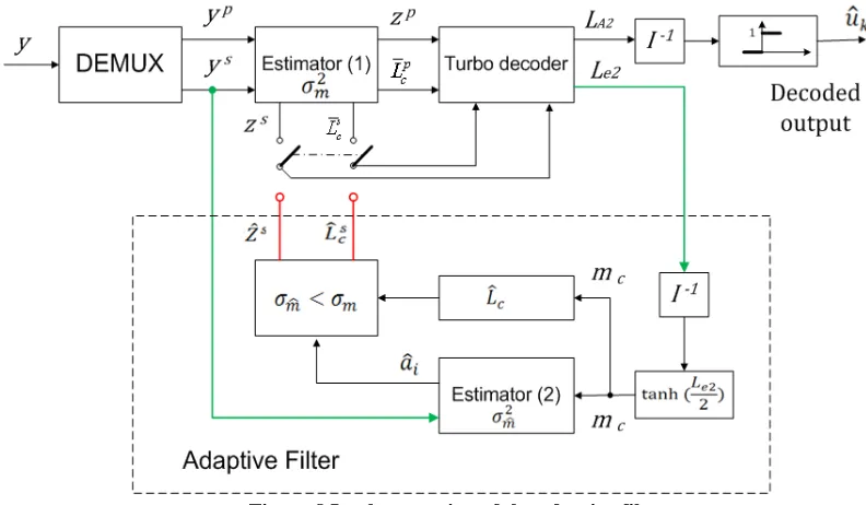
4.4 Implementation of the proposed adaptive filter

Considering the results of the calculation and some practical additions to the

adaptive filter, we construct the adaptive filter as depicted in Figure 8. In the diagram

below, the proposed adaptive filter has two inputs and two outputs.

(38)

29

The two inputs are the extrinsic information from the turbo decoder and the

observations that are related to the systematic bits. The two outputs are the updated

observations and updated new channel reliability factor.

At the first iteration, the received coded data bits go through the estimator (1).

The estimator (1) produces two pieces of information, the new channel reliability factor

c

L and the new decision variables z , that the turbo decoder needed, as depicted in _l

Figure 6. We split these two pieces of information into a systematic part (z Ls, cs) and a

parity part (zp,Lcp). Both systematic part and parity part are the inputs to the turbo

decoder at the first iteration. After the first iteration, we get the extrinsic information

from the turbo decoder, which could help us better understand what we have received

about the transmitted data bits. In the meantime, we toggle the switch to the estimator (2).

The extrinsic information from the turbo decoder is first de-interleaved, and then, by a

simple function, we get the mean value of the systematic bits. Using the mean values we

immediately get the error variances of the updated channel or estimator (2) through the

formula (4.12). After the first iteration, we take the estimation values of the channel from

the channel estimator (1) as the initial guess of the adaptive channels estimator (2). Then

we get the updated channel reliability factor and decision variables by the formula (4.13).

Through practice we compare the error variances of the estimator (2) to the error

variances of estimator (1). We only update the information that has less error variances in

estimator (2). If the error variances or standard derivations of estimator (2) are bigger

than those of estimator (1), we skip further calculation for those bits. The comparison of

the error variances of estimator (1) and estimator (2) provides the proposed adaptive filter

(39)

The extrinsic information from the turbo decoder is only related to the systematic

bits, so we only update the decision variables and the channel reliability factors (z L ) ˆ ,s ˆs_c

that are related to the systematic bits. While the parity part (zp,L ) remains the same cp

during the rest of the decoding iteration process.

4.5 The boundary of estimation error variance of the estimator (2)

The proposed adaptive filter has a selective criterion, as shown in Figure 8 and the

formula (4.14). We rewrite the formula (4.12), (4.14) and (4.16) here for convenience.

2 2 2 2

ˆ (1 2 2)

a c m a

a n

m

σ σ σ

σ σ

= −

+ (4.12)

2 2 ˆ

m m

σ <σ (4.14)

2

[ ] ( ) 2 1 tanh( )

2

e

c c

L m E c +∞cf c dc p

−∞

= =

_∫

= − = (4.16)

The right side of the formula (4.14) is the estimation error variance of the

estimator (1), while the left side is the estimation error variance of the estimator (2),

which varies during the decoding process. We wish to get the smaller error variance of

the adaptive filter. So, the minimum variance or the boundary of the adaptive filter

happens when the mean value of the coded bits reach its maximum. From formula (4.16),

we know that the maximum value of m in the formula (4.12) is 1, so we get the c2

boundary of estimation error variance of the estimator (2) as follows:

2

2 2 2

ˆ 2 2

(1 a )

a m m

a n σ

σ σ σ

σ σ

− < <

(40)

31 which could be further simplified as:

2 2 2 2 ˆ 2 2 a n m m a n σ σ _σ _σ

σ +σ < < (4.18)

After some calculations and from formula (2.1), we get,

2 2 0

( )/10

2 10

a s n SNR dB

N E

r

σ σ = =

× (4.19)

So, we relate the boundary to the signal-to-noise ratio as follows:

2 2 2 ˆ ( )/10 10 a s m m SNR dB s E E r

σ _<_σ _<_σ

+ × (4.20)

With the code rate of r=1 / 2, and setting both 2

a

σ and E_s equal to 1, we get the boundary of estimation error variance of the estimator (2) for the special case,

2 2 ˆ ( )/10

2

2 10+ SNR dB <σm <σm (4.21) 4.6 Decoding method comparison

In this chapter, we derived a new adaptive turbo decoding metric (4.13) for BPSK

signaling on Rayleigh fading channels with the channel estimator (1) providing a certain

error variance.

In some studies, the performance of turbo decoding on Rayleigh fading channels

has also been studied [3], [4] and [22]. In [3], the amplitude and phase of the fading

channels are assumed to be known, and then the Rayleigh fading channel can be modified

as a special case of the AWGN channel conditioned on the known fading factors. In [4],

the phase of the fading channels is assumed to be known and the amplitude is unknown,

then the probability density function (pdf) of the received symbols is adopted

(41)

the conventional decoding metric of AWGN may be used. In [22], the amplitude is

assumed to be constant and the phase is unknown, the decision variables are also

modified approximately as Gaussian and the conventional Turbo decoding metric is used

again. However, in practical communication systems, the channel information is

completely unknown at the receiver, and the fading channels must be estimated at the

receiver. In [6], such an estimator is assumed to provide us with an unbiased channel

estimate with a certain error variance, and the exact decoding metric on Rayleigh fading

channels is derived. In [10] and [11], the exact turbo decoding metric derived in [6] is

simplified with no performance degradation. All the above decoding methods for

Rayleigh fading channels have no feedback from the turbo decoder, while the adaptive

turbo decoding metric derived in this chapter takes the extrinsic information generated

(42)

33 CHAPTER V

SIMULATION RESULTS

5.1 General settings

In the simulation results, two generators of the constituent RSC encoder ( 1 37g = and 2g =21, in octal notation) have been used in Figure 4 and Figure 5. The code rate is

1 / 2

r= , and we set both 2

a

σ and E equal to 1. The channel estimator (1) in Figure 8 is _s simulated. That is, m in the formula (3.26) is generated randomly. The variance of _l m is l

set to 2

0.4

m

σ = in Figure 9 and Figure 11, and the variance of m_l is set to 2

0.4, 0.3,

m σ =

and 0.1 in Figure 10 respectively. The turbo decoder with 8 iterations is used in all

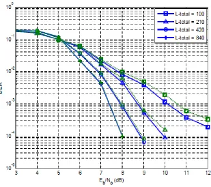
situations. The block length of N =840, 420, 210, and 100 are used in Figure 9 respectively, and the block length of N =100 is used in Figure 10 and Figure 11. 5.2 BER performances with different settings

In Figure 9 and Figure 10, we present the simulation improvements when using

the proposed adaptive filter (solid lines) against the results of Frenger’s (dashed lines) in

[6].

In Figure 9, we consider varying the block sizes of the information sequence. We

can see that, as the block size of the information gets smaller, from N=840 to N=100, the performance of the turbo decoder degrades. The proposed adaptive filter does not

improve the performance much when the information block size isN=840 or greater than that. This could be explained due to the turbo decoder getting more information

from the increased information size, which helps the decoding process. When the

(43)

decoder to achieve better BER performance. Looking at the bit error rate of 3.5 10× −4, we see that the gain of using the proposed adaptive filter is about 1dB for the block length of

100

N = . The improvement of the turbo decoder with the proposed adaptive filter gets bigger when the information block size gets smaller.

Figure 9 BER performance when using adaptive filter (solid) vs the results of Frenger’s (dashed)

In Figure 10, we compare the simulation results of the proposed adaptive filter

(solid lines) versus the results of Frenger’s (dashed lines) in [6] with different error

variances (σm2) of the estimator (1) in Figure 8, while the information block size stays the

same as N =100. When the error variance of the estimator (1) is σm2 =0.1 or less, we see that the proposed adaptive filter gets exactly the same curve with an SNR of less than

8dB. This is because we use the selection criterion as shown in Figure 8 and the formula

(44)

35

selection criterion. If the selection criterion is not satisfied, the proposed adaptive filter

does not update the channel. This could be also explained as the estimator (1) in Figure 8

having already done a better estimation of the fading channels. When the error variance

of the estimator (1) is σm2 =0.4, at the bit error rate of

4

3.5 10× − , we see that the gain of using the proposed adaptive filter is about 1dB . We can see that as the error variance of

the estimator (1) gets bigger, the improvement of the turbo decoder with the estimator (2)

also gets bigger. This means when the channel estimator (1) gets worse, the proposed

channels estimator (2) has more room to improve the BER performance.

Figure 10 BER of the adaptive filter (solid) vs the results of Frenger's (dashed) with different σ2_m

From both Figure 9 and Figure 10, we see that when either the block size of the

(45)

the proposed adaptive filter could help to improve the BER performance of the turbo

decoder.

In comparison, we also give out the simulation results with the settings of

100 N = , 2

0.4

m

σ = and 8 iterations, but do not compare the error variance of the

estimator (2) to those of the estimator (1). That is, there is no selecting criterion (σm2ˆ <σm2)

for the adaptive filter in Figure 8. The adaptive filter does not provide better performance

in this case.

1 2 3 4 5 6 7 8 9 10 11 12 10-4

10-3 10-2 10-1 100

SNR (dB)

B

E

R

L-total = 100 ( No Selecting )

No Select (1:12,8) Frenger (1:12,8)

Figure 11 BER without selecting criteria

5.3 Step size and boundary

The step size of the steep-decent algorithm for the proposed adaptive filter, see

formula (4.10), is depicted in Figure 12. Please note that the formula (4.10) follows the

general convention of the steep-decent algorithm. The initial guess of the channel aˆ−1 is

(46)

37

formula (4.10) begins to vary from iteration 2 of the decoding process. The adaptive

channel estimator (2) in Figure 8 takes its biggest step at the iteration 2 of the decoding

process to accelerate convergence, and then reduces the step size reversely to the

iterations.

Figure 12 Step size versus iterations

In Figure 13, the boundary of estimation error variance of the estimator (2) for the

special case is given according to the formula (4.21). That is, the code rate r=1 / 2, and both σa2 and E are set to 1. The arrow area is an example of the boundary with the s

estimation error variance σm2 =0.4 of the estimator (1). The arrow area shows that the adaptive filter starts to improve BER after SNR greater than 6dB when σm2 =0.4, the bigger SNR, the larger distance from 2

0.4

m

σ = to the lower boundary. This means more ability to improve the BER performance. This could be verified by the BER

(47)

to improve the BER after SNR greater than 7dB, and when σm2 is 0.1, the adaptive filter

does not improve the BER before SNR greater than 13dB. These could also be verified

by the BER performances with different settings in Figure 10.