An Efficient 3D Imaging using Structured Light Systems.

(1)

ABSTRACT

LEE, DEOKWOO. An Efficient 3D Imaging using Structured Light Systems. (Under the direction of Dr. Hamid Krim.)

Structured light 3D surface imaging has been crucial in the fields of image processing and computer vision, particularly in reconstruction, recognition and others. In this dis-sertation, we propose the approaches to development of an efficient 3D surface imaging system using structured light patterns including reconstruction, recognition and sam-pling criterion. To achieve an efficient reconstruction system, we address the problem in its many dimensions. In the first, we extract geometric 3D coordinates of an object which is illuminated by a set of concentric circular patterns and reflected to a 2D im-age plane. The relationship between the original and the deformed shape of the light patterns due to a surface shape provides sufficient 3D coordinates information. In the second, we consider system efficiency. The efficiency, which can be quantified by the size of data, is improved by reducing the number of circular patterns to be projected onto an object of interest. Akin to the Shannon-Nyquist Sampling Theorem, we derive the mini-mum number of circular patterns which sufficiently represents the target object with no considerable information loss. Specific geometric information (e.g. the highest curvature) of an object is key to deriving the minimum sampling density. In the third, the object, represented using the minimum number of patterns, has incomplete color information (i.e. color information is given a priori along with the curves). An interpolation is car-ried out to complete the photometric reconstruction. The results can be approximately reconstructed because the minimum number of the patterns may not exactly reconstruct the original object. But the result does not show considerable information loss, and the performance of an approximate reconstruction is evaluated by performing recognition or classification.

(2)

methods and non-linear methods have been investigated for a dimensional reduction which achieves efficient recognition / classification algorithms. But, existing approaches generate many parameters which leads to an optimization procedures which sometimes do not provide explicit solution. The proposed approach to dimensionality reduction for recognition is based on the property of theFourier Transform whose magnitude response is symmetric and invariant to time-shift, and the results are much more explicit without loss of intrinsic information of targets.

(3)

(4)

An Efficient 3D Imaging using Structured Light Systems

by Deokwoo Lee

A dissertation submitted to the Graduate Faculty of North Carolina State University

in partial fulfillment of the requirements for the Degree of

Doctor of Philosophy

Electrical Engineering

Raleigh, North Carolina

2012

APPROVED BY:

Dr. Griff L. Bilbro Dr. Wesley E. Snyder

Dr. Larry K. Norris Dr. Hamid Krim

(5)

DEDICATION

(6)

BIOGRAPHY

(7)

ACKNOWLEDGEMENTS

I would never been able to complete my M.S and Ph.D degree without help from many people. First of all, I would like to thank my advisor, Dr. Hamid Krim. I will not forget his financial support, his academic advice, his insight and his unlimited patience with my graduate research. In addition, his support could make my Ph.D work complete and guided me in the right way to research goal and my future career.

I also would like to thank my advisory committee members, Dr. Griff Bilbro, Dr. Wesley Snyder, Dr. Larry Norris and Dr. Michael Escuti. I also would like to thank Dr. Brian Hughes, Dr. Cranos Williams, Dr. Alexandra Duel-Hallen, Dr. Dror Baron and Dr. Keith Townsend. I also would like to thank and am proud of my former / current VISSTA group members including visiting students and scholars, Alex Chen, Djamila Aouada, Sheng Yi, Harish Kumar, Scott Clouse, Jennifer Gamble, Adam Wilkerson, Glenwood Garner, Xiao Bian, Tian Wang, Cesare Ceozzi, Nath Anh, Jaime, David, Axel and Heill Han (visiting Professor).

I also would like to thank the Korean students and Professors at North Carolina State University and in RTP area. I am also very grateful to the Professors in South Korea, Dr. Yeongho Ha, Dr. Eonkyung Joo, Dr. Jaekeun Hong, Dr. Kangwook Kim and Dr. Chunpyo Hong, who supported and encouraged me to study in the United States.

(8)

LIST OF TABLES

(12)

LIST OF FIGURES

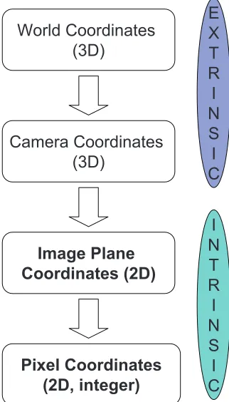
Figure 1.1 Overall calibration process. Prior to 3D reconstruction from 2D images, we need to align two coordinate systems. The first one is between world coordinate and camera coordinate system. The second one is between real coordinate and pixel coordinate system. The former one is related to estimating extrinsic parameters and the latter one is related to estimating intrinsic parameters. . . 3 Figure 1.2 The projective geometry of a pinhole camera model. . . 5 Figure 1.3 Transformation from world coordinates to camera coordinates. This

transformation provides information of extrinsic parameters of a camera. . . 7 Figure 1.4 Since the coordinate systems of 2D image plane (pixel coordinates)

and of the real object space are different, we need to align those coordinate system. . . 9 Figure 1.5 Using 2 cameras, the passive method is based on the triangulation

for 3D reconstruction. . . 12 Figure 1.6 The point M, the optical centers C and C′_{, and the two images} _m

and m′ _of _M _{all lie in the same plane. . . .} ₁₂

Figure 1.7 In general case, a 3D reconstruction activity requires several view-points when a passive method is adopted. . . 14 Figure 1.8 Basic principle of the active method. . . 16 Figure 1.9 Active method using stripe patterns. . . 17 Figure 1.10 An example of a 3D reconstruction using stripe patterns [109]. . . 18 Figure 1.11 A geometrical relationship is a basic principle for a 3D

reconstruc-tion task in an active imaging [37]. B : Distance between center point of a light source and the optical center. R: Distance between the optical center and an object point. . . 19 Figure 1.12 To alleviate drawbacks of stripe patterns, codes are assigned to

each pattern. . . 19 Figure 1.13 To improve efficiency of coded structured light patterns, more

com-plex patterns, such as gray-level or color coded patterns are em-ployed [109]. . . 20 Figure 1.14 Example of a phase shift with three light patterns [37]. . . 21 Figure 1.15 Example of a an experimental setup for 3D measurement using a

structured light system [37]. . . 22 Figure 1.16 Example of a hybrid version of a combination of phase shift and

coded light patterns [37]. . . 23

(13)

Figure 1.18 A system (generally, static or dynamic) with inputx(t) and output

y(t) is defined as the ratio of the output to input in frequency,

Laplace or Z domain. . . 29

Figure 1.19 In communication theory, the modulation-demodulation theory is used to estimate the user(s) or transmitted signals from the output signal(s) using carrier signal, cosωt. . . 30

Figure 2.1 Ideal and deformed circles. . . 39

Figure 2.2 Ideal and projected(observed) circular patterns. . . 40

Figure 2.3 Setup of structured light projection system using LC2002. . . 41

Figure 2.4 Block diagram of an overall system. . . 41

Figure 2.5 Geometrical representation of domains of the light source, 3D sur-face and 2D image plane. . . 43

Figure 2.6 Reconstruction experimental setup based on parallel projection . . 45

Figure 2.7 (X₋Z) and (Y ₋Z) domain analysis . . . 46

Figure 2.8 Simulation of a profiling zwij coordinates(relative depths) of a red line . . . 49

Figure 2.9 Reconstructed 3D face from a measurement of 3D coordinates (xw, yw, zw) 49 Figure 2.10 Reconstruction example of a terrain model . . . 49

Figure 2.11 Reconstruction examples of a cubic and a penguin model(depth recovery) . . . 50

Figure 3.1 Position of each curve. . . 54

Figure 3.2 Block diagram of light projection and reflection. . . 55

Figure 3.3 Simulated reconstruction example of a small cubic model. . . 56

Figure 3.4 Deformation shape of the projected light patterns are identical on the object which has zero Gaussian curvature. In this case we can reduce the number of light patterns for reconstruction. . . 57

Figure 3.5 Geometry of measurement set up. . . 57

Figure 3.6 Light projection and principal direction of a 3D object. . . 60

Figure 3.7 Principal direction of a 2D curve. . . 62

Figure 4.1 Fourier transform of sampled signal(FromNational Semiconductor Corporation) . . . 68

Figure 4.2 Example of estimation of curvature(left) and variation of curva-ture(right) . . . 70

Figure 4.3 Reconstruction results using 3,4,5 and 9 sampling rates. . . 70

Figure 4.4 i and j respectively index the number of points(M) in each pat-terns, and the pattern’s position.. . . 74 Figure 4.5 Indices of the location of each curve alternatively represented as

(14)

Figure 4.6 In practical perspective (i.e. N is sufficiently large), pattern-wise sampling (e.g. circular patterns) is more efficient than point-wise sampling in aspect of computational complexity and user running time, etc. . . 78 Figure 4.7 The Two-Thirds Power Law explains a relationship between a

ge-ometrical information (i.e. curvature) and an angular velocity of a curve. Angular velocity is composed of a radius r and an angular frequency ω. . . 79 Figure 4.8 For a 3D signal (i.e. surface), at any point Pij, if two orthogonal

tangent vectors are selected, then two corresponding curvatures are defined as well. (a) 3D face model overlaid with projected circular light patterns,(b) 3D pointPij,(c) Two orthogonal tangent vectors

atPij . . . 81

Figure 4.9 θ(i) and ϕ(i) denote the angle between the lines γ(i₋1)γ(i) and

γ(i)γ(i+ 1) and the cumulative angle, (ϕ(i) = ϕ(i −1) +θ(i)), respectively. Geometric properties of a curve and the angles lead to establishment of an algorithm for our sampling frequency. . . . 86 Figure 4.10 Optional caption for list of figures . . . 90 Figure 4.11 Geometric representation of face models(vertices and triangular

faces), Left : Brian, Right : Eric . . . 91 Figure 4.12 Geometric representation of face models(vertices and triangular

faces), Left : Greg, Right : Jeff . . . 91 Figure 4.13 Geometric representation of face models(vertices and triangular

faces), Weihong . . . 92 Figure 4.14 A triangular mesh representation is composed of vertices and faces,

faces being composed of three vertices and a vertex being a 3D coordinate point of a 3D image. Although (f) and (g) are different datasets (i.e. These two figures are simple example datasets for a simulation), these are also used to substantiate our algorithms simply from smaller size of data, and also shorten running time for simulations. . . 93 Figure 4.15 Geometric characteristics of a surface determines the initial number(N)

of circular patterns on a surface. N of an each surface : (a) 147, (b) 153, (c) 142, (d) 221, (e) 271, (f) 89, (g) 93. . . 94 Figure 4.16 Faces with a Curveling rate is corresponding to a subspace of a

(15)

Figure 4.17 Subsurfaces composed ofNscurves (((a) - (e)) shows reliable

recon-struction results in geometric perspective ((f) - (j)). Interpolation starts with color information which is mapped to each curve. From comparison with the original geometric images, there is no consid-erable geometry information loss. . . 96 Figure 4.18 Non-diagonal elements of the correlation matrices provide the

in-formation of similarity, which is the performance of reconstructions. 97 Figure 4.19 Correlation coefficient is calculated between the original face model

and the face model represented using varying sampling density. When the sampling density is below the curveling rate, 0.44, simi-larity is decreased. . . 97

Figure 5.1 In case of a RGB scale images, each coordinate (point, pixel or voxel) is composed of red, green and blue component . . . 102 Figure 5.2 Optional caption for list of figures . . . 103 Figure 5.3 Optional caption for list of figures . . . 104 Figure 5.4 The average of the nearest neighboring samples is calculated to

interpolate color information of a surface. In this case, the number of the nearest neighboring samples isL= 4. . . 105 Figure 5.5 Simulation of projection of circular patterns, (a). 3D face model,

(b). Circular patterns, (c). Overlaying patterns . . . 108 Figure 5.6 Images can be represented by binary scale (C = 0,1), greyscale or

RGBscale. 5 faces are composed of basic color elements, red, green and blue. The first row : Red, The second row : Green, The third row : Blue . . . 109 Figure 5.7 RGB scale faces with a Curveling rate (i.e. The faces are

repre-sented using the minimum sampling density), which is referred to as subsurfaces or subfaces, show some information loss and hence need to be interpolated. . . 110 Figure 5.8 RGB scale faces with a Curveling rate, which is referred to as

sub-surfaces or subfaces, show some information loss and hence need to be interpolated. Mean value of the nearest neighborhood is cal-culated to interpolate a given subface . . . 111 Figure 5.9 RGB scale faces with a Curveling rate, which is referred to as

sub-surfaces or subfaces, show some information loss and hence need to be interpolated. Mean value of the nearest neighborhood is cal-culated to interpolate a given subface . . . 112 Figure 5.10 RGB scale faces with a Curveling rate, which is referred to as

(16)

Figure 5.11 RGB scale faces with a Curveling rate, which is referred to as sub-surfaces or subfaces, show some information loss and hence need to be interpolated. Mean value of the nearest neighborhood is

cal-culated to interpolate a given subface . . . 114

Figure 5.12 RGB scale faces with a Curveling rate, which is referred to as sub-surfaces or subfaces, show some information loss and hence need to be interpolated. Mean value of the nearest neighborhood is cal-culated to interpolate a given subface . . . 115

Figure 6.1 Simple box model. To explain projection constraints, simple model is chosen for an example. Target scene is the area in black lines. Different views are displayed to show how the target is shaped. . . 120

Figure 6.2 (a). Projected area. (b). False projection. When the orientation of a structured light pattern is same as the tangent direction of an object, the pattern is not projected onto the area of an object. This case is referred to as aFalse projection . . . 121

Figure 6.3 Reconstruction using MPV is combining all the reconstruction re-sults followed by coordinate transformation and redundancy elim-ination. . . 126

Figure 6.4 Under the assumption that the object is illuminated only by the projected light patterns, the areas overlaid with overlapped light patterns of different intensities from other areas. From the intensity variations, overlapped patterns are detected. . . 129

Figure 6.5 Viewpoint constraint is a position planning of cameras to com-pletely cover whole object. To achieve an efficient position plan-ning (i.e. minimize the number of viewpoints), maximum distance between neighboring cameras are estimated. . . 130

Figure 6.6 A box model illuminated by 2 projectors each of which generates 7 circular patterns, and 2 cameras capture the patterned image from the left and right perspective of view. The figures in the second row are reconstructed results from each viewpoint. . . 133

Figure 6.7 3 circular patterns are used in our experiment. Radii of these are 1, 2 and 4inches respectively. . . 134

Figure 6.8 Reconstruction is performed from the different viewpoints. . . 134

Figure 6.9 Redundant information is eliminated based on the intensity varia-tions. . . 135

Figure 6.10 Coordinate transformation complete the reconstruction. . . 135

Figure 6.11 Reconstruction of a box model in Fig. 6.1. . . 135

Figure 6.12 Reconstruction of a terrain model. . . 136

(17)

Figure 7.1 A system (generally, static or dynamic) with inputx(t) and output

y(t) is defined as the ratio of the output to input in frequency, Laplace or Z domain. . . 141 Figure 7.2 In communication system, the modulation-demodulation theory is

used to detect the user(s) or transmitted signals from the output signal(s) using carrier signal, cosωt. . . 142 Figure 7.3 A face model is illuminated by a set of cocentric circular patterns.

Given the information of the original circular patterns, deformed circular patterns provides sufficient information to recover 3D real world coordinates of the face model. . . 144 Figure 7.4 According to Thales’ Theorem, and using circular patterns, the

relationship between 3D and 2D points is established. . . 146 Figure 7.5 Instead of Fourier, Laplace or Z domain, our system is defined in

the domain of the position of a circular pattern. . . 147 Figure 7.6 Radius of a projected circular pattern is used to estimate a depth of

an object and the reconstruction system can be represented using a communication system. . . 150 Figure 7.7 Reconstruction of a terrain model. . . 151 Figure 7.8 The observed scene is composed of the target object overlaid with

circular patterns. Akin to demodulation of communication system for estimating transmitted signals, the input, 3D object from each viewpoint, is estimated using projected circular patterns. . . 152 Figure 7.9 The observed scene is composed of the target object overlaid with

circular patterns. Once each observed scene is demodulated by the same circular patterns, 3D coordinates of the target is achieved. . 153

Figure 8.1 The geodesic distance is more proper than the Euclidean distance to represent the intrinsic properties of a generic surface. . . 159 Figure 8.2 Geometrical representation of the experimental setup. 3D

recon-struction (P3) from a 2D image using structured light systems is solved based on establishing a relationship betweenPLandP2. Our

facial curves are deformed circular patterns projected onto a target object. . . 160 Figure 8.3 Original circles are deformed when projected onto an object surface.

Under the assumption of parallel projection, the constraint ofxand

y is preserved. . . 161 Figure 8.4 A set of deformed circular curves represents a surface S, and the

shortest geodesic distance is measured between the reference point

PRand any pointPij on thejthcurve. This figure shows an example

(18)

Figure 8.5 In case of a planar surface, projected circular patterns preserve their shapes, and fDP(x) is a summation of unit step functions. This figure shows an example ofN = 8 andM = 10. . . 166 Figure 8.6 In case of a nonplanar surface, projected circular patterns do not

preserve their shapes, and fD(x) is not a summation of unit step

functions. The face model is represented using vertices and trian-gular faces. Facial curves are extracted based on Eq. (8.2). Bottom :fD(x) shows greater variance compared to fDP(x) in Fig. 8.5 due to the surface shape. . . 167 Figure 8.7 The magnitude of theFourier transform offD(x) shows symmetric

property becausefD(x) is a real value function. . . 168

Figure 8.8 Due to symmetry, the first half of the magnitude of FD(ω) or the

Inverse Fourier Transform of FD(ω) (ω ∈ [0, π)) sufficiently

pro-vide the information about an object. Top : [_|FD(ω)|]πω=0, Bottom :|ef(x)|. . . 169 Figure 8.9 (a) Original face, (b) Geometric representation of a face(a), (c)

Extracted facial curves which are deformed circular patterns. . . . 172 Figure 8.10 Extracted facial curves from the face models. (A) and (B) : Same

face with different expressions, (C) and (D) : Different face models. 173 Figure 8.11 1-(a)–1-(d) : fD(x) of the same person with four different

expres-sions. 2–5 : fD(x) of four different people faces. fD(x)’s are

one-dimensional functions corresponding to the faces in Fig. 8.10. 1-(a)–1-(d)s are functions on the same person with different expres-sions and 2–5 are functions on the different people. We can see that

fD(x)s from the same person have similar shapes, andfD(x)s from

the different persons does not have similar shape, because each function contains the shortest geodesic distance information which is preserved. . . 174 Figure 8.12 Left top : FD(ω), Fourier transform offD(x), Left bottom :

Mag-nitude response of FD(ω), Right top : FfD(ω), the first half of the

magnitude response of FD(ω), Right bottom : ef(x), the inverse

Fourier transform of FfD(ω). . . 175

Figure 8.13 Left top : FD(ω), Fourier transform offD(x), Left bottom :

(19)

Figure 8.16 8 faces with 5 persons (classes) are used to measure the similarity. The similarity quantities (σ12) between the same class (shaded area) are higher than the ones between different classes. . . 179 Figure 8.17 If the classification is carried out using the Euclidean coordinates

directly, the classification result may not provide sufficient informa-tion, because coordinates alignment and scaling factor adjustment should be performeda priori, and these are sometimes inaccurate. 180 Figure 8.18 Classification matrix is composed of σ12’s, by calculating the

cor-relation coefficient matrices between all pairs of the faces. Higher sampling density shows better recognition results. . . 181 Figure 8.19 Classification matrix is composed of σ12s by calculating the

(20)

Chapter 1 Introduction

(21)

error evaluation, we choose to evaluate it by way of object classification and recognition. This is particularly true in practice when ground-truth models may no be available. We particularly carry out a thorough experiment using 3D human face represented by facial curves. In this chapter, we review some background in 3D analysis and geometries, and the relationships between 2D and 3D imaging.

1.1 Projective Geometry

We briefly review, in this section, projective geometry [76] and revisit some fundamental principles in 3D geometric reconstruction work. To reproduce real world information (i.e. 3D coordinates) from 2D images captured by cameras or human vision, projective geometry is best suited than Euclidean geometry. By establishing a relationship between a 3D point of of an object in the real world and a 2D point captured by viewpoint, 3D geometric information is extracted. To establish a geometric relationship, the locations of optical centers of cameras are required a priori. In addition, a coordinate system alignment between a real world object and the camera is very important to generate a simple and efficient mathematical model to measure 3D information. In addition, the coordinate system of a camera or an object and its image plane (i.e. pixel coordinate) should also be aligned prior to the reconstruction procedure.

A camera captures two dimensional images of three dimensional real world objects. Perspective view of an object using geometry, can represent the real 3D world object based on basic principles. These principles constitute the essence of 3D vision techniques such as projective, affine and Euclidean geometries. In addition, these principles are fundamental and crucial to understanding camera calibration process consisting of esti-mating extrinsic and intrinsic parameters (Section 1.2). A pinhole camera model is widely used to understand the camera geometry which implies a transformation (T) from a 3D space (Π⊂R3_{) to a 2D image plane space (}_π_⊂_R2_).

π=_TΠ. (1.1)

(22)

World Coordinates (3D)

Camera Coordinates (3D)

Image Plane Coordinates (2D)

Pixel Coordinates (2D, integer)

E X T R I N S I C

I N T R I N S I C

(23)

a projection from a 3D space to a 2D image plane is composed of an image plane (also called a retinar plane), an optical center C (C does not belong to retinar plane) and a focal length f which is the distance between C and the image plane. The line from C to

cgenerates an axis called optical axis. Once a 3D object coordinate system is completely aligned to a camera coordinate system, we define Mc ∈R3 andm ∈R2 as real world 3D

points and reflected 2D points in the image plane respectively,

Mc = (Xc, Yc, Zc),

m = (u, v).

Although Euclidean Geometry provides a good representation of 2D images reflected from 3D objects, projective geometry is a more adopted approach when we consider a real perspective (e.g. a vanishing point, a point at the infinite distance, etc.).

Definition [76] The projective space of dimension n, denoted Pn _or _P₍_E

n+1) is

obtained by taking the quotient of an n + 1-dimensional vector space En+1 (real or complex), minus the null vector 0n+1, with respect to the equivalence relation

x≅_x′ _{⇔ ∃}_λ₆_{= 0}_, _x₌_λ_x′_,

E : a vector space defined on a fieldK ₍K₌R_,_{the set of real numbers or}

K₌C_,_{the set of complex numbers)}_.

En indicates that En is a vector space of dimensionn.

Using projective geometry (Fig. 1.2), Mc and m may be rewritten as

Mc = (Xc, Yc, Yc,1),

m = (u, v, f).

(24)

Retinar plane

C : Optical center

M

_c

: Real world position

m : point in an image

M_c Z Y Z u v c m f C

Figure 1.2: The projective geometry of a pinhole camera model.

following relationships :

u=fXc Zc

, v =fYc Zc

. (1.2)

The focal length, f determines a scaling of the projected image of a real object. The relationship between Mc and m is linear,m =P0Mc (P0 is called a projection matrix) ;

   u v f   =   

f /Zc 0 0 0

0 f /Zc 0 0

0 0 f /Zc 0

         Xc Yc Zc 1     

. (1.3)

(25)

1.2 Camera Calibration

To solve 3D reconstruction problems, a camera calibration is a necessary and crucial step to determining its intrinsic and extrinsic characteristics and subsequently capturing real objects for reconstruction. To estimate the intrinsic parameters such asfocal length, image center or optical center, together with the extrinsic parameters, provides the necessary information for a coordinate system alignment, and has been extensively researched in 3D computer vision ([98, 124]).

1.2.1 Extrinsic Parameters

In the previous section, we generated a projection matrix by deriving the relationship between 3D points and the reflected 2D points in the image plane. This derivation as-sumed that the world coordinates and the camera coordinates are completely aligned. In practice, however, we need to align these coordinate systems as the camera and the object may not be in the same coordinate systems (Fig. 1.3). Let Mw represent the 3D

coordinates of a point on an object which is defined in the real world coordinate system.

Mw and Mc satisfy the following ;

Mc =R(Mw−T), (1.4)

where R is a 3×3 rotation matrix, and Tis a 3×1 translation vector .

R=

  

r11 r12 r13

r21 r22 r23

r31 r32 r33

  , T=

   TX TY TZ  

. (1.5)

Given R and T above, then

   Xc Yc Zc   =   

r11 r12 r13

r21 r22 r23

r31 r32 r33

     

Xw−TX

Yw−TY

Zw−TZ

 

(26)

0_F

P

&

I _<

F

;_F =_F

<_F

;_F =F

<Z _;

Z

=_Z 0_Z

44QVCVKQP 66TCPUNCVKQP

%COGTC %QQTFKPCVG 5[UVGO

9QTNF %QQTFKPCVG 5[UVGO

57

(27)

or

Xc =RT1(Mw−T),

Yc =RT2(Mw−T),

Zc =RT3(Mw−T), (1.7)

where RT

i is the i−th row of the rotation matrix. Given the relationship between Mw

andMc,RandTare referred to as the extrinsic parameters [109] of a camera, and these

uniquely define the camera reference frame and the world reference frame.

1.2.2 Intrinsic Parameters

Using Eq. (1.2) – (1.7), the perspective projection may be written as

u=fXc Zc

=fR

T

1(Mw−T)

RT

3(Mw−T)

, (1.8)

v =fYc Zc

=fR

T

2(Mw−T)

RT

3(Mw−T)

. (1.9)

In practice, the points of the captured image is represented bypixel coordinates (Fig. 1.4). Letmim be a 2D point defined in pixel coordinates, and written as

mim = (uim, vim). (1.10)

Intrinsic parameters explain the relationship between 2D real coordinatem = (u, v) and the pixel coordinate mim = (uim, vim). Since the pixel coordinates start from the left

corner,m is represented as

u = (uim−u0)αu,

(28)

0 P & I

X

_LP

X

Y

PXYKOCIGEGPVGT

P

Y

_LP

Figure 1.4: Since the coordinate systems of 2D image plane (pixel coordinates) and of the real object space are different, we need to align those coordinate system.

where (uo, vo) is a location of an image center pixel, and αu and αv represent a length

per pixel in horizontal and vertical direction respectively. Using a matrix, Eq. (1.11) is represented as follows :

mim = Am, (1.12)

   uim vim f    =   

−1/αu 0 u0/f 0 −1/αv v0/f

0 0 1

      u v f  

, (1.13)

where the components of the matrix A are called the intrinsic parameters of a camera [109]. Using all above relationships, we can establish a relationship between mim and the

real world coordinates Mw :

mim =AP0DMw, (1.14)

(29)

QR Decomposition [23] Let A be an m×n full column rank matrix with m ≥ n, then A is decomposed into am_×n orthogonal matrixQ and ann_×n upper triangular matrix R with diagonals rii >0. We can writeA as

A=QR,

QTQ=In.

When employing a pinhole camera model, there are constraints when solving the cor-respondence problem, such as epipolar ortrilinear constraints. Lens distortion is a factor which makes it hard for the constraints to hold exactly. One of the internal characteristics of a camera to be considered is a lens distortion which is a significant factor affecting the performance of 3D reconstruction [92]. Observed image points in a 2D image plane are distorted by the optics of a camera lens. Among the numerous lens distortions, the most widely used model is the radial distortion. The mathematical model of the radial distortion establishes the relationships [105] between (ud, vd) and (uu, vu), the distorted

and undistorted data points in a 2D image plane, as follows.

uu = ud+ (ud−uc)(k1r2 +k2r4+. . .) + (P1(r2+ 2(ud−uc)2

+2P2(ud−uc)(vd−vc))(1 +P3r2+. . .),

vu = vd+ (vd−vc)(k1r2+k2r4+. . .) + (P1(r2+ 2(vd−vc)2

+2P2(ud−uc)(vd−vc))(1 +P3r2+. . .), (1.15)

where all the notations above are detailed as :

r=p(ud−uc)2+ (vd−vc)2,

(uu, vu) : Undistorted image point,

(ud, vd) : Distorted image point,

(uc, vc) : Distortion center,

kn:nth radial distortion coefficient,

(30)

Assuming that the radial distortion is dominated by the low order components, and the distortion center is located at (uc, vc) = (0,0), Eq. (1.15) is rewritten as

uu = ud(1 +k1r2+k2r4),

vu = vd(1 +k1r2+k2r4). (1.16)

All of the above relations summarize the essence of projective geometry, and are crucial to 3D reconstruction algorithms for the passive and the active imaging methods as discussed in the next section.

1.3 3D Reconstruction - Passive Stereo Vision

A 3D reconstruction from 2D points in an image plane is based on analyzing the geomet-rical relationships between multiple viewpoints (i.e. cameras) and an object (Fig. 1.5). Recalling the relationship between m _∈ R2 _and _M _∈ R3 _{from Section 1.1, the passive}

method will use 2 or more viewpoints, and we consider 2 viewpoints here. Given 2 cap-tured images, we have mandm′_{. Using the perspective projection, we have the following}

relationships :

m =PMw,

m′ =_P′Mw, (1.17)

where P and P′ _{are projection matrices defined for the first and the second viewpoints,}

respectively. A 3D reconstruction using the passive method solves a correspondence be-tween m and m′_{, where} _m _and _m′ _{belong to different image planes, as reflected points}

of the same 3D point Mw. The Epipolar constraint explains the relationship between m

(31)

M

Z

Y

Z

u

v

c

m

f

C

m’

C’

Figure 1.5: Using 2 cameras, the passive method is based on the triangulation for 3D reconstruction.

C

C’

M

e

m

m’

Figure 1.6: The point M, the optical centers C and C′, and the two images m and m′

(32)

points satisfy the following :

−

→_T ₌−−→

OC′ ₋−−→OC,

−−→

Lm′ =R(−→L_m−−→T), (1.18)

R(−→Lm−−→T),(−→T ×−→Lm)

=0, (1.19)

R−−→Lm′,(−→T×−→L_m)

=0, (1.20)

(RT−−→Lm′)T(−→T ×−→Lm) =0, (1.21)

− →

T _×−→Lm =S−→Lm, (1.22)

(RT−−→_L

m′)TS−→L_m =−−→L_m′TRS−→L_m =0, (1.23) −

→

T = (TX, TY, TZ),

S=

  

0 ₋TZ TY

TZ 0 −TX

−TY TX 0

  ,

where ’<, >’ and ’×’ respectively denote an inner product and a cross product, R is a rotation matrix, E = RS is called the Essential matrix. For clarity, all of the vectors are defined related to the origin point O = (0,0,0) (e.g. −→C = −→OC). If we use the pixel coordinate, 2D coordinates of m and m′ _{are written as}

mim=Mm,

m′im =M′m′,

where M and M′ _{are matrices composed of intrinsic parameters of two cameras. The}

equation −−→Lm′TRS−→L_m =0 is then rewritten as

−−→

Km′ =

−−→

C′m′,

−−→

Km =−−→Cm,

−−→

KTm′F

−−→

Km =0 (1.24)

(33)

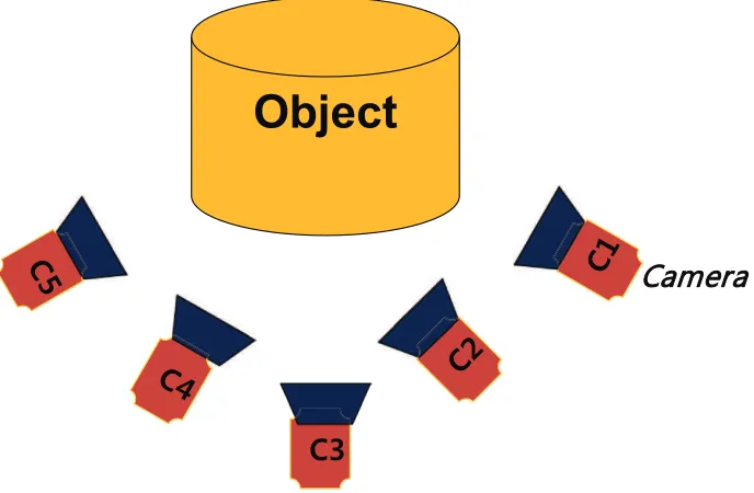
Object

%

&DPHUD

Figure 1.7: In general case, a 3D reconstruction activity requires several viewpoints when a passive method is adopted.

The matrix F is called the Fundamental matrix. Using the Epipolar constraint, we can get a relationship between m and m′ _(i.e. _m ₌_H_m′_{), where} _H _{represents the}

relation-ship between m and m′ _{which are 2D reflected points of the same object point} _M_{, and}

solve the 3D reconstruction problem. In general perspective, we can use the algorithms above to solve the reconstruction problem with several viewpoints (Fig. 1.7). To solve a correspondence problem is very sensitive to the discontinuous part of an object, and data acquisition is not efficient. To alleviate these limitations, we use the active method using structured light patterns.

1.4 3D Reconstruction - Active Stereo Vision

(34)

information to reconstruct 3D coordinates information ([8, 25]). This associated so called correspondence problem between two or more images in image planes of cameras, fre-quently requires a high computational complexity due to the size of planar images and the number of measurements. This is further compounded by the presence of small errors from acquired images in 2D image planes which yield higher reconstruction errors, accu-racy depends on the number of measurements (e.g. number of cameras, number of pixels, etc.). The limitation of thecorrespondence problem may be alleviated by using an active method, where one camera is replaced by a light source. Structured light is projected on a 3D object, and a camera acquires a picture of the projected structured light pattern. Grid patterns [7], pyramidal laser rays [2] and coded structured light [8] approaches were developed to solve the reconstruction problem. Coded structured light improved perfor-mance of the reconstruction problem as well as reflected pattern acquisition [83], and the pyramidal laser rays algorithm was the approach of non-coded structured light system where the method needs some transformation such as a rotation or a translation matrix. An active method generally simplifies the reconstruction procedure by using a structured light pattern. The deformation of the projected structured light pattern on an object provides information about its depth. The exact relationship between the 2D deforma-tion patterns and the 3D shape is yet to be unveiled. This constitutes a very important and crucial part of our contribution in this sequel. Specifically, we use a set of circular patterns of light of different radii, and projected onto a 3D object. The advantages of using circular patterns include :

1. A sufficient and persistent amount of data acquisition from continuous light pattern,

2. Simple measurement setup and calibration process,

3. Simultaneous data acquisition in horizontal and vertical direction,

4. Simple coding structure (closed, symmetric) of a circular pattern (Only the center position and radius are required with all points simply mathematically modeled).

(35)

2CUUKXG/GVJQFYKVJECOGTCU #EVKXG/GVJQF

.KIJVUQWTEG

%COGTC

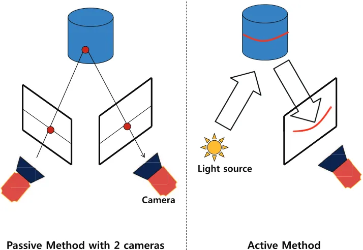
Figure 1.8: Basic principle of the active method.

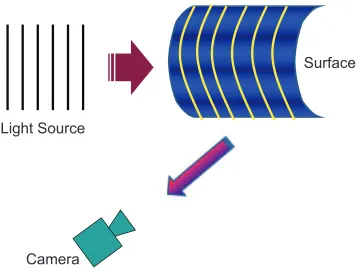
The proposed active approach consists of two viewpoints, one camera to capture a reflected image and one structured light source (Fig. 1.8). The light source generates structured circular patterns whose projected patterns onto an object, are captured as a 2D image. If the object is not a plane, the projected light patterns are deformed by the object shape. A camera acquires the deformed light patterns, and this deformation information of designed light patterns are geometrically related to the 3D coordinates of the object. This section presents some other examples of light patterns used to solve the reconstruction problem. The first one is a stripe pattern deformed by a surface shape (Fig. 1.9). Let a 3D point on the object illuminated by a stripe pattern, and a corre-sponding captured 2D image point be Mw = (Xw, Yw, Zw) and m = (u, v), respectively.

The projected stripe pattern defines a plane which is represented as

AXw +BYw+CZw+D= 0. (1.26)

(36)

Light Source

Camera

Surface

Figure 1.9: Active method using stripe patterns.

reconstruction problem (Fig. 1.10) [109]. Once the object coordinate system is aligned with the camera coordinate system, and we know Xw and Yw, the deformed pattern

provides a depth information of the object. Given the equation of a plane (Eq. (1.26)), and the assumption of a pinhole camera model, we have the following :

Xw =Zw

u

f, Yw =Zw v

f, (1.27)

AZw

u

f +BZw v

f +CZw+D= 0, (1.28)

Au f +B

v

f +C+ D Zw

= 0, (1.29)

Zw = −

Df

Au+Bv+Cf. (1.30)

(37)

Camera Camera Camera

Laser Laser

Object

Light Plane

0

w w w

Ax

By

Cz

D

_!

( , )

u v

Image Point

Figure 1.10: An example of a 3D reconstruction using stripe patterns [109].

method. When using an active method, the data acquisition from the deformed patterns is the most important step. Denoting the center of a light source and the optical center by S and C, respectively, geometrical relationship, as shown in Fig. 1.11 [37], can be represented as

sinθ

R =

sin(π₋α₋θ)

B , (1.31)

(38)

Figure 1.11: A geometrical relationship is a basic principle for a 3D reconstruction task in an active imaging [37]. B : Distance between center point of a light source and the optical center. R : Distance between the optical center and an object point.

Whichone?

1 0

t=1

t=2

t=3

(39)

Figure 1.13: To improve efficiency of coded structured light patterns, more complex patterns, such as gray-level or color coded patterns are employed [109].

efficient way is to assign more complicated codes to stripe patterns, for instance, gray-level or color coded light patterns (Fig. 1.13) [109]. When the structured light patterns are used for 3D reconstruction tasks, the phase being a property of light, may be used (Fig. 1.14). An observed image in a 2D image plane is composed of light intensities with phase information,

I1(x, y) = I0(x, y) +I(x, y) cos(φ(x, y)−θ),

I2(x, y) = I0(x, y) +I(x, y) cos(φ(x, y)),

I3(x, y) = I0(x, y) +I(x, y) cos(φ(x, y) +θ), (1.32)

whereφ(x, y) andθare a phase and a phase shift angle, respectively. Since φis a modulo of 2π, φ is written as

(40)

(41)

4GHGTGPEG2NCPG

_G

K

]

3 E

2CVVGTP2TQLGEVQT

QT.KIJV5QWTEG QT+OCIG5GPUQT%COGTC

1$,'%6

2TQLGEVKQP _4GHNGEVKQP

Figure 1.15: Example of a an experimental setup for 3D measurement using a structured light system [37].

and φ is represented using θ, I1,I2 and I3 [37],

φ′ _{= arctan}

"

tan(θ) I1−I3 2I2−I1−I3

#

. (1.34)

Given the information above, depth recovery is performed as follows (Fig. 1.15)

z = h−z

b d, (1.35)

z _∝ h

(42)

Figure 1.16: Example of a hybrid version of a combination of phase shift and coded light patterns [37].

Other active methods for reconstruction use a hybrid version consisting of a combination of phase shift and coded patterns (Fig. 1.16) [12], shadow patterns (Fig. 1.17) [118], De Brujin sequence patterns, etc. [37]. 3D reconstruction techniques based on structured light patterns are very widely used in many practical applications, e.g., facial imaging, medical imaging, reverse engineering, vehicle engineering, etc.

1.5 Sampling Theorem

Previous work in 3D reconstruction has focused on the accuracy of the reconstruction results. The optimal sampling density, or also referred to as the minimum sampling rate has not received much attention in the areas of 3D or high-dimensional signal recon-struction. There have, however, been many research activities to develop an adaptive sampling theorem beyond the Sahnnon-Nyquist Sampling Theorem in the areas of 1D signal processing [78]. The sampling theorem for 3D object is an open challenging topic and contributes a very important and core part of our contribution in this dissertation. (Chapter 4).

(43)

Figure 1.17: Simple 3D measurement using shadows [118].

will refer tof andf′ _as_f₍_t_{) and} _f₍_n_{) or}_f₍_nT_{), respectively. It has been almost 60 years}

since Shannon’s sampling theorem has been proposed, and it remains fundamental as it is widely used in many application calling for digital processing of signals. Discretization (sampling) and reconstruction procedures can be analytically written as

f(n) = X

n∈Z

f(t)δ(t−kT), (1.37)

f(t) = X

n∈Z

f(n)δ(t₋n). (1.38)

In some cases,δ(·) can be replaced byψ1 andψ2 which represent dual bases functions to determine f(n) and f(t), respectively if ψ1(t) and ψ2(t) satisfy the following :

1. Both ψ1 and ψ2 are orthogonal.

2. Both ψ1 and ψ2 are bandlimited.

(44)

minimum sampling rate lower than theNyquist Rate ([4, 27, 40, 96]). To achieve a more efficient sampling rate and to provide signal recovery from the sample set, an appropriate basis function ψ3(_·) is selected,

f(t) =X

n∈Z

f(n)ψ3(t₋Tn), (1.39)

where the interval Tn is not always uniformly distributed. In spite of various claims to

a sampling theorem beyond the Shannon-Nyquist Sampling Theorem, optimization pro-cesses for selecting basis function and irregular interval are always required a priori and highlight the complexity of adaptive sampling in a general setting. In Chapter 4, we pro-pose an approach to developing a sampling theorem to recover 3D objects represented by circular basis. The proposed method is in a sense a foundation for a sampling the-orem applied to 3D image processing, by establishing a relationship between frequency components and geometric information of a surface.

1.6 Interpolation Methods

Interpolation methods are often used in the areas of image processing for resampling [67] and improving a signal quality. Since the objective of interpolation is a reconstruction of a signal from a discrete signal or a sampled set of the signal, interpolation is closely related to sampling theorem. Nearest neighbor and linear interpolation methods were widely used techniques before the Shannon-Nyquist Sampling Theorem was introduced. In this section, we review some interpolation methods.

1. Nearest neighbor interpolation,

2. Linear interpolation,

3. Cubic interpolation,

(45)

When signal resampling is required, the interpolation process achieves a signal recon-struction from a subset of the signal. Following the Shannon-Nyquist Sampling theorem, the original signal is recovered by multiplication of an ideal sinc function whose Fourier transform is a rectangular function. In other words, since the inverse Fourier transform of the rectangular function is asinc function, the ideal interpolation can be a convolution with a sinc function. The ideal interpolator (Iideal(x)) in time domain can be written as

[67]

Iideal(x) =sinc(x) =

sin(πx)

πx (1.40)

However, an ideal sinc function is impossible to generate, and hence we can use other methods for interpolation, represented as a convolution withh(x), an approximated sinc function.

Nearest Neighbor Interpolation [53] Nearest Neighbor (NN) interpolation is one of

the simplest and widely used approaches. To reconstruct a signal, we assign the value at each position by taking the value of the nearest sampling point. But large errors due to a piecewise constant values, aliasing and blurring effect are drawbacks which are associated with NN interpolation method.

Linear Interpolation [26] In linear interpolation,sincfunction is approximately

rep-resented by triangular function.

h(x) =

(

1_{− |}x_|, 0_{≤ |}x_|<1

0, otherwise (1.41)

Another representation of the linear interpolation method is that a valuef(k) is estimated from the value at k₋1 and k+ 1 as follows

f(k) = 0.5f(k₋1) + 0.5f(k+ 1). (1.42)

Cubic Interpolation [62] Using algebraic polynomials to approximately represent the

(46)

be approximated by cubic polynomials. In cubic interpolation, h(x) is represented as

h(x) =

(

A_|x_|3₊_B_|_x_|2₊_C_|_x_|₊_D, ₀_{≤ |}_x_|_<₁

0, otherwise (1.43)

where A, B, C and D are determined using the boundary conditions [35].

Quadratic Interpolation [26] Similar to cubic interpolation, quadratic interpolation

methods also use algebraic polynomials to approximately represent an idealsincfunction. In quadratic interpolation, h(x) can be represented as

h(x) =

    

A_|x_|2₊_B_|_x_|₊_C, ₀_{≤ |}_x_|_<₁_/₂

D_|x_|2₊_E_|_x_|₊_F, ₁_/₂_{≤ |}_x_|_<₃_/₂

0, otherwise

(1.44)

with A, B, C,D,E, F ∈R_.

1.7 System Identification

(47)

information. In other words, this contribution is chiefly centered around approximate 3D reconstruction sufficient to characterize / classify a target object rather than a perfect 3D reconstruction. To that end, we develop an efficient 3D system identification frameworks based around an efficient 3D camera system as discussed in Chapter 7.

3D measurement from 2D information is conducted using structured light system. Any type of light patterns can be used and our reconstruction is on the basis of concentric circular patterns. In MPV system, to achieve an efficient reconstruction system, the optimal number and locations of cameras and projectors are investigated (Chapter 6). As previously mentioned, two alternative approaches are adopted, one ratio of input to output the other based on the modulation-demodulation theory.

(48)

System

Input

Output

x(t)

y(t)

Figure 1.18: A system (generally, static or dynamic) with input x(t) and outputy(t) is defined as the ratio of the output to input in frequency, Laplace or Z domain.

Transform and Z-Transform are widely used transformations for system identification,

Fourier Transform :

F(ω) =

Z +∞ −∞

f(t)e−jωtdt, (1.45) Laplace Transform :

F(s) =

Z +∞

0

f(t)e−stdt, (1.46)

Z- Transform :

F(z) = +∞

X

−∞

f[n]z−n, (1.47)

where f(t) is a signal, ω is a radial frequency, the parameter s = σ+jω is a complex number, and f[n] is a discretized signal of f(t),

f(nT) =f[n] =X

n∈Z

f(t)δ(t₋nT). (1.48)

(49)

iden-Input(s) or (Transmitted

Signal(s))

Output(s) or (Received Signal(s))

Estimated Input(s) modulation demodulation

cos( t) cos( t)

Figure 1.19: In communication theory, the modulation-demodulation theory is used to estimate the user(s) or transmitted signals from the output signal(s) using carrier signal, cosωt.

tification method, a 3D object is defined as the system, and we select an circular input signal rather than the ideal signals. The relevant information can be expressed as the ra-tio of output to input, where the output includes the informara-tion of captured images of the object overlaid with the light patterns, and the input includes the information of the original patterns projected onto the target. Instead of using ideal input signals, a single circular pattern is projected and the deformed pattern is captured on a 2D image plane. By monitoring the outputs (deformed patterns) corresponding inputs (original patterns), the system function is determined.

1.8 Modulation-Demodulation Theory

In communication systems, modulation-demodulation theory [81] is used to detect / estimate a transmitted signal (input signal). A carrier frequency is used for modulation and demodulation processes (Fig. 7.2). As illustrated in Fig. 7.2, a transmitted signal is estimated from the received signal by multiplying cosωt, where ω is a carrier frequency. Consider x(t) as a bandlimited signal whose bandwith is ωB. Let x(t) and y(t) be the

transmitted and received signals, the modulation can be written as

(50)

where ωc is a carrier frequency and we assume ωc >> ωB. The Fourier transform of y(t)

is carried out to simply analyze signals in the frequency domain.

Y(ω) = X(ω₋ωc) +X(ω+ωc), (1.50)

where X(ω) and Y(ω) are Fourier transform of x(t) and y(t) respectively. The demodu-lation is performed by multiplying y(t) by cosωct expressed as

Z(ω) =Y(ω₋ωc) +Y(ω+ωc), (1.51)

where Z(ω) is the demodulated signal of Y(ω), z(t) =y(t) cosωct, and rewritten as

Z(ω) = X(ω₋2ωc) +X(ω) +X(ω) +X(ω+ 2ωc). (1.52)

To complete the estimation of the transmitted signal, we need to retain the components containing ω. By using an ideal low-pass filter, 2ωc can be filtered out and 2x(t) is

(51)

1.8.1 Multiple View Geometry

In practice, a target object may be larger and can not be covered by a single camera and a projector. Structured circular light patterns may be generated by multiple light sources, and multiple cameras may capture the reflected deformed circular patterns. In the previous work, 3D reconstruction based on multiple view geometry has also con-centrated on the reconstruction accuracy, but our work emphasizes the efficiency of a multiple view reconstruction system in addition to the multiple projection system. We show that these are closely related to the geometric information of an object, and with minimal prior information, an efficient multiple-viewpoint-projector (MPV) 3D system is achieved (Chapter 6). Since objects of any size may be of interest, several projectors and cameras are required to solve the reconstruction problem, and the number of projectors and cameras need not be the same. The MPV system is a very useful approach to 3D reconstruction work using structured light systems. To achieve an efficient MPV system, the following require consideration,

(1) Orientations / locations of viewpoints and light sources,

(2) The number of viewpoints and light sources,

(3) The number of structured light patterns (sampling density),

(52)

This problem has also been addressed in [89], and it was shown that normal vectors of a surface are closely related to the determination of sensor planning. To achieve a successful illumination, our research shows that curvatures can determine the locations and the orientations of the projectors. When the object is illuminated by multiple light sources, overlapped light patterns are captured, and the reconstruction process based on the captured light patterns may be repeated in these areas. We assume that the object is only illuminated by projected light sources, and do not consider ambient light and light divergence here. In this environment, overlapped light patterns have different intensity values from the areas illuminated by a single light source, and the intensity variation is a key to detecting overlapped regions. Detecting the overlapped areas contribute to the reconstruction efficiency by avoiding redundancy and repeated reconstruction. The location, the orientation and the number of cameras are related to the distance between neighboring cameras. The minimum number of cameras to capture the target object is required to increase a system efficiency. This contribution is detailed in Chapter 6.

1.9 Classification for Recognition

If the ground truth model is not provided, the performance evaluation of the recon-struction is difficult to asses. To that end we use an approximate reconrecon-struction result which is sufficient to identify a target, to recognize / classify a target. Comparing circu-lar pattern based representations of two objects is one way of carrying out identification, classification and recognition, and the resulting performance is subsequently used as a reconstruction performance measure. In light of large data set of 3D objects, it is par-ticularly important to utilize efficient representations of objects. Principal component analysis (PCA) [100] is one of the classical and widely used data reduction methods. The PCA method for eigenfaces, for instance, eigenvectors of the signal / data covari-ance matrix, is used to represent the properties of object information (usually M by

(53)

the literature. PCA, however, presents limitations when nonlinear structures are present in the data. The limitations require nonlinear mapping approaches such as Kernel PCA (KPCA), Local Linear Embeddinig (LLE), Self Organizing Map (SOM), etc. The basic principle of nonlinear methods is applying a functional to the original datasets X.

Y= Φ(X), (1.53)

where Φ(·) maps the original dataX to the lower dimensional space [86]. LLE is another widely used nonlinear approach to dimensionality reduction. The LLE algorithm uses neighboring data points followed by estimating a weight factor matrix W which can most accurately represent (or reconstruct) a data point as its neighboring points.

E(W) = X

i

|Xi−

X

j

WijXj|2, (1.54)

where Wij is selected to minimize the cost function E(W). The dataX is then mapped

toY which is in the lower dimensional space (X and Y are any dimensional vectors and

W is a matrix composed of elements [W]ij). Each component of Y is represented by

using the weight factors estimated above and Y is composed of Yi which minimizes the

embedding cost function Φ(Y) ([82, 85]).

Φ(Y) = X

i

|Yi−

X

j

WijYj|2, (1.55)

Similar to PCA, Locality Preserving Projection (LPP), Orthogonal LPP (OLPP) also project the original data to the lower dimensional space. LPP uses the same approaches as PCA, but it assigns a weight factor to the object function according to connectivity between all pairs of data points. OLPP is an extended version of OPP which adds the constraint of orthogonality to the projection matrix P (i.e. PPT ₌ _I_{) The approaches}

(54)

points of the data set lying in the higher dimensional manifold. Geodesic or Euclidean distance between data points on a surface can represent intrinsic geometric properties of the object, and these approaches are categorized as multi dimensional scaling (MDS). Some examples of MDS are ISOMAP and curvilinear component analysis (CCA). They use the distance between all pairs of data points and achieve a lower dimensional object representation which best preserves the intrinsic geometric structure of a target object. In addition, there have been many proposed algorithms for dimensionality reduction [9] and several robustness and drawbacks of existing nonlinear dimensionality reduction methods have been addressed in ([52, 60, 121]).

Dimensionality reduction is clearly important in data processing and can be applied to image processing particularly in a recognition / classification applications. The proposed the dimensionality reduction approach, in the sequel is for efficient object classification for a recognition system.To achieve reliable recognition or classification results (e.g. ac-ceptance rate), many algorithms have been proposed, for instance, 2D or 3D based, 2D + 3D based, feature based, geometry based approaches [5, 10, 33, 75, 84].

This work herein proposes an approach to face classification and recognition using di-mensionality reduction based on deformed circular curves, the shortest geodesic distances and the properties of the Fourier Transform. The original signal (of 3×M ×N size) is represented as a 0.5×M ×N size signal, preserving the characteristics of the original signal. To achieve dimensionality reduction, a geodesic distance between the reference point and a point on the surface is measured. Note that the geodesic distance preserves the intrinsic property of a 3D object. By measuring the geodesic distance between the reference point and a point on the curve, data size is reduced toM_×N. Once theM_×N

(55)

1.10 Organization and Contributions

(56)

Chapter 2 3D Reconstruction from 2D Image

2.1 Introduction

(57)

problem is solved by establishing a relationship between the different points of the same object, the reconstruction result highly depends on the points in 2D image planes. In addition, the limitation of the passive method is that tremendous elaboration is required to acquire sufficient 2D data points from 2D image planes. The alternative approach to the reconstruction problem is an active stereo vision, or an active method, using a structured light system which has attracted tremendous interests [80]. In active method, one camera is replaced by an active light source such as an LED or a laser beam that projects a known pattern. Only one camera is used to capture the projected pattern on a 3D object to be measured. Structured light patterns with high resolution can achieve a large number of sampling points over the surface and result in high reconstruction accuracy [59]. In this chapter, we assume that the position of a camera and a light source are known, a camera is modeled as an ideal camera (often called a pinhole model) and the light projection is parallel [76] (Fig. 2.6). In practice, however, a camera is not usu-ally calibrated to a pinhole model and structured patterns do not exactly preserve their shape by a set of lenses (lens distortion), but it is very difficult to model the system [8]. The observed deformation of the projected pattern on a 3D object provides information of its real world 3D coordinates (xw, yw, zw) by establishing a relationship between the

(58)

d d Projection

d1 d2

1 2

d

Figure 2.1: Ideal and deformed circles.

Section 2.3, containing the major contribution of this paper, presents notations for image representation (Section 2.3.1) and details the proposed mathematical model to achieve the reconstruction procedure (Section 2.3.2). Some preliminary experimental results are shown in Section 7.5 to substantiate the mathematical model proved in Section 2.3.2. Finally, Section 2.5 summarizes the chapter and proposes future works. Parts of this chapter have appeared in [64].

2.2 System Architecture

2.2.1 Overall System Description

(59)

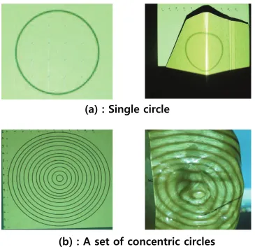
C5KPINGEKTENG

D#UGVQHEQPEGPVTKEEKTENGU

Figure 2.2: Ideal and projected(observed) circular patterns.

geometrical relationships between 2D acquired data and real world 3D coordinates, and a reconstruction (Fig. 2.4). Prior to projection of light patterns, in practice, calibration process for a camera is required for an accurate reconstruction, but we assume that the camera is already calibrated and chiefly deals with the proof of concepts to develop a mathematical model to solve the reconstruction problem.

(60)

Figure 2.3: Setup of structured light projection system using LC2002.

Circular Pattern Projection

2D Data Acquisition

Geometrical

Analysis Reconstruction

(61)

positions.

2.3 Surface Reconstruction

2.3.1 Notations and Geometrical Representation

Let S _⊂ R3 _{be a domain of a 3D object of interest, then a point on the object surface} Pw ∈S is represented as

Pw = {(xw, yw, zw)∈R3}, (2.1)

where an index w is used to denote real world coordinates. Let L⊂ R3 _{be a domain of}

a circular structured light source and the origin defined as a center of a pattern (or a curve), then a point PL ∈Lis represented as

PL = {(xLij, yLij, zLij)∈R3 | x2Lij+yLij2 =R2j, zLij = 0},

i = 1,2, . . . , M, j = 1,2, . . . , N, (2.2)

where we set zLij = 0 an arbitrary reference plane of the light source space. Let S3 ∈R3 be a domain of projected circular patterns projected onto a 3D object, then P3 ⊂ S3 is represented as

P3 = {(xwij, ywij, zwij)∈R3}, (2.3)

i = 1,2, . . . , M, j = 1,2, . . . , N.

After the patterns projected, P3 and Pw defined in the intersection of S and S3 are identical,

(62)

L

S₃

S₂

P_L

P₃

P2

X Y

-Z

Light Source

Object

Camera (Image Plane)

Figure 2.5: Geometrical representation of domains of the light source, 3D surface and 2D image plane.

Let S2 ⊂ R2 be a domain of 2D image plane of a camera (or observation space), then

P2 ∈S2 is represented as

P2 = {(uij, vij)∈R2}, i= 1,2, . . . , M, j = 1,2, . . . , N, (2.5)

where N is a number of projected patterns and M is a number of sampled points in each pattern. We assume that M is sufficiently large and N can be optimized for sys-tem efficiency which leads to the motivation for developing a sampling theorem which determines the minimum number of light patterns (Nmin) for the reconstruction. The 3D

An Efficient 3D Imaging using Structured Light Systems.

ABSTRACT

DEDICATION

BIOGRAPHY

ACKNOWLEDGEMENTS

TABLE OF CONTENTS

LIST OF TABLES

LIST OF FIGURES

Chapter 1

Introduction

1.1

Projective Geometry

Retinar plane

C : Optical center

M

: Real world position

m : point in an image

1.2

Camera Calibration

1.2.1

Extrinsic Parameters

1.2.2

Intrinsic Parameters

X

X

Y

P

P

Y

1.3

3D Reconstruction - Passive Stereo Vision

M

Z

Y

Z

u

v

c

m

f

C

m’

C’

C

C’

M

e

e

m

m’

Object

%

&DPHUD

1.4

3D Reconstruction - Active Stereo Vision

Light Source

Camera

Surface

0

Ax

By

Cz

D

!

( , )

u v

4GHGTGPEG2NCPG

G

K

]

3

E

1$,'%6

1.5

Sampling Theorem

1.6

Interpolation Methods

1.7

System Identification

System

_!

_G