Efficient uncertainty quantification for biotransport in tumors with uncertain material properties

EFFICIENT UNCERTAINTY QUANTIFICATION FOR BIOTRANSPORT IN TUMORS

WITH UNCERTAIN MATERIAL PROPERTIES

Alen Alexanderian Department of Mathematics

Center for Research in Scientific Computation North Carolina State University

Raleigh, NC 27695 Email: [email protected]

William Reese Department of Mathematics North Carolina State University

Raleigh, NC 27695

Ralph C. Smith Department of Mathematics

Center for Research in Scientific Computation North Carolina State University

Raleigh, NC 27695

Meilin Yu∗

Department of Mechanical Engineering University of Maryland, Baltimore County

Baltimore, MD 21250 Email: [email protected]

ABSTRACT

We consider modeling of single phase fluid flow in hetero-geneous porous media governed by elliptic partial differential equations (PDEs) with random field coefficients. Our target ap-plication is biotransport in tumors with uncertain heterogeneous material properties. We numerically explore dimension reduc-tion of the input parameter and model output. In the present work, the permeability field is modeled as a log-Gaussian ran-dom field, and its covariance function is specified. Uncertain-ties in permeability are then propagated into the pressure field through the elliptic PDE governing porous media flow. The covariance matrix of pressure is constructed via Monte Carlo sampling. The truncated Karhunen–Lo`eve (KL) expansion tech-nique is used to decompose the log-permeability field, as well as the random pressure field resulting from random permeabil-ity. We find that although very high-dimensional representation is needed to recover the permeability field when the correlation length is small, the pressure field is not sensitive to high-oder KL terms of input parameter, and itself can be modeled using a low-dimensional model. Thus a low-rank representation of the

pres-∗_{Address all correspondence to this author.}

sure field in a low-dimensional parameter space is constructed using the truncated KL expansion technique.

INTRODUCTION

Understanding biotransport processes in tumors with uncer-tain material properties is important for agent (e.g., drug, nano-particles) delivery in cancer treatment [1, 2]. Biotransport pro-cesses in tumors can be modeled as flows in porous media, with random heterogeneous material properties, governed by different types of PDEs: an elliptic PDE, which describes the pressure dis-tribution; and a hyperbolic PDE, which describes agent delivery in porous media [3]. Therefore, uncertainties in the PDE coef-ficient fields will be propagated into the flow field via complex fluid and tumor structure interaction described by these PDEs [4]. In this work, we focus on elliptic PDEs, modeling single phase fluid flow in heterogeneous porous media. The permeability field is modeled as a log-Gaussian random field, and the goal is to ef-ficiently simulate the uncertain pressure field. The random per-meability field is represented through its KL expansion [5].

with enough terms to ensure a sufficiently accurate representa-tion. This truncated KL expansion, which is computed upfront, is then substituted in the governing PDEs, after which appropri-ate uncertainty analysis is performed. The study presented herein takes a different point of view: instead of relying on a truncated KL expansion of the parameter, computed a priori and indepen-dently of the governing PDE, we argue that only the KL terms that the PDE solution operator is sensitive to should be retained. Moreover, we explore the KL expansion of the PDE solution, for computing a low-rank representation of the model output.

In presence of small correlation lengths, a large number of terms in the KL expansion are required to represent the uncertain permeability field. However, it is observed that, for the pres-sure equation, the PDE solution operator is not sensitive to the high-order KL terms of the parameter. This enables reducing the dimension of the input parameter, by focusing on the KL terms that are most influential to variations in the pressure field. The PDE solution—the pressure field—itself can also be repre-sented via a truncated KL expansion. It is again observed that a low-rank representation of the pressure field is often afforded by a suitably truncated KL expansion. Combining these ideas enables a rank representation of the pressure field in a low-dimensional parameter space. We first illustrate these ideas using a one-dimensional (1D) model elliptic PDE, and then further ex-plore the proposed approach in a two-dimensional (2D) model of biotransport in a tumor with uncertain material properties.

BACKGROUND ON RANDOM FIELDS

We let(Ω,F,P)be a probability space, whereΩis a

sam-ple space,F is an appropriateσ-algebra, andPis a probability

measure. LetD⊂_Rd_{, withd=1,2, or 3, be a d-dimensional}

bounded physical domain. We consider stochastic processes of

formZ:D×Ω→R; for background material on stochastic

pro-cesses, we refer the reader to [16]. From a practical point of

view, Z(x,ω)can be used to model uncertain field parameters

appearing in PDEs governing the physical systems.

We call a stochastic processcentered if E[Z(x,·)] =0 for

all x∈D, where E[·] denotes mathematical expectation, i.e., E[Z(x,·)] =R

ΩZ(x,ω)P(dω). A processZ is said to bemean

square continuousif for allx∈D,

lim

h→0E[(Z(x+h,·)−Z(x,·))

2_{] =0.}

Karhunen–Lo`eve expansion. The covariance functionc:

D×D→_Rof a stochastic processZis defined as

c(x,y) =E[Z(x,·)Z(y,·)]−E[Z(x,·)]E[Z(y,·)], (1)

and the corresponding correlation function is given by,

ρ(x,y) =_p c(x,y)

c(x,x)pc(y,y).

Given the covariance function ofZ(x,ω), the associated

covari-ance operator C:L2(D)→L2(D)is defined as

[Cu](x) =

Z

D

c(x,y)u(y)dy, (2)

whereL2(D) ={f:D→R:RD|f(x)|2dx<∞}.

LetZ :D×Ω→Rbe a centered mean-square continuous

stochastic process, and let{ei}∞i=1 be the orthonormal basis of

eigenvectors of the covariance operatorCofZ(x,ω)with

corre-sponding (non-negative) eigenvalues{λi}∞i=1:

Z

D

c(·,y)ei(y)dy=λiei(·), i=1,2, . . . . (3)

The processZ(x,ω)can be represented as

Z(x,ω) = ∞

∑

i=1

p

λiξi(ω)ei(x), (4)

where ξi are centered mutually uncorrelated random variables

with unit variance and are given by,

ξi(ω) =

1

√

λi

Z

D

Z(x,ω)ei(x)dx.

The convergence of the series (4) is uniform inD, and is mean

square inΩ [5]. The series expansion (4) is known as the KL

expansion [5, 17–19] ofZ(x,ω).

Numerical computation of KL expansion. Here we

out-line a basic approach for computing the KL expansion of a stochastic process (random field). To numerically compute the KL expansion of a stochastic process we need to first solve

the eigenvalue problem (3). Here, we follow Nystr¨om’s

ap-proach [20], in which the generalized eigenvalue problem is dis-cretized via quadrature. In some cases, one can specify the co-variance function of the process via an analytic formula. This is the case, for instance, when modeling uncertain coefficient fields in mathematical models via Gaussian processes, as seen later in the present work. On the other hand, in some cases, we only can simulate realizations of a given stochastic process. The latter is the case, when working with solution of a PDE with uncertain

often one parameterizes model uncertainties via a random vector

ξξξ(ω), in which case the random field solutionU=U(x,ξξξ)of the

PDE can be computed for specific realizations ofξξξ. To compute

the truncated KL expansion,

U(x,ξξξ)≈_U(¯ _{x) +}

Nkl

∑

i=1

p

λiui(ξξξ)ei(x),

¯

U(x) =E[U(x,·)],

ui(ξξξ) =√1 λi

Z

D

(U(x,ξξξ)−U(¯ x))ei(x)dx,

(5)

the covariance function of the process needs to be approximated via sampling; this in turn leads to an approximate covariance

op-eratorC for the process. The approximate covariance operator

is then used to formulate and solve the generalized eigenvalue problem to find (approximations to)λiandei,i=1, . . . ,Nkl. In

Algorithm 1, we summarize the process of computing the

trun-cated KL expansion of a random processU(x,ξξξ)by sampling

its covariance function. In the sequel, we call the coefficientsui

in (5) theKL modes. For further details on numerical techniques

for computing KL expansions, we refer to [21].

MODEL 1D ELLIPTIC EQUATION WITH RANDOM CO-EFFICIENT FUNCTION

Let(Ω,F,P)be a probability space. We consider the

fol-lowing elliptic boundary value problem: forω∈Ω, find a

func-tionpsuch that

−d

dx

κ(x,ω)d p(x,ω)

dx

=f(x), x∈D= (−1,1),

p(−1,ω) =1,

p(1,ω) =0.

(6)

In the following numerical experiments, the right hand side

func-tion is given by f(x) =cos(πx) +sin(2πx). We model the

coef-ficient function κ(x,ω) as a log-Gaussian random field in the

following manner. LetZ(x,ω)be a centered Gaussian process

with covariance function,

cZ(x,y) =exp

n

−|x−y|

`

o

. (7)

The number`≥0 is the correlation length of the process, which

in the present work is set to`=1/4; i.e., 12.5% of the length of

the domain. We defineκ(x,ω) =exp(a(x,ω))with

a(x,ω) =a0(x) +σZ(x,ω). (8)

Hereσ2is the pointwise variance anda0is the pointwise mean;

these parameters are chosen to obtain a pointwise mean ofm=

0.1 and pointwise standard deviation ofs=.07 forκ(x,ω): we

letσ2=log(1+s2/m2)anda0≡log m/p1+s2_/m2

.1 To facilitate computations, we consider a truncated KL ex-pansion ofZ(x,ω); thus, we use

a_Na

kl(x,ω) =a0+σ

Na kl

∑

i=1

p

λiξi(ω)ei(x), (9)

where (λi,ei) are eigenpairs of the covariance operator of

Z(x,ω). Due to Gaussianity of the process,ξi are independent

standard normal random variables. The random vector

ξ ξ

ξ =ξ1ξ2· · · ξN_kla

T

(10)

completely characterizes the uncertainty in the PDE (6), and its solutionp(x,ω) =p(x,ξξξ(ω)).

The eigenpairs of the covarince operator [CZu](x) =

R

DcZ(x,y)u(y)dyare computed numerically by discretizing the

corresponding generalized eigenvalue problem, as explained in the previous section. The truncation of the KL expansion of

Z(x,ω)is guided by considering the ratio,

r(N) =∑

N i=1λi

∑∞i=1λi

, (11)

which quantifies the percentage of the average variance captured

by the firstNKL terms.

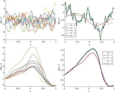
Realizations of a(x,ω) and the corresponding

realiza-tions of p(x,ω). Using the truncated KL expansion in (9), we

can approximate the log-coefficient field efficiently. The top-left

image in Figure 1 shows several realizations of a(x,ω),

corre-sponding toNa

kl=70. The corresponding solutions of the

prob-lem (6) are reported in Figure 1 (bottom-left). To demonstrate the impact of changing the number of KL terms on the realiza-tions ofa(x,ω), we consider a fixed realization ofa(x,ω)asN_kla

increases. We note in Figure 1 (top-right) that for the present pro-cess with the specific choice of correlation structure, sufficiently largeN_kla is needed to capture the fluctuations of the random field reasonably well. On the other hand, the PDE solution seems in-sensitive to the higher-order KL terms of the parameter, as seen in Figure 1 (bottom-right). This suggests that it is possible to re-duce parameter dimension by retaining only the terms in the KL expansion (9) that have notable impact on PDE solution.

1_{Here we use the well-known formulas relating the mean and variance of a}

log-normal random variableY=exp(a0+σX), whereXis standard normal, to

Algorithm 1Computing KL expansion of a random processU(x,ξξξ)using Nystr¨om’s approach.

Input: (i) A quadrature formula onDwith nodes and weights{xm,wm}

Nquad

m=1; (ii) function evaluations{U(xm,ξξξk)},m∈ {1, . . . ,Nquad}, k∈ {1, . . . ,N}; (iii) trunction levelNkl.

Output: Eigenpairs of the discretized covariace operator,{(λi,ei)}iN=kl1, and KL modes{ui}Ni=kl1.

1: Compute the mean

¯ Um=

1 N

N

∑

j=1

U(xm,ξξξj), m∈ {1, . . . ,Nquad}.

2: Center the process

uc(xm,ξξξk) =U(xm,ξξξk)−U¯m, k∈ {1, . . . ,N},m∈ {1, . . . ,Nquad}.

3: Form the covariance matrix

Klm=

1 N−1

N

∑

k=1

uc(xl,ξξξk)uc(xm,ξξξk), l,m∈ {1, . . . ,Nquad}.

4: LetW=diag(w1,w2, . . . ,wNquad)and solve the eigenvalue problem

W1/2KW1/2vi=λivi, i∈ {1, . . . ,Nquad}.

5: Computeei=W−1/2vi,i∈ {1, . . . ,Nquad}.

6: Compute the discretized KL modes,

ui(ξξξk) =√1 λi

Nquad

∑

m=1

wmuc(xm,ξξξk)e_im, i∈ {1, . . . ,Nkl},k∈ {1, . . . ,N}.

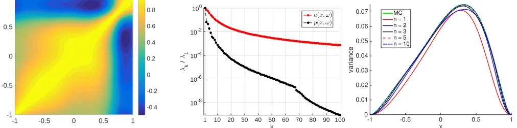
Spectral representation of p(x,ω). In this section, we

study the approximation of the PDE solutionp(x,ω)using

trun-cated KL expansions computed using Algorithm 1. We begin

by depicting the correlation function ofp(x,ω)in Figure 2 (left)

approximated via Monte Carlo sampling with 104_{samples; this}

illustrates the long correlation lengths observed in the solution of the uncertain boundary value problem. Hence, we expect that

the eigenvalues of the covariance operator ofp(x,ω)will exhibit

faster decay as compared to eigenvalues ofCZ. This

observa-tion is shown to be the case in Figure 2 (middle) where we com-pare the (normalized) eigenvalues of the covariance operators for p(x,ω)anda(x,ω). This suggests that p(x,ω)can be

approxi-mated well with a truncated KL expansion with a small number

of terms. Hence, we consider the KL expansion

p(x,ω) =p(x) +¯ ∞

∑

j=1

√

µjpj(ω)vj(x). (12)

ofp(x,ω), whereµj,vjare the eigenpairs of covariance operator

of p, computed numerically,pjare given by

pj(ω) =√1 µj

Z

D

(p(x,ω)−p(x))v¯ j(x)dx, j=1,2, . . . ,

and ¯p(x)is the mean ofp(x,ω). One way to quantify the impact

of truncating the KL expansion of p(x,ω)on its approximation

-1 -0.5 0 0.5 1 x

-5 -4 -3 -2 -1 0

a(x,

ω

)

-1 -0.5 0 0.5 1

x

-3.5 -3 -2.5 -2 -1.5

a(x,

ω

)

Na KL = 2 Na

KL = 4 Na_KL = 10 Na

KL = 30 Na

KL = 70

-1 -0.5 0 0.5 1

x 0

1 2 3 4 5 6

p(x,

ω

)

-1 -0.5 0 0.5 1

x 0

0.5 1 1.5 2 2.5 3 3.5

p(x,

ω

)

Na KL = 2 Na

KL = 4 Na

KL = 10 Na

KL = 30 Na

KL = 70

FIGURE 1. Top row: Several realizations of the log-coefficient field withN_KLa =70 (left); and a fixed realization of the log-coefficient field as we increaseN_KLa (right). Bottom row: Solutions of the problem (6) corresponding to the realizations of the log-permeability field plotted in the top-left image (left), and a fixed realization ofp(x,ω)as we increaseN_KLa (right).

different truncation levels. It is straightforward to see

Var





N_klp

∑

j=1

√

µjpj(ω)vj(x)



=

N_klp

∑

j=1

µjvj(x)2.

In Figure 2 (right), we see that it is possible to approximate the pointwise variance ofp(x,ω)well with a smallN_klp.

These numerical experiments lead to the following conclu-sions:

• It is possible to reduce parameter dimension by focusing on

KL terms of the parameter that the PDE solution operator is most sensitive to.

• It is possible to reduce output dimension by focusing on the

dominant KL terms of the output.

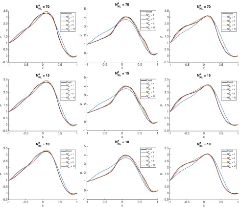
Based on these observation, we next examine parameter and out-put dimension reduction. In Figure 3 we depict typical

realiza-tions of p(x,ω), as the parameter and output dimension is

sys-tematically reduced. These results indicate that simultaneous pa-rameter and output dimension reduction is possible.

APPLICATION TO BIOTRANSPORT IN TUMORS

Governing equations and numerical setup.In this section,

we study the pressure field in a tumor when a single needle injec-tion occurs at the tumor center. A 2D model in a polar coordinate system is used to analyze the flow field. Consider the mass con-servation law and Darcy’s law for steady incompressible flows in a 2D domain,D={(r,θ):Rneedle<r<Rtumor,0<θ<2π},

∂

∂r

κr

µ ∂p

∂r

+1 r

∂

∂ θ

κ

µ ∂p

∂ θ

=0. (13)

Here p is the pressure,κ is the permeability,µ is the fluid

dy-namic viscosity,ris the radial distance from a fixed origin,θis

the polar angle,Rtumor is the radius of the tumor, andRneedleis

k

1 10 20 30 40 50 60 70 80 90 100

λk

/

λ1

10-8 10-6 10-4 10-2 100

a(x, ω) p(x, ω)

x

-1 -0.5 0 0.5 1

variance

0 0.01 0.02 0.03 0.04 0.05 0.06

0.07 MC

n = 1 n = 2 n = 3 n = 5 n = 10

FIGURE 2. Left: Correlation function; middle: decay of the spectrum ofa(x,ω)(red) versus that of the solutionp(x,ω)(black); we report the first

100 normalized eigenvalues with correlation length of 1/4 for the log-parameter fielda(x,ω). Right: pointwise variance ofp(x,ω), computed using

KL expansion of varying truncation levels, against pointwise variance computed using 10,000 Monte Carlo samples.

The boundary conditions for the pressure equation are spec-ified as follows:







p=0, r=Rtumor,

∂p

∂r

= −Qµ 2πRneedleκ

, r=Rneedle.

(14)

Herein, Q is the volume flow rate per unit length. Periodic

boundary conditions are enforced in theθdirection. In this study,

RneedleandRtumorare set to 0.25mmand 5mm, respectively. Here

Qis 0.2mm2/min, andµis 8.9×10−4Pa·s.

Uncertainties in permeability field. As before let

(Ω,F,P)be a probability space. Following [4], the permeability

κis modeled by a log-Gaussian random field, and its mode is set

to 0.5md, wheremdstands for millidarcy. We assume that the

log-permeability,a(x,ω) =log κ(x,ω)), is given by

a(x,ω) =a0(x) +σaZ(x,ω), x∈D,ω∈Ω.

Herea0is the pointwise mean of the process, σ_a2 is the

point-wise variance, andZ is a centered Gaussian process with unit

pointwise variance for everyx∈D. Herein, σ_a2 is set to 0.25,

and a0 is calculated from the definition of the mode of κ as

a0=ln(0.5) +σ_a2. The covariance function ofZ is expressed

as cZ(x,y) =exp−1<sub>`</sub>kx−yk2 , x,y∈D, where` >0 is the correlation length. The log-permeability field can be expressed with a truncated KL expansion:

a(x,ω)≈a0(x) +σa N_kla

∑

k=1

√

λkξk(ω)ek(x), (15)

whereλkandekare eigenpairs of the covariance operator of the

processZ. As before, due to Gaussianity of the process,ξk are

independent standard normal random variables.

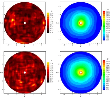
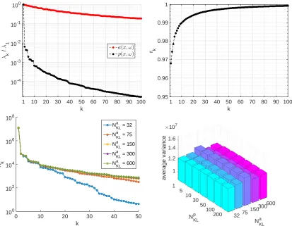
Whereas the governing equation is more complex than the previously considered 1D elliptic problem, it is still an elliptic PDE and hence we observe similar behavior in terms of potential for dimension reduction. Two sets of realizations of the perme-ability field and the corresponding pressure field, when a small

correlation length of`=0.5mmis used for the log-permeability

field, are presented in Figure 4. We observe that although there exist large fluctuations in the permeability field, the fluctuations in the pressure field are mild. For ease of exposition, we denote

the covariance operator of the log-permeability field byCa and

that of the pressure field byCp. The eigenvaluesλi(Cp)show a

far more rapid decay as compared to that ofCa, as seen in

Fig-ure 5 (top left). In FigFig-ure 5 (top right), we note that more than

96% of the average variance in pas computed by ∑ki=1λi(Cp),

is captured the first KL term and adding a few KL terms leads to capturing more than 99% of the power spectrum. The

eigen-values ofCpare approximated using Algorithm 1, with a Monte

Carlo sample of sizeN=5000. Next, we experiment with

si-multaneously changing N_kla andN_klp. This is done by

consider-ing KL expansions of the log-permeability field withN_kla terms,

sampling the resulting KL expansion, and computing p(x,ω)by

solving the pressure equation for each log-permeability field re-alization. These samples of the PDE solution are then passed to Algorithm 1 to compute the KL expansion of the pressure field. In Figure 5 (bottom left), we show λk(Cp),k=1, . . . ,50,

cor-responding to N_kla ∈ {32,75,150,300,600}. We note that even

withN_kla =32, we can approximate the first 10 eigenvalues of

Cp, which carry most of the power spectrum, reasonably well.

Finally, in Figure 5 (bottom right), we show the approximations

to average variance ofp(x,ω), computed by∑

N_klp

k=1λk(Cp), asN

a kl

andN_klp change. Again, we see that the average variance can be

x

-1 -0.5 0 0.5 1

p -0.5 0 0.5 1 1.5 2 2.5 3 3.5 N KL a = 70 Exact N_KLp _{= 1}

N_KLp _{= 3}

N_KLp = 5 N_KLp _{= 10}

x

-1 -0.5 0 0.5 1

p -1 0 1 2 3 4 5 N KL a = 70 Exact N KL p _{= 1}

N_KLp = 3 N_KLp _{= 5}

N

KL p _{= 10}

x

-1 -0.5 0 0.5 1

p -0.5 0 0.5 1 1.5 2 2.5 3 3.5 N KL a = 70 Exact N_KLp _{= 1}

N_KLp _{= 3}

N_KLp = 5 N_KLp _{= 10}

x

-1 -0.5 0 0.5 1

p -0.5 0 0.5 1 1.5 2 2.5 3 3.5 N KL a = 15 Exact N_KLp _{= 1}

N_KLp _{= 3}

N_KLp = 5 N_KLp _{= 10}

x

-1 -0.5 0 0.5 1

p -1 0 1 2 3 4 5 N KL a = 15 Exact N KL p _{= 1}

N_KLp = 3 N_KLp _{= 5}

N_KLp = 10

x

-1 -0.5 0 0.5 1

p -0.5 0 0.5 1 1.5 2 2.5 3 3.5 N KL a = 15 Exact N_KLp _{= 1}

N_KLp _{= 3}

N_KLp = 5 N_KLp _{= 10}

x

-1 -0.5 0 0.5 1

p -0.5 0 0.5 1 1.5 2 2.5 3 3.5 N KL a = 10 Exact N_KLp _{= 1}

N_KLp _{= 3}

N_KLp = 5 N_KLp _{= 10}

x

-1 -0.5 0 0.5 1

p -1 0 1 2 3 4 5 N KL a = 10 Exact N KL p _{= 1}

N_KLp _{= 3}

N_KLp _{= 5}

N_KLp = 10

x

-1 -0.5 0 0.5 1

p -0.5 0 0.5 1 1.5 2 2.5 3 3.5 N KL a = 10 Exact N_KLp _{= 1}

N_KLp _{= 3}

N_KLp = 5 N_KLp _{= 10}

FIGURE 3. Realizations ofp(x,ω)and the corresponding truncated KL expansions ofp; each row corresponds to approximations computed with

different truncation levels for the parameter, as indicated byNa

KLin figure titles.

CONCLUSIONS

We have studied the input parameter and output dimension reduction of elliptic PDEs, with random field input parameters, via the truncated KL expansion technique. In this study, the covariance function of the stochastic process defining the input parameter field is given, and that of the random output is con-structed via Monte Carlo sampling. From numerical experiments with both 1D and 2D elliptic PDEs, we observe that when the correlation length is small, very high-dimensional representation is needed to fully resolve the variations in the input field. How-ever, the elliptic operator is not sensitive to high-order KL terms.

FIGURE 4. Two sets of realizations of the permeability field (left) and the corresponding pressure field (right). The correlation length`is 0.5mm.

REFERENCES

[1] Salloum, M., Ma, R., Weeks, D., and Zhu, L., 2008. “Con-trolling nanoparticle delivery in magnetic nanoparticle hy-perthermia for cancer treatment: experimental study in

agarose gel”.Int. J. Hyperthermia, 24, pp. 337–345.

[2] Debbage, P., 2009. “Targeted drugs and nanomedicine:

present and future”. Current Pharmaceutical Design, 15,

pp. 153–72.

[3] Swartz, M. A., and Fleury, M. E., 2007. “Interstitial flow

and its effects in soft tissues”.Annu. Rev. Biomed. Eng., 9,

pp. 229–56.

[4] Alexanderian, A., Zhu, L., Salloum, M., Ma, R., and Yu, M., 2017. “Investigation of biotransport in a tumor with uncertain material properties using a non-intrusive spectral

uncertainty quantification method”.Journal of

Biomechan-ical Engineering, 139(9), p. 091006.

[5] Loeve, M., 1977. Probability theory I, Vol. 45 of

Gradu-ate Texts in Mathematics. New York, Heidelberg, Berlin: Springer-Verlag.

[6] Ghanem, R., 1998. “Probabilistic characterization of

trans-port in heterogeneous media”. Computer Methods in

Ap-plied Mechanics and Engineering, 158(3), pp. 199 – 220. [7] Le Maˆıtre, O. P., Reagan, M. T., Najm, H. N., Ghanem,

R. G., and Knio, O. M., 2002. “A stochastic projection

method for fluid flow: Ii. random process”.Journal of

com-putational Physics, 181(1), pp. 9–44.

[8] Xiu, D., and Karniadakis, G. E., 2003. “Modeling

un-certainty in flow simulations via generalized polynomial

chaos”.Journal of Computational Physics, 187(1), pp. 137

– 167.

[9] Le Maıtre, O., Knio, O., Najm, H., and Ghanem, R., 2004. “Uncertainty propagation using wiener–haar expansions”. Journal of computational Physics, 197(1), pp. 28–57. [10] Babuˇska, I., Nobile, F., and Tempone, R., 2007. “A

stochas-tic collocation method for ellipstochas-tic partial differential

equa-tions with random input data”.SIAM Journal on Numerical

Analysis, 45(3), pp. 1005–1034.

1 10 20 30 40 50 60 70 80 90 100 k

10-4 10-3 10-2 10-1 100

λ k

/

λ 1 a(x, ω)

p(x, ω)

1 10 20 30 40 50 60 70 80 90 100

k 0.95

0.96 0.97 0.98 0.99 1

r k

0 10 20 30 40 50

k 100

102 104 106 108

λ k

N KL a

= 32

N KL a

= 75

N KL a _{= 150}

N KL a

= 300

N KL a

= 600

FIGURE 5. Top: spectrum of the PDE solution vs spectrum of the uncertain parameter (left); the ratiork=∑ki=1λi/∑Ni=1λi, withN=200, showing

saturation of average variance for model output (right). Bottom: the first 50 eigenvalues of covariance operator forp(x,ξξξ(ω)), as we increaseN_kla (left); the average variance ofp(x,ξξξ(ω))as we increaseN_kla andN_klp (right).

196(37-40), pp. 3951–3966.

[12] Saad, G., and Ghanem, R., 2009. “Characterization of

reservoir simulation models using a polynomial

chaos-based ensemble kalman filter”.Water Resources Research,

45(4).

[13] Matthies, H. G., and Keese, A., 2005. “Galerkin methods for linear and nonlinear elliptic stochastic partial

differen-tial equations”. Computer methods in applied mechanics

and engineering, 194(12-16), pp. 1295–1331.

[14] Graham, I. G., Kuo, F. Y., Nichols, J. A., Scheichl, R., Schwab, C., and Sloan, I. H., 2015. “Quasi-monte carlo finite element methods for elliptic pdes with lognormal

random coefficients”. Numerische Mathematik, 131(2),

pp. 329–368.

[15] Elman, H., 2017. “Solution algorithms for stochastic

galerkin discretizations of differential equations with

ran-dom data”.Handbook of Uncertainty Quantification, pp. 1–

16.

[16] Williams, D., 1991. Probability with martingales.

Cam-bridge Mathematical Textbooks. CamCam-bridge University Press, Cambridge.

[17] Ghanem, R. G., and Spanos, P. D., 1991. Stochastic finite

elements: a spectral approach. Springer-Verlag New York, Inc., New York, NY, USA.

[18] Le Maitre, O. P., and Knio, O. M., 2010. Spectral

Meth-ods for Uncertainty Quantification With Applications to Computational Fluid Dynamics. Scientific Computation. Springer.

[19] Smith, R. C., 2013. Uncertainty Quantification: Theory,

Implementation, and Applications, Vol. 12. SIAM.

[20] Kress, R., 2014. Linear integral equations, third ed.,

Vol. 82 ofApplied Mathematical Sciences. Springer, New

York.

[21] Betz, W., Papaioannou, I., and Straub, D., 2014.

“Nu-merical methods for the discretization of random fields by

means of the karhunen–lo`eve expansion”.Computer