Fast Matching for All Pairs Similarity Search
Amit Awekar and Nagiza Samatova North Carolina State University, Raleigh, NC. Oak Ridge National Laboratory, Oak Ridge, TN. Email: acwekar@ncsu.edu, samatovan@ornl.gov
Abstract
All pairs similarity search is the problem of finding all pairs of records that have a similarity score above the specified threshold. Many real-world systems like search en-gines, online social networks, and digital libraries frequently have to solve this problem for data sets having millions of records in a high dimensional space, which are often sparse. The challenge is to design algorithms with feasible time requirements. To meet this challenge, algorithms have been proposed based on the inverted index, which maps each dimension to a list of records with the non-zero projection along that dimension. Common to these algorithms is a three-phase framework of data preprocessing, pairs match-ing, and indexing. Matching is the most time-consuming phase. Within this framework, we propose fast matching technique that uses the sparse nature of real-world data to effectively reduce the size of the search space through a systematic set of tighter filtering conditions and heuristic optimizations. We integrate our technique with the fastest-to-date algorithm in the field and achieve up to6.5X speed-up on three large real-world data sets.
1. Introduction
Many real-world systems frequently have to search for all pairs of records with similarity above the specified threshold. This problem is referred as the all pairs similarity search (AP SS). Similarity between two records is defined via some similarity measure, such as the cosine similarity or the Tanimoto coefficient. For example, similar web pages are suggested by Web search engines to improve user experience [1]; similar users in an online social network are potential candidates for new friendship and collaboration [2]; and similar publications are recommended as related readings by digital libraries [3].
All pairs similarity search is a compute-intensive problem. Given a data set with n records in a d-dimensional space, where n ≤ d, the na¨ive algorithm for the AP SS will compute the similarity between all pairs in O(n2·d)time. Such a solution is not practical for data sets with millions of records, which are typical in real-world applications.
Nagiza Samatova is the corresponding author.
Figure 1. Overview of the framework common across recent exact algorithms for the APSS
Therefore, manyheuristicsolutions based on hashing [4], shingling [5], or dimensionality reduction [6] have been proposed to address this problem.
However, recent exact algorithms for the AP SS [7], [8], [9], [10] have performed even faster than the heuristic methods because of their ability to significantly prune the similarity score computation by taking advantage of the fact that only a small fraction of allΘ(n2)pairs typically satisfy the specified similarity threshold. These exact algorithms depend on the inverted index, which maps each dimension to the list of records with non-zero projection along that dimension.
We observe that the exact algorithms based on the in-verted index share a common three-phase framework of data preprocessing, pairs matching and indexing (please, refer to Figure 1 for the framework overview). The preprocessing phase reorders the records and the components within each record based on some specified sort order, such as the maximum value or the number of non-zero components in the record. The matching phase identifies, for a given record, corresponding pairs with similarity above the threshold by querying the inverted index. The indexing phase then updates the inverted index with a part of the query record. The matching and indexing phases rely on filtering conditions and heuristic optimizations derived from the ordered records and components within each record.
optimization of these two tasks in the matching phase. In this paper, within the observed framework, we present the fast matching technique that reduces the effective size of the inverted index and the search space; the size of the search space is defined as the actual number of record pairs evaluated by the algorithm. The proposed matching incorporates (a) the lower bound on the number of non-zero components in any record and (b) the upper bound on the similarity score for any record pair. The former allows for reducing the number of pairs that need to be evaluated, while the latter prunes, or only partially computes, the similarity score for many candidate pairs. Both bounds require only constant computation time. We integrate our fast matching technique with the fastest-to-dateAll P airs algorithm [9] to derive the proposedAP T ime Ef f icientalgorithm.
Finally, we conduct extensive empirical studies using three real-world million record data sets derived from infor-mation on: (a) scientific literature collaboration in Medline [11] indexed papers, (b) social networks from Flickr [12], and (c) social networks from LiveJournal [13]. We compare the performance of our AP T ime Ef f icient algorithm against theAll P airsalgorithm [9] using two well-known similarity measures: the cosine similarity and the Tanimoto coefficient. In our experiments, our fast matching technique reduces the search space by at least an order of magnitude, and achieve up to6.5X speed up.
The rest of the paper is organized as follows. Defi-nitions and notations are stated in Section 2. The com-mon framework and related work is explained in Sec-tion 3. The fast matching technique and the corresponding AP T ime Ef f icientalgorithm are described in Section 4. We extend our algorithm to the Tanimoto coefficient simi-larity measure in Section 5. The data sets and experimental results are discussed in Section 6. Finally, Section 7 con-cludes the paper.
2. Definitions and Notations
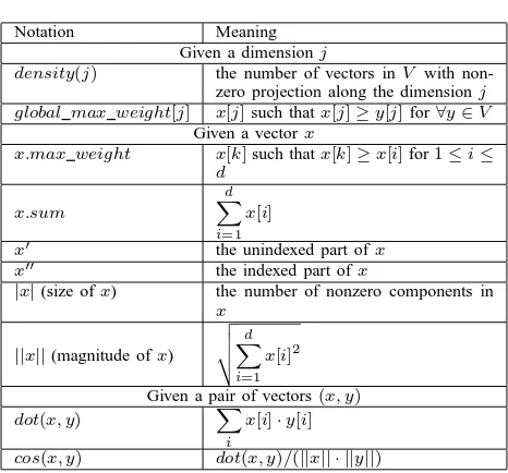
In this section, we define the problem and other important terms referred throughout the paper (please, see Table 1 for the summary of notations).
Definition 1 (All Pairs Similarity Search): The all pairs similarity search (AP SS) problem is to find all pairs(x, y)
and their exact value of similaritysim(x, y)such thatx, y ∈
V andsim(x, y) ≥t, where
• V is a set ofnreal valued, non-negative, sparse vectors
over a finite set of dimensionsD and|D|=d;
• sim(x, y) : V ×V →[0,1] is a symmetric similarity
function; and
• t,t∈[0,1], is the similarity threshold.
Definition 2 (Inverted Index): The inverted index maps each dimension to a list of vectors with non-zero projection along that dimension. A set of alldlistsI={I1, I2, ...., Id},
Table 1. Notations Used
Notation Meaning
Given a dimensionj
density(j) the number of vectors inV with non-zero projection along the dimensionj global max weight[j] x[j]such thatx[j]≥y[j]for∀y∈V
Given a vectorx
x.max weight x[k]such thatx[k]≥x[i]for1≤i≤ d
x.sum
d
X
i=1 x[i]
x′ the unindexed part ofx x′′ the indexed part ofx
|x|(size ofx) the number of nonzero components in
x
||x||(magnitude ofx)
v u u t
d
X
i=1 x[i]2
Given a pair of vectors(x, y)
dot(x, y) X
i
x[i]·y[i] cos(x, y) dot(x, y)/(||x|| · ||y||)
i.e., one for each dimension, represents the inverted index forV. Each entry in the list has a pair of values(x, w)such that if (x, w) ∈ Ik, then x[k] = w. The inverse of this
statement is not necessarily true, because some algorithms index only a part of each vector.
Definition 3 (Candidate Vector and Candidate Pair): Given a vector x∈ V, any vector y in the inverted index is a candidate vector for x, if ∃j such that x[j] > 0 and
(y, y[j])∈Ij. The corresponding pair (x, y)is a candidate
pair.
Definition 4 (Matching Vector and Matching Pair): Given a vectorx∈ V and the similarity thresholdt, a candidate vectory ∈V is a matching vector forx, if sim(x, y)≥t. We say that y matches with x, and vice versa. The corre-sponding pair (x, y)is a matching pair.
During subsequent discussions we assume that all vectors are of unit length (||x|| = ||y|| = 1), and the similarity function is the cosine similarity. In this case, the cosine similarity equals the dot product, namely:
sim(x, y) =cos(x, y) =dot(x, y).
We show the applicability of our algorithms for the Tanimoto coefficient similarity measure in Section 5.
3. Common Framework
Algorithm 1: Inverted index based framework common across recent exactAP SS algorithms
Input:V,t,D,sim,Ω,Π
Output:M AT CHIN G P AIRS SET
M AT CHIN G P AIRS SET = ∅;
1
Ii = ∅ ,∀ 1≤i≤d;
2
/* The inverted index is initialized
to d empty lists. */
Arrange vectors inV in the order defined by Ω;
3
Arrange components in each vector in the order
4
defined byΠ;
Computesummary statistics;
5
foreachx∈V using the order defined byΩdo 6
C = set of candidate pairs corresponding tox,
7
found by querying and manipulating the inverted indexI;
foreach candidate pair(x, y)∈C do 8
sim max possible= upper bound on
9
sim(x, y);
ifsim max possible≥t then 10
sim actual=sim(x, y);
11
ifsim actual≥t then 12
M AT CHIN G P AIRS SET = 13
M AT CHIN G P AIRS SET ∪ (x, y, sim actual)
14
15
foreachisuch thatx[i]>0using the order defined
16
byΠ do
iff iltering condition(x[i])is true then
17
Add(x, x[i])to the inverted index;
18
19
20
returnM AT CHIN G P AIRS SET
21
matching pairs. The framework can be broadly divided into three phases: data preprocessing, pairs matching, and indexing (please, refer to Algorithm 1 for details).
3.1. Preprocessing
The preprocessing phase reorders vectors using a permu-tationΩdefined overV (lines 1-5, Algorithm 1). Bayardo et al. [9] and Xiao et al. [10] sorted vectors on the maximum value within each vector. Sarawagi et al. [7] sorted vectors on their size. The components within each vector are also rearranged using a permutationΠdefined overD. Bayardo et al. [9] observed that sorting the dimensions inDbased on vector density speeds up theAP SS. The summary statistics about each record, such as its size, magnitude, and maximum component value are computed during the preprocessing phase. They are used later to derive filtering conditions
during the matching and indexing phases to save time and memory. The time spent on preprocessing is negligible compared to the time spent on matching.
3.2. Matching
The matching phase scans the lists in the inverted index that correspond to the non-zero dimensions in x, for a given vector x ∈ V, to find candidate pairs (lines 7-15, Algorithm 1). Simultaneously, it accumulates a partial similarity score for each candidate pair. Bayardo et al. [9] and Xiao et al. [10] used the hash-based map, while Sarawagi et al. [7] used the heap-based scheme for score accumulation.
Givent,Ω,Πandsummary statistics, various filtering conditions are derived to eliminate candidate pairs that will definitely not satisfy the required similarity threshold; these pairs are not added to the set C (line 7, Algorithm 1). Sarawagi et al. [7] identified the part of the given vector x∈ V such that for any candidate vector y ∈ V to have sim(x, y)≥t, the intersection of y with that part must be non-empty. Bayardo et al. [9] computed a lower bound on the size of any candidate vector to match with the current vector as well as any remaining vector. Our fast matching technique further tightens this lower bound.
Some of the candidate pairs can be safely discarded by computing an upper bound on the similarity score. Xiao et al. [10] used the Hamming distance based method for computing such an upper bound. But their technique and for-mulation of the APSS problem is specific to binary vectors only. Bayardo et al. [9] used the vector size and maximum component value to derive a constant time upper bound. We further tighten this upper bound in our fast matching technique. Finally, the exact similarity score is computed for the remaining candidate pairs, and those having scores above the specified threshold are added to the output set.
3.3. Indexing
The indexing phase adds a part of the given vector to the inverted index so that it can be matched with any of the remaining vectors (lines 16-20 Algorithm 1). Sarawagi et al. [7] unconditionally indexed every component of each vector. Instead of building the inverted index incrementally, they built the complete inverted index beforehand. Bayardo et al. [9] and Xiao et al. [10] used the upper bound on the possible similarity score with only the part of the current vector. Once this bound reached the similarity threshold, the remaining vector components were indexed.
4. Fast Matching
phase is critical for the running time. The computation time of the matching phase can be reduced in three ways:
• traversing the inverted index faster while searching for
candidate pairs,
• generating fewer candidate pairs for evaluation, and • reducing the number of candidate pairs that are
evalu-ated completely.
We propose two constant time optimizations that achieve these three goals, while guarantying not to eliminate any matching pair. Our tighter lower bound on the size of the candidate vector reduces the effective size of the inverted index, and the number of candidate pairs that are being generated. Our tighter upper bound on the similarity score reduces the number of candidate pairs that are being evalu-ated completely. First, we will prove the correctness of these bounds, and later we will show that they are tighter than the existing bounds.
4.1. Upper Bound on the Similarity Score
Given a candidate pair(x, y), the following constant time upper bound on the cosine similarity holds:
cos(x, y)≤x.max weight∗y.sum. (1)
The correctness of this upper bound can be derived from: x.max weight∗sum(y)≥dot(x, y) =cos(x, y). Similarly following upper bound can be derived:
cos(x, y)≤y.max weight∗x.sum. (2)
Combining upper bounds in 1 and 2, we propose following upper bound on cosine similarity score:
min(x.max weight∗y.sum, y.max weight∗x.sum), (3) whereminfunction selects minimum of the two arguments. We can safely prune the exact dot product computation of a candidate pair, if it does not satisfy the similarity threshold even for this upper bound.
4.2. Lower Bound on the Candidate Vector Size
For any candidate pair(x, y), the following is true: x.max weight∗y.sum≥dot(x, y).
For this candidate pair to qualify as a matching pair, the following inequality must hold:
y.sum≥t/x.max weight. For any unit-length vector y, the following is true:
y.sum≥k→ |y| ≥k2.
This gives us the following lower bound on the size of any candidate vectory:
|y| ≥(t/x.max weight)2. (4) The lower bound on the size of the candidate vector avoids generating the candidate pairs that will not satisfy the similarity threshold.
4.3. AP Time Efficient Algorithm
The proposedAP T ime Ef f icientalgorithm integrates both optimizations for the lower and upper bounds with the fastest-to-dateAll P airsalgorithm [9] (please, refer to Algorithm 2). The vectors are sorted in decreasing order of their max weight, and the dimensions are sorted in decreasing order of their vector density. For every x∈V, the algorithm first finds its matching pairs from the in-verted index (Matching Phase, Lines 6-22) and then adds selective parts ofx to the inverted index (Indexing Phase, Lines 23-29). The main difference between the algorithms AP T ime Ef f icient and All P airs is in the tighter bounds on filtering conditions. The correctness of these tighter bounds is proven above. Hence, the correctness of the AP T ime Ef f icientis the same as the correctness of theAll P airsalgorithm.
4.4. Tighter Bounds
The All P airs algorithm uses t/x.max weight as the lower bound on the size of any candidate vector. The AP T ime Ef f icient algorithm tightens this bound by squaring the same ratio (Line 8, Algorithm 2).
The All P airs algorithm uses the following constant time upper bound on the dot product of any candidate pair
(x, y):
min(|x|,|y|)∗x.max weight∗y.max weight. (5) We will consider following two possible cases to prove that our bound proposed in 3 is tighter than this bound.
• Case 1:|x| ≤ |y|
The upper bound in 5 reduces to:
|x| ∗x.max weight∗y.max weight. The upper bound proposed in 2 is tighter than this bound because:
x.sum≤ |x| ∗x.max weight.
• Case 2:|x|>|y|
The upper bound in 5 reduces to:
|y| ∗x.max weight∗y.max weight. The upper bound proposed in 1 is tighter than this bound because:
y.sum≤ |y| ∗y.max weight.
4.5. Effect on Matching Phase
For a given vector x, our proposed lower bound on the size of a candidate vector is inversely proportional to x.max weight. The vectors are sorted in decreasing order bymax weight. Hence, the value of the lower bound on the size of the candidate increases monotonically as the vectors are processed. If a vectorydoes not satisfy the lower bound on the size for the current vector, then it will not satisfy this bound for any of the remaining vectors. Such vectors can be discarded from the inverted index.
LikeAll P airs, our implementation uses arrays for rep-resenting lists in the inverted index. Deleting an element from the beginning of a list will have linear time overhead. Instead of actually deleting such entries, we just ignore these entries by removing them from the front of the list (Line 10, Algorithm 2). Because of our tighter lower bound on the size of the candidate, more such entries from the inverted index are ignored. This reduces the effective size of the inverted index, thus, resulting in faster traversal of the inverted index while finding candidate pairs. AP T ime Ef f icient also generates fewer candidate pairs as fewer vectors qualify to be candidate vectors because of the tighter lower bound on their size.
Computing the exact dot product for a candidate pair requires linear traversal of both vectors in the candidate pair (Line 20, Algorithm 2). The tighter constant time upper bound on the similarity score of a candidate pair prunes the exact dot product computation for a large number of candidate pairs. In our experiments we observed that AP T ime Ef f icientreduces the search space by at least an orders of magnitude (please, refer to Figure 4).
For the special case of binary vectors, where all non-zero values within a given vector are all equal, AP T ime Ef f icientwill not provide any speed up over All P airs because our optimizations depend on the vari-ation in the values of different components within a given vector.
5. Extension to the Tanimoto Coefficient
In this section, we extend AP T ime Ef f icient algo-rithm for the Tanimoto coefficient, which is similar to the extended Jaccard coefficient for binary vectors. Given a vector pair(x, y), the Tanimoto coefficient is defined as:
τ(x, y) =dot(x, y)/(||x||2+||y||2−dot(x, y)). First, we will show that τ(x, y)≤ cos(x, y). Without loss of generality, let||x||=a· ||y||anda≥1. By definition, it follows that:
cos(x, y)/τ(x, y) = (||x||2+||y||2−dot(x, y))/(||x||∗||y||),
= (a2+ 1)/a−cos(x, y),
≥(a2+ 1)/a−1,
Algorithm 2:AP T ime Ef f icientAlgorithm Input: V,t,d,global max weight,Ω,Π
Output:M AT CHIN G P AIRS SET
M AT CHIN G P AIRS SET = ∅;
1
Ii = ∅ ,∀1≤i≤d;
2
Ωsorts vectors in decreasing order by max weight;
3
Π sorts dimensions in decreasing order by density;
4
foreachx∈V in the order defined byΩdo 5
partScoreM ap = ∅;
6
/* Empty map from vector id to
partial similarity score */
remM axScore = 7
d
X
i=1
x[i]∗global max weight[i]; minSize = (t/x.max weight)2;
8
/* Lower bound on minimum size of
candidate is now squared */
foreachi: x[i]>0, in the reverse order defined by
9
Π do
Iteratively remove(y, y[i])from front ofIi
10
while|y|< minSize; foreach(y, y[i])∈Ii do
11
ifpartScoreM ap{y}>0 or
12
remM axScore≥t then
partScoreM ap{y} = 13
partScoreM ap{y} + x[i]∗y[i];
14
remM axScore = remM axScore − 15
global maximum weight[i]∗x[i];
/* Remaining maximum score that can be added after processing
current dimension */
foreachy:partScoreM ap{y}>0 do 16
ifpartScoreM ap{y} + min(sum(y′)∗
17
x.max weight, sum(x)∗y′.max weight)≥t
then
/* Tighter upper bound on the
similarity score */
s = partScoreM ap{y} + dot(x, y′);
18
ifs≥tthen 19
M AT CHIN G P AIRS SET = 20
M AT CHIN G P AIRS SET ∪ (x, y, s)
21
22
maxP roduct = 0;
23
foreachi: x[i]>0, in the order defined byΠdo 24
maxP roduct=maxP roduct+x[i]∗ 25
min(global max weight[i], x.max weight); ifmaxP roduct≥tthen
26
Ii = Ii∪ {x, x[i]};
27
x[i] = 0;
28
29
30
return M AT CHIN G P AIRS SET
≥1 + (a−1)2/a,
≥1.
Given the similarity thresholdt for the Tanimoto coeffi-cient, if we runAP T ime Ef f icient algorithm with the same threshold value for the cosine similarity, then they will not filter out any matching pairs. The only change we have to make is to replace the final similarity computation (Line 20 of Algorithms 2) with the actual Tanimoto coefficient computation as follows:
s=τ(x, y).
6. Experiments
1 10 100 1000 10000 100000 1e+06
1 10 100 1000 10000 100000
Frequency
Vector Size Medline
Flickr LiveJournal
Figure 2. Distribution of vector sizes
We empirically evaluate the effectiveness of our fast matching technique. We use the following abbreviations in figures for each algorithm:
• AP : All P airsalgorithm by Bayardo et al. [9]; and • APT : AP T ime Ef f icientalgorithm.
We performed experiments on three real-world data sets for both the cosine similarity and the Tanimoto coefficient. Results for both similarity measures are quite similar. In this paper, we present results only for cosine similarity for the sake of brevity. More details about results for the Tanimoto coefficient can be downloaded from the Web [15]. Many practical applications need pairs with relatively high similarity values [3], [2], [10], [1]. Hence, we varied the similarity threshold from 0.8 to 0.99 in 0.05 increments.
All our implementations are in C++. We used the standard template library for most of the data structures. We used the dense hash mapclass from GoogleT M for the hash-based partial score accumulation [16]. The code was compiled using the GNU gcc 4.2.4 compiler with −O3 option for optimization. All the experiments were performed on the same 3 GHz Pentium-4 machine with 4 GB of main memory. The code and the data sets are available for download on the Web [15].
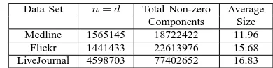
Table 2. Data Sets Used
Data Set n=d Total Non-zero Average Components Size Medline 1565145 18722422 11.96
Flickr 1441433 22613976 15.68 LiveJournal 4598703 77402652 16.83
6.1. Data Sets
Out of the three data sets, one comes from the scien-tific literature collaboration information in Medline indexed papers [11]. The rest come from the popular online social networks, Flickr [12] and LiveJournal [13]. These data sets were chosen, because they represent variety of large-scale web-based applications like digital libraries and online social networks, that we are primarily interested in. The observed distribution of the vector sizes in the data sets is the power law distribution [17] (please, refer to Figure 2). These data sets are high dimensional and sparse (please, refer to Table 2). The ratio of the average size of vector to the total number of dimensions, is less than 10−4. All these characteristics are common across data sets generated and used by many large-scale web based applications [9], [18]. These applications have to solve the APSS problem for high-dimensioanl data sets with millions of records; which are often sparse. Therefore, our fast matching technique will be relevant for other similar data sets as well.
6.1.1. Medline. This data set was selected to investigate possible applications for large web-based scientific digital libraries like PubMed, ACM Digital Library, and CiteSeer. Such digital libraries help users to find similar publications and authors. We used the data set prepared by the Auton Lab of Carnegie Mellon University. We are interested in finding pairs of authors that have similar collaboration patterns. Each vector represents the collaboration pattern of an author over the space of all authors. Two authors are considered to be collaborators if they write at least two papers together. Similar strategies were used in previous work [9] to eliminate accidental collaborations. We use the weighing scheme of Newman [19] to derive the weight of collaboration between any two authors. Ifkauthors have co-authored a paper, then it adds1/(k−1)to the collaboration weight of each possible pair of authors of that paper. All vectors are then normalized to unit-length.
100000 1e+06
0.8 0.9 0.95 0.99
Medline
AP APT
1e+06 1e+07
0.8 0.9 0.95 0.99
Flickr
AP APT
100000 1e+06 1e+07
0.8 0.9 0.95 0.99
LiveJournal
AP APT
Figure 3. Ignored Entries from Inverted Index vs. Similarity Threshold for Cosine Similarity
100000 1e+06 1e+07 1e+08
0.8 0.9 0.95 0.99
Medline
AP APT Actual Matching Pairs
1e+06 1e+07 1e+08 1e+09
0.8 0.9 0.95 0.99
Flickr
AP APT Actual Matching Pairs
100000 1e+06 1e+07 1e+08 1e+09
0.8 0.9 0.95 0.99
LiveJournal
AP APT Actual Matching Pairs
Figure 4. Candidate Pairs Evaluated vs Similarity Threshold for Cosine Similarity
100 120 140 160 180 200 220 240 260
0.8 0.9 0.95 0.99
Medline
AP APT
100 200 300 400 500 600 700 800
0.8 0.9 0.95 0.99
Flickr
AP APT
200 250 300 350 400 450 500 550 600 650
0.8 0.9 0.95 0.99
LiveJournal
AP APT
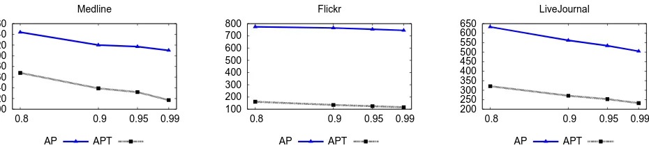
Figure 5. Runtime in Seconds vs. Similarity Threshold for Cosine Similarity
vector has non-zero projection along those dimensions that correspond to the users in his/her friend list. But the weights of these social network links are unknown. So, we applied the weight distribution from the Medline data set to assign the weights to these social network links in the two data sets. To ensure that our results are not specific only to the selected weight distribution, we also conducted experiments by generating the weights randomly. The results were similar and are available on the Web [15].
6.2. Fast Matching Performance
We evaluate the performance of fast matching in theAP T ime Ef f icientalgorithm based on three parameters: the size of the inverted index, the size of the search space, and the end-to-end run-time. The preprocessing phase is identical
in both algorithms. The time spent on data preprocessing was negligible as compared to the experiments’ running time, and was ignored. Though the indexing phase is also identical in both algorithms, the time spent in indexing phase was considered in the end-to-end running time, as it was not negligible.
end-to-end speed up, because some time is still spent traversing the inverted index to find candidate pairs and filtering out a large fraction of them.
The best speed up is obtained for the Flickr data set, because it has a heavy tail in the distribution of vector sizes (please, refer to Figure 2). Vectors having the long size typically generate a large number of candidate pairs. But AP T ime Ef f icient effectively avoids their generation and evaluation. In fact, for the Flickr data set, the number of candidate pairs evaluated byAP T ime Ef f icientalmost equals the actual number of matching pairs (please refer to Figure 4).
7. Conclusion and Future Work
We described the inverted index based framework com-mon across recent exact algorithms for all pairs similarity search. Within this framework, we presented tighter bounds on the candidate size and similarity score. These bounds reduced the search space by at least an order of magnitude and provided significant speed up for three large real-world data sets. Our fast matching technique will be relevant for other similar data sets, which are frequent across many web based systems.
Incremental formulations of APSS where APSS is per-formed multiple times over same data set while varying the similarity threshold, is an interesting problem for future work. Incremental algorithms would potentially save a lot of repetitive computation across multiple invocations of APSS. Parallelizing the solutions for APSS is an important unexplored direction. It would enable us to take advantage of high performance computing infrastructure to process larger data sets, which otherwise cannot be processed in reasonable time sequentially.
8. Acknowledgments
We thank Paul Bremiyer of NCSU for thoughtful com-ments and suggestions. We are also thankful to the Auton Lab of Carnegie Mellon University and Max Planck Institute for Software Systems for making their data sets publicly available. This work is performed as part of the Scientific Data Management Center (http://sdmcenter.lbl.gov) under the Department of Energys Scientific Discovery through Advanced Computing program (http://www.scidac.org). Oak Ridge National Laboratory is managed by UT-Battelle for the LLC U.S. D.O.E. under contract no. DEAC05-00OR22725.
References
[1] S. Chien and N. Immorlica, “Semantic similarity between search engine queries using temporal correlation,” in WWW
’05.
[2] E. Spertus, M. Sahami, and O. Buyukkokten, “Evaluating similarity measures: a large-scale study in the orkut social network,” in ACM SIGKDD ’05.
[3] H. Li, I. G. Councill, L. Bolelli, D. Zhou, Y. Song, W.-C. Lee, A. Sivasubramaniam, and C. L. Giles, “Citeseerχ: a scalable
autonomous scientific digital library,” in InfoScale ’06.
[4] M. S. Charikar, “Similarity estimation techniques from round-ing algorithms,” in STOC ’02.
[5] A. Z. Broder, S. C. Glassman, M. S. Manasse, and G. Zweig, “Syntactic clustering of the web,” Comput. Netw. ISDN Syst., vol. 29, no. 8-13, pp. 1157–1166, 1997.
[6] R. Fagin, R. Kumar, and D. Sivakumar, “Efficient similarity search and classification via rank aggregation,” in ACM
SIGMOD ’03.
[7] S. Sarawagi and A. Kirpal, “Efficient set joins on similarity predicates,” in ACM SIGMOD ’04.
[8] A. Arasu, V. Ganti, and R. Kaushik, “Efficient exact set-similarity joins,” in VLDB ’06.
[9] R. J. Bayardo, Y. Ma, and R. Srikant, “Scaling up all pairs similarity search,” in WWW ’07.
[10] C. Xiao, W. Wang, X. Lin, and J. X. Yu, “Efficient similarity joins for near duplicate detection,” in WWW ’08.
[11] “Medline literature database of life sciences and biomedi-cal information : www.nlm.nih.gov/pubs/factsheets/medline. html.”
[12] “Flickr online photo sharing social network : www.flickr. com/.”
[13] “Livejournal blogging social network : www.livejournal. com/.”
[14] H. Turtle and J. Flood, “Query evaluation: strategies and optimizations,” Inf. Process. Manage., vol. 31, no. 6, pp. 831– 850, 1995.
[15] “Code and data sets for our algorithms : www4.ncsu.edu/
∼acawekar/.”
[16] “Google dense hash map library : code.google.com/p/ google-sparsehash/.”
[17] A. Mislove, M. Marcon, K. P. Gummadi, P. Druschel, and B. Bhattacharjee, “Measurement and analysis of online social networks,” in ACM IMC ’07.
[18] A. Broder, R. Kumar, F. Maghoul, P. Raghavan, S. Ra-jagopalan, R. Stata, A. Tomkins, and J. Wiener, “Graph structure in the web,” in WWW ’2000.
[19] M. E. J. Newman, “Scientific collaboration networks. ii. shortest paths, weighted networks, and centrality,” Physical