The Development of Textile Based Acoustic Sensing Arrays for Sound Source Acquisition

(1)

Abstract

Luthy, Kyle Anthony. The Development of Textile Based Acoustic Sensing Arrays for Sound Source Acquisition. (Under the direction of Dr. Edward Grant.)

This research project dealt primarily with the production of an electronic textiles

(e-textiles) demonstrator. The goal of electronic textiles is to integrate textiles technology and

electronics to create large area conformal surfaces with embedded electronics. Here, the

e-textiles demonstrator serves as an acoustic array for sound source localization and tracking.

To create portable acoustic arrays on a flexible textile substrate, an understanding of textile

designs and textile processes was obtained. This research resulted in the fabrication of

woven substrates with conducting lines and embedded microphone windscreens. Similarly,

an understanding of the design and manufacture of flexible substrates for electronics had to

be gained in order to produce miniature electronic circuits that will flex when embedded in a

textile substrate. The acoustic array technology developed includes microphone arrays with

their associated software for data capture and analysis, a multiplexer circuit on a flexible

Kapton substrate, and a UC-Berkeley mote-based technology for use with a custom miniature

microphone amplification system.

Ultimately, these arrays are used to demonstrate sound localization by triangulation as

well as via the spatial filtering technique of beamforming. Experiments were performed to

compare different array sizes and geometries in both simulation and real world practice for a

variety of target frequencies. Mote performance in the role of beamforming is compared to

simulation as well as a commercially available system. Although not as ideal as in

simulation, the results achieved are comparable to those of the professional system tested

(2)

The Development of Textile Based Acoustic Sensing Arrays for Sound

Source Acquisition

by

Kyle Anthony Luthy

A thesis submitted to the Graduate Faculty of North Carolina State University

in partial fulfillment of the requirements for the Degree of

Master of Science

COMPUTER ENGINEERING

Raleigh

2003

(3)

Biography

Kyle Anthony Luthy was born January 6, 1978 in Omaha, Nebraska. Shortly

thereafter his family moved to Baton Rouge, Louisiana where he eventually would attend

Louisiana State University (LSU). While enrolled at LSU, Kyle was an active member of

Theta Xi Fraternity, IEEE, Habitat for Humanity, Eta Kappa Nu, and Golden Key. In May of

2001 he was inferred Bachelor’s degrees in Electrical Engineering, Computer Engineering,

and Computer Science. His interest in robotics then led him to North Carolina State

University to pursue a Master’s degree in Computer Engineering. At NCSU he is affiliated

with the Center for Robotics and Intelligent Machines under the direction of Dr. Edward

Grant. His work has focused on mobile robotic systems, acoustic sensing, electronic textiles,

(4)

Acknowledgements

It is appropriate that I first recognize Dr. Edward Grant, my advisor and director of

the Center for Robotics and Intelligent Machines. I thank him for his support and confidence

in my abilities. I would like to also thank my committee members, Dr. John Muth, Dr.

Benham Pourdeyhimi, and Dr. Troy Nagle, for their ideas concerning this thesis as well as

providing direction for future research.

I would have accomplished little without the assistance of all of the members of the

CRIM. It’s a rare opportunity to be able to work with such a talented group. It is safe to say

that I have learned more from working with this group of individuals than I could have in any

classroom. I would particularly like to recognize the contributions of Chris Braly and

Leonardo Mattos from the CRIM and Anuj Dhawan from the College of Textiles for their

assistance.

It is also important to note the contributions of my family, while not directly involved

with the content of this thesis, they are ultimately responsible for its foundation. I would like

to thank my mother for her patience, encouragement, and good cooking; my father for his

unwillingness to let me accept things without asking why, and my sister for the shining

(5)

List of Figures

Figure 2.1 A Flexible PDA keyboard utilizing SOFTSwitch technology [10]... 7

Figure 2.2 Infineon's MP3 Jacket can be washed and ironed. ... 8

Figure 2.3 Georgia Tech's Smart Shirt is used to monitor the wearer's vital signs. ... 9

Figure 2.4 GUARDIAN sniper detection system. ... 10

Figure 2.5 Acoustic array necklace for the hearing impaired... 11

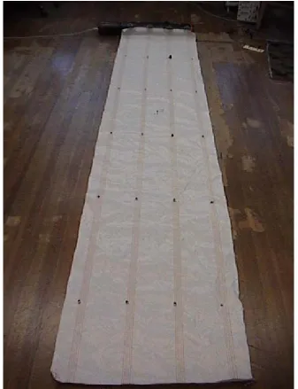
Figure 3.1 The 1st generation 10ft, 20 element, textile based acoustic array... 12

Figure 3.2 Camouflage array with woven windscreens. 1 is an unprotected mic, 2 has a lavalier windscreen, 3 is a loosely woven windscreen, and 4 is a tight woven windscreen. ... 14

Figure 3.3 Oscilloscope screen shot demonstrating the performance of the windscreen usage of figure 3.1. Channel 1 has no windscreen, channel 2 has a lavalier windscreen, 3 is loosely woven, and 4 is tightly woven. (Gain of 100) ... 14

Figure 3.4 Textile array containing both microphones and amplifiers on fabric... 16

Figure 3.5 Floats woven for device attachment. ... 17

Figure 3.6 Coaxial snap connector for microphone attachment. ... 17

Figure 3.7 Emkay microphone WP-3502. ... 18

Figure 3.8 Panasonic microphone WM52B... 18

Figure 3.9 Frequency response of the Panasonic WM52B microphone... 18

Figure 3.10 Microphone and non-inverting amplifier with gain of 100. ... 18

Figure 3.11 Hoontech/Staudio audio mixer ...Error! Bookmark not defined. Figure 3.12 Configuration of the 4 element array... 23

Figure 3.13 Simulated beamforming on 1KHz source at 90 degrees azimuth and no elevation. The result matches the actual location. ... 24

Figure 3.14 Real world beamforming on 1KHz source at 90 degrees azimuth and no elevation. The sound source is detected at an azimuth of 90 degrees and an elevation of 10 degrees. ... 24

Figure 3.15 Frequency spectrum of one of the signals contributing to the beam pattern of figure 3.14... 25

Figure 3.16 Real world result after introducing a software filter. Sound source is at 90 degrees azimuth and no elevation. The sound source is detected correctly... 26

Figure 3.17 Simulation with sound source located at 90 degrees azimuth and 25 degrees elevation. Detected at an azimuth of 200 degrees and elevation of 50 degrees... 27

Figure 3.18 Listening pattern using a three dimensional array. Source location and detected location are identical at 90 degrees azimuth and 25 degrees elevation. ... 27

Figure 3.19 Triangulation electronics housed in a blueprint tube. ... 29

Figure 3.20 Block diagram of circuitry used to measure time delays for triangulation ... 29

Figure 4.1 The mote based acoustic sensing system... 31

Figure 4.2 The Rene mote developed by Jason Hill at UC Berkeley. Top (left), bottom (right) ... 33

Figure 4.3 Flexible data acquisition circuit on a Kapton substrate... 34

(8)

Figure 4.5 Multiplexer noise reduces with lower frequency but is still prevalent. Yellow -

clock, Blue - output... 37

Figure 4.6 Kapton based circuit sewn into a miniature array. ... 38

Figure 4.7 Flexibility demonstration of the Kapton based circuit. ... 38

Figure 4.8 The 8 channel variable gain data acquisition circuit. ... 39

Figure 4.9 Protoboard data acquisition circuit... 41

Figure 4.10 4x5 array configuration of the 1st generation array shown in figure 3.1. ... 42

Figure 4.11 Beam Forming Simulations for the Rectangular Array of figure 4.10. Multiple beams are observed with a 1kHz sound source at 90 degrees (left) but are not present when located at 0 degrees (right)... 43

Figure 4.12 8 element array configuration for mote based sensing... 44

Figure 4.13 Beam Forming Simulations of 8 Element Circular Array at 0, 45, and 90 degrees Respectively given a 1kHz sound source... 44

Figure 4.14 Oscilloscope screen shot displaying the sampling frequency used to sample the acoustic source (top) and the sampling time used to sample the 8 microphone elements (bottom)... 47

Figure 4.15 Program Flow Chart for a Sensor Array... 48

Figure 4.16 Simulated sound recordings (left) and real world sound recordings (right)... 54

Figure 4.17: Frequency spectra of (a) tank, (b) truck, (c) helicopter, (d) missile, and (e) gun shot [46] ... 60

Figure 4.18 Samples of a 100Hz sound source taken at 44100Hz using the Hoontech data acquisition system... 63

Figure 5.1 Demonstration of a Leno weave. [1] ... 68

Figure 5.2 Triangulation of sound source position using two acoustic arrays of known position... 70

Figure 5.3 Demonstration of beam thinning using information from multiple arrays to form the same beam-pattern. ... 71

Figure A.1-1 Schematic for the Rene mote designed by Jason Hill of UC Berkeley... 78

Figure A.1-2 Composite of all PCB layers for the Rene mote ... 79

Figure A.1-3 Top PCB layer of the Rene mote. ... 79

Figure A.1-4 First inner PCB layer of the Rene mote. ... 79

Figure A.1-5 Ground plane PCB layer of the Rene mote. ... 80

Figure A.1-6 Second inner PCB layer of the Rene mote... 80

Figure A.1-7 Bottom PCB layer of the Rene mote... 80

Figure A.2-1 Composite PCB layout for the Rene programming board ...86

Figure A.2-2 Top layer PCB layout for the Rene programming board ...86

Figure A.2-3 Bottom layer PCB layout for the Rene programming board...86

Figure A.3-1 Composite PCB layout of the serial communications board...89

Figure A.3-2 Top PCB layer of the serial communications board ...89

Figure A.3-3 Bottom PCB layer of the serial communications board...89

Figure A.4-1 Schematic for the flexible data acquisition circuit ...91

Figure A.4-2 PCB layout for the flexible data acquisition circuit ...92

Figure A.5-1 Circuit schematic for the variable gain data acquisition system ...97

Figure A.5-2 Composite PCB layout of the variable gain data acquisition system...98

Figure A.5-3 Top PCB layer copper and silk from figure A.5-2...98

(9)

List of Tables

Table 4.1 Beam-patterns with varying sampling times taken of a 1kHz source at a rate of

12.5kHz... 51

Table 4.2 Beam-patterns with varying sampling times taken of a 100Hz source at a rate of 12.5kHz... 52

Table 4.3 Effects of a sampling period of 0.0124s for various sampling and source frequencies. ... 53

Table 4.4 Simulated and actual beam-patterns realized from various target frequencies at both 0 and 185 degrees. ... 55

Table 4.5 Inconsistent results after sampling a 1KHz source located at 0 degrees. ... 58

Table 4.6 Beam patterns for various sound sources located at 0 degrees... 59

Table 4.7 Demonstration of inconsistent beam patterns formed on truck sounds located at 0 degrees. ... 62

Table 4.8 Beam patterns achieved by sampling at 44100Hz for 1s with the Hoontech system. ... 64

Table A.1-1 Materials listing for the Rene mote. ... 81

Table A.2-1 Materials listing for the Rene programming board. ... 88

Table A.3-1 Materials listing for the mote serial communications board. ... 91

Table A.4-1 Materials listing for the flexible data acquisition circuit... 93

(10)

Chapter 1 – Introduction

Distributed sensor systems can provide a tremendous amount of information regarding

one’s environment. Whether embedded in a building or strewn across miles of countryside,

they can tell us the temperature gradient, determine the chemical composition of the air,

detect seismic activity, or simply listen to the surrounding environment to provide sound

localization. The more sensors of a similar type deployed in a given area, the higher quality

the data collected is in terms of resolution and redundancy. To further improve on data

quality, it is often desirable to have sensing systems arranged in arrays where geometry can

be utilized to maximize performance. An example would be an even sensor distribution over

a field to map moisture content. If the distribution is uneven (irregular) then more

information will be gathered about one particular area than another.

This thesis is dedicated in particular to acoustic sensor arrays. Such arrays are useful for

spatial filtering of sound data, also referred to as beamforming. In other words, they

facilitate directional listening without the use of parabolic microphones. Array geometry has

an effect on the detectable frequency of the system such that sensor elements should be

spaced apart by λ/2 where λ is the wavelength of the lowest frequency sought. This thesis

addresses the use of an individual array; one single element in what in the future will be a

distributed system. This is useful since although each array in a distributed system will

provide a relative direction to a sound source, they cannot effectively provide distance

(11)

characterized). Using directional information gathered from multiple arrays the distance to

the sound source can be triangulated.

The use of textiles as a substrate for sensor arrays is also examined to provide them with

flexibility and portability. The ability to fold a large area array is particularly useful to a

soldier deploying distributed sensor systems in the field, as it is less cumbersome than would

be a rigid substrate. This allows for the deployment of larger arrays to improve performance.

Textiles are also relatively light which is important as a soldier can already be carrying

upwards of 100lbs of personal equipment [1]. Since the sensor elements are already laid out,

the soldier does not have to measure and place each individual element upon deployment, as

is the current mode of deploying an acoustic array. The focus here is on rapid deployment

and portability. Embedding such systems in textiles also allows for their non-intrusive

inclusion in tents, parachutes, and truck coverings. This can likewise be applied in buildings,

through embedding sensor arrays in rugs or drapes in a dwelling or workplace. Sensor arrays

can be rolled out during construction and embedded into walls to enhance conference room

acoustics, in bridges to measure stress levels, as well as any number of homeland security

applications.

1.1 Military Motivation for the Use of Distributed Sensing

Historically, the military powers of the world have adopted the use of defense barriers to

deter invading armies. By far the most effective of such barriers was the Morice Line

constructed in 1957 by the French to protect their colonial interests in Algeria from Algerian

nationalists. This fortification spanned 460km along the Tunisian border and 750km along

(12)

eight foot, 5000 volt electric fence. The line was manned by 80,000 French troops and

patrolled aerially. Algerian nationalist infiltration was effectively countered [2].

Encouraged by such successes, the United States attempted a similar barrier in Vietnam.

The McNamara Line was to expand along the demilitarized zone between North and South

Vietnam as well as the Laotian border. Along with the traditional barbed wire and mines,

acoustic and chemical sensors were also to be deployed. Although the McNamara Line is

considered a failure and was never completed, the sensor technologies implemented proved

to be beneficial. Seismic and acoustic sensors were utilized in the defense of Khe Sanh

where “the sensors indicated when the enemy were massing for attacks against the base,

allowing the concentrated deployment of US aerial and artillery bombardment which

countered the attack…defenders at Khe Sanh did not face their enemy across a broad, linear

front; rather, they were almost surrounded by them. The fighting there showed that sensor

technology worked in 360-degree applications [2]”. Such sensors were further activated for

operations along the Ho Chi Minh trail after which only an estimated 20 percent of vehicles

reached their objective [2] [3].

Within the last 20 years there has been a push towards improving US implementation of

the electronic barrier concept. The rapid deployability of the US military once a target has

been electronically acquired drastically reduces the need for manpower along the protected

border. Also, determining patterns of troop and equipment movement allows for better

localization of mines and physical barriers [3]. Not only is this cheaper, but it also reduces

the post war impact of munitions left on the battlefield. According to the 2000 Land Mine

Monitor Report, there are approximately 1.3 million mines still in place in Algeria. Along

(13)

meter [4]. While a wall may impede insurgent forces, once in place and mines are laid,

counter-invasion plans will also be restricted.

Furthermore, in the past few years there has been a substantial push within the US armed

forces towards what is termed the Objective Force Warrior. The premise behind this project

is to use technology to increase the effectiveness of individual soldiers. This is largely

accomplished by inundating soldiers with information gained from various sensors,

providing them with a more comprehensive view of the battlefield [5]. Sensor arrays can

provide target information as well as detect the use and density of biological agents.

1.2 Goals of Thesis

The objectives of this thesis are

• Describe the development of a large area textile based triangulation array.

• Develop a beamforming array sensor system based on UC Berkeley’s mote.

• Examine flexible circuitry implemented on a Kapton substrate.

• Develop a miniature variable gain data acquisition system for the mote.

• Demonstrate beamforming for sound source localization.

1.3 Thesis

Outline

• Chapter 2 - A literature review highlighting current research and applications of

electronic textile technologies and acoustic arrays.

• Chapter 3 - A detailed examination of the design and implementation of a 10’ x 3’

microphone array for sound impulse location through triangulation based on time

(14)

computer based beamforming system. This includes different wiring techniques,

the characterization of woven windscreens, and the development of the associated

electronics.

• Chapter 4 – The development of a mote based beamforming array. This includes

information regarding the Berkeley mote, the determination of the array

geometry, the design and implementation of a flexible data acquisition circuit, the

design and implementation of a variable gain data acquisition circuit, software

development, and experimentation evaluating performance.

• Chapter 5 - Conclusions and future work.

• Appendix A - Circuit schematics, board layouts, and material listings for

developed circuitry.

(15)

Chapter 2 – Literature Review

This chapter investigates many of the recent technological advances and current

research interests in the fields of electronic textiles and acoustic arrays. This review provides

a wide view of these areas and is not restricted to information pertinent to the content of this

thesis.

2.1 Electronic Textiles

Electronic textiles are created in an effort to incorporate computer technology into a

medium with which we are already familiar and to do so in a non-intrusive manner. “Textile

look and feel must not be impaired by new functions, which means that technology must be

small, light-weight and smooth. Mechanical stress must not lead to failure, washing and

cleaning must be possible.” – Siglinde Zisler [6]. Such requirements have created many

challenges for researchers who have answered with imaginative innovations, bringing these

goals closer to fruition.

To obtain seamless integration, technologies are required from various disciplines,

including textiles, materials, and electronics. Textile engineers and materials scientists have

developed several methods for integrating conductors into textile substrates. Optical fibers,

metallic or composite fibers, and yarns coated with conductive polymers can be woven or

embroidered into the fabric to create transmission lines or circuit layouts [7] [8] [9].

Conductors can also be included in the manufacture of non-woven textiles such as in

(16)

making electric blankets. Conductive inks and dyes can also be used to introduce conductors

to a textile [7].

To be better suited for inclusion in textiles, electronic components need to be either

smaller than or as flexible as the fabric in which they are embedded. Current minimization

trends in electronics have produced much in the areas of both micro and nanometer (nano)

scale devices which are well suited for seamless inclusion in textile substrates. Others utilize

special fibers sewn in a particular configuration to create the desired device. Such a

component is demonstrated by the SOFTSwitch (figure 2.1). The SOFTSwitch uses

conductive materials and a quantum tunneling composite to allow resistance to change with

pressure [10] [11]. Fitting with the theme of sensing arrays, this technology can be applied to

pressure mapping; a useful feature for medical applications.

Figure 2.1 A Flexible PDA keyboard utilizing SOFTSwitch technology [10].

Power consumption must also be minimal to avoid the need for large battery packs.

To help solve this problem, Infineon has developed a thermogenerator which utilizes body

heat to generate electricity. Currently, enough energy is produced to power either a digital

(17)

based on light harvesting dyes [13]. Flexible battery technology is currently available from

Power Paper Ltd. whose thin batteries are printed onto the desired substrate [14].

The current focus of electronic textile application both commercially and in research

is on wearable devices. There are many commercially available items in which electronic

devices have been embedded [12] such as Infineon’s mp3 player jacket (figure 2.2) [11],

Northface’s MET5 heated jacket [15], and the Polartec electric blanket [16]. The

development of such products fuels the current trend of smaller, more robust electronic

components.

Figure 2.2 Infineon's MP3 Jacket can be washed and ironed.

Research “wearables” typically focus on health and military applications rather than

fashion and entertainment. The Georgia Institute of Technology (Georgia Tech) Smart Shirt

for example, is a T-shirt into which various sensors are woven to monitor several vital signs

(figure 2.3) [17]. Likewise, researchers at Wollongong University in Australia utilize yarns

coated with inherently conducting polymers (ICP) which they imbed into their Knee Sleeve

(18)

[18]. Other research focuses on embedded actuators [19] [20], electrically controlled

camouflage [21], and wearable displays [22].

Figure 2.3 Georgia Tech's Smart Shirt is used to monitor the wearer's vital signs.

Many of the aforementioned technologies are funded by the Natick Soldier Center as

a part of their Objective Force Warrior initiative [5]. This program strives to provide the

soldier with all pertinent information about their environment as well as defend them from

harm by including advances such as adaptive camouflage, automatic tourniquets, and vital

sign monitoring directly into their uniform. DARPA has also funded electronic textile

projects not involving wearable systems. This includes research on controllable parafoils and

large area acoustic arrays for vehicle detection which has been performed concurrently at

North Carolina State University [13] [23] and Virginia Tech [24]. This work is discussed in

(19)

2.2 Acoustic Arrays

Since the 60’s, the United States military has been looking to mimic the successes of

passive sonar technologies on land in order to improve the localization and tracking of

military units. Throughout the 1980’s and early 1990’s, sensor systems such as REMBASS

(Remote Battlefield Sensor System) [25] and later IREMBASS (Improved REMBASS) were

developed. More recently, the United State’s Army Research Lab and several NATO nations

have focused on Unattended Ground Sensors (UGS) which are smaller than the REMBASS

systems and are more easily deployed [26]. These systems typically comprise a variety of

sensors in addition to acoustic sensors including seismic, chemical, and biological. The

Army Research Lab (ARL) is actively examining acoustic arrays for addition into such

systems since although current systems are useful for providing a large amount of

information, they cannot reproduce the spatial discrimination of an acoustic array.

Consequently, the ARL is responsible for a large amount of literature on acoustic array

processing techniques [27][28][29]. DRDC Valcartier, a Canadian defense contractor, is

responsible for the development of free standing and vehicle mounted acoustic arrays [30].

One such system is GUARDIAN (figure 2.4) which is used for sniper localization.

(20)

Mounting arrays on vehicles can be particularly challenging, not only because the

system is moving, but vehicles are often inherently noisy [31]. This is likewise a challenge

when including such arrays on robotic platforms. Arrays are incorporated into robots which

are used for surveillance, search and rescue, and target localization and tracking [32][33][34].

With advances in computing power and electronic minimization, acoustic arrays have

been applied to various tasks involving speech processing [35]. This is rather difficult as

human speech encompasses a rather large range of frequencies. Work with array geometries

[35] and processing techniques [36][37][38] has aided in the development of products that

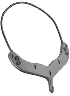
approve acoustics in conference rooms [39][40] or aid the hearing impaired such as the

microphone array necklace shown in figure 2.5 [41].

(21)

Chapter 3 – 1

st

Generation System Designs

This chapter examines the development of the first generation acoustic array

constructed on a textile substrate. This system was designed and implemented as part of a

DARPA funded project and has been the subject of several papers [23][8]. The final design

is shown in figure 3.1.

(22)

3.1 Textile

Considerations

The textile requirements for this project vary considerably from those associated with

typical fashion directed electronic textiles. Durability is more important than style since

there are no comfort issues involved with the associated wiring and embedded electronics.

3.1.1 Designing a Substrate for E-Textile Usage

The textile substrate for the array was chosen to be polyester. Polyester is a popular

fabric for military applications as it is lightweight (approximately 16g/m2), strong, has good

abrasion resistance, displays uniform characteristics, and is resistant to moisture and other

environmental conditions [42]. It is also a fairly simple material to dye in order to provide

camouflage in the visible spectrum. Larger area arrays would also need to consider

reflectance in the near infrared wavelengths (.7-2um) due to the high infrared reflectance

typical of vegetation. Pigment printing techniques for polyester utilizing azoic colorants or

isoindolinone residues to reduce NIR reflectance have been developed [42].

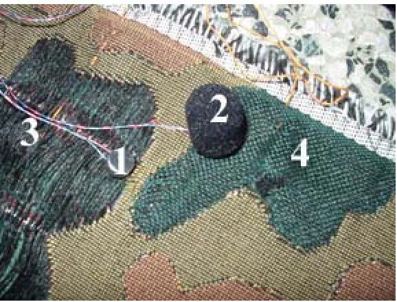
A camouflage array was woven on a Jacquard loom and is shown in figure 3.2. This

array also has pockets woven into it of various densities. These pockets not only conceal the

microphone elements, they also serve as windscreens. This does however have an adverse

effect on electronic interfacing in that the wires are not easily accessible. To test the

effectiveness of the woven windscreens, their performance is compared to that of a

microphone with no windscreen and one with a WindTech™ lavalier windscreen. Using a

compressed air source the microphones were simply grouped closely together and they were

blown upon. The wind speed was regulated by measuring with an anemometer and sustained

approximately at 275 ft/min. The results are shown below in the oscilloscope screen shot of

(23)

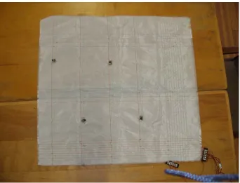
Figure 3.2 Camouflage array with woven windscreens. 1 is an unprotected mic, 2 has a lavalier windscreen, 3 is a loosely woven windscreen, and 4 is a tight woven windscreen.

(24)

As can be seen, the microphone with the lavalier windscreen outperforms the others. As

expected, the unprotected microphone yielded the worst performance. The tightly woven

windscreen performed slightly better than did the loosely woven. This test was performed

several times with comparable results. The sound acceptance of the microphones was also

tested since a windscreen is not effective if it degrades the signal it is intending to pick up.

At various frequencies between 20Hz and 500Hz, no appreciable differences in microphone

performance were detected.

3.1.2 Wiring

The wiring necessary for the array depends on the complexity of the circuitry which

is to reside on the fabric. The preliminary design had each microphone and its associated

amplifier collocated on the fabric. This type of node requires individual power, ground, and

signal lines. The resulting wiring grid is shown in the 4-element prototype pictured in figure

3.4. The spacing of the wires was chosen to be commensurate with the findings of [9] to

reduce crosstalk. All of the wires utilized were stranded to improve flexibility and consisted

of bare copper, insulated copper, and twisted pair wires. These wires are all of 36 gauge or

smaller in order to pass through the reed of the loom that was available. The twisted pair is

particularly important as it carries the resulting signal to some processing station. While not

critical in this small design, when scaled upwards, the twisted pair serves to protect signal

integrity over large distances. Further, it is important to note the need of interconnections

between wires in this design. Interconnects in this array were solder welded but several other

(25)

Figure 3.4 Textile array containing both microphones and amplifiers on fabric.

The second and final design removed the amplification from the on fabric node. With

this reduced circuit complexity, the necessity for interconnects and wires woven in the weft

are removed. Only the twisted pair wires remain as is demonstrated in the finished product

of figure 3.1.

3.1.3 Interfacing

Forming external connections to the woven wires requires special consideration.

Weaving can be done to facilitate the attachment of node elements by allowing the wire to

float at the attachment points (figure 3.5). Also a co-axial snap connector was developed for

external device connection (figure 3.6). Not only does such a connection allow for the easy

replacement of an element, it also reduces stresses on the wire and distributes them to the

(26)

Figure 3.5 Floats woven for device attachment. Figure 3.6 Coaxial snap connector for microphone attachment.

3.2 Microphones and Amplifiers

To perform well the microphones incorporated into the array must be both small and

have an acceptable signal to noise ratio over all audible frequencies. The Emkay WP-3502

microphone shown in figure 3.7 meets the requirements and is small enough that it could

probably be woven into the array itself. However, due to cost considerations, the Panasonic

WM52B microphone of figure 3.8 was chosen. While larger than the Emkay microphone, it

still has a respectable signal to noise ratio of more than 60dB with consistent response over

(27)

Figure 3.7 Emkay microphone WP-3502. Figure 3.8 Panasonic microphone WM52B.

Figure 3.9 Frequency response of the Panasonic WM52B microphone.

In conjunction with the Panasonic microphones, a non-inverting amplifier is used

with a gain of 100. The circuit is based on the standard 741 op-amp and the diagram is

shown in figure 3.10. The circuit is run off of a 5V supply and is therefore biased to 2.5V to

take advantage of the available voltage range. This was done to reduce the amount of woven

wires necessary if the nodes contain the amplifiers.

(28)

3.3 Beamforming

Beamforming is a method of spatially filtering acoustic signals. This is accomplished

via constructive and destructive interference as the detected signals are delayed to listen in a

particular direction. These time delays are determined by figuring the time differences from

each microphone to a reference point given a particular listening direction. This is

demonstrated for the two microphone array of figure 3.11. In table 3.1, the waveforms are

shown delayed as well as combined for time delays necessary to listen at 0°, 90°, and 180°

for a sound source of 100Hz located at 0°. At 0°, when the appropriate delays are applied,

the signals are coincident such that when summed, a large magnitude is realized. At 90°,

they are out of phase and the resulting combined signal has a smaller amplitude than when

listening at 0°. At 180°, there is considerable destructive interference yielding a small

amplitude result. If this process is continued for all 360°, then the polar plot of figure 3.12 is

realized. See [38] for a more in depth examination of the time delay method of

beamforming.

The remainder of this section outlines the hardware and software necessary to

perform beamforming as outlined above with this system. The hardware focuses on data

(29)

Figure 3.11 Array configuration from which the

results of figure 3.12 and table 3.1 are taken. Figure 3.12 The beam pattern realized if a 100Hz source is placed at 0 degrees with respect to the

array of figure 3.11.

Table 3.1 The delayed and summed signals for the array of figure 3.11 at different listening angles. Listening

Angle Delayed Signals Summed Signals

0°

90°

(30)

3.3.1 Hardware

An off the shelf solution was used to acquire and process data for beamforming. The

data acquisition hardware used is the Hoontech DSP24, which is an audio mixer consisting of

8 mono inputs, sampling at a maximum rate of 96kHz with 24bit resolution. Multiple

DSP24s can be installed on the same computer, providing up to 40 input channels. The

hardware setup used is demonstrated in figure 3.13.

CRIM ACOUSTIC ARRAY

Figure 3.13 Hardware flow of the computer based beamforming system featuring the Hoontech DSP24

3.3.2 Software

Cool Edit Pro is the off-the-shelf software used to collect data from the DSP24. Cool

Edit provides excellent control over the DSP24’s features allowing for easy data acquisition

of all available channels. The data acquired can be converted into several different audio

formats. Cool Edit also allows for analysis of the frequency spectrum of the recorded signals

which is useful for identifying noisy channels on the array.

The beamforming software for this project was custom designed by Leonardo Mattos

and programmed in Matlab [33] based on the methods outlined in [38]. First, a reference

point is chosen. The time it takes for sound to travel from every microphone on the array to

the reference point can be calculated for every possible angle of the sound source relative to

the array. Knowing these times, the recorded sound from each element can be delayed to line

(31)

when these signals are aligned, they will display constructive interference. If it isn’t

however, it will be destructive. From the analysis at every possible azimuth and elevation

angle, both a 2-D and 3-D beam pattern are created. Figure 3.14 shows a flowchart of this

process. This software can also plot a short history of the perceived location in a waterfall

plot.

Read Array Pattern (Microphone Coordinates)

Read Recorded Sound from Array

Elements

For Azimuth Angle = 0 to 360 For Elevation Angle = 0 to 90

Determine time delays between each element and the reference point assuming the sound source is located

at the current azimuth and elevation

Apply calculated delays to their corresponding signals

Combine the delayed signals and acquire the RMS value, this is the apparent strength of the signal in

the current direction

End Azimuth Loop

End Elevation Loop

Plot the angles and corresponding strengths

on a polar plot

END

(32)

3.3.3 Beamforming Experimentation

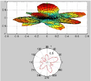
Beamforming experimentation using the Matlab software was performed on the 2x2

array of figure 3.4, the configuration of which is depicted in figure 3.15. The first

experiment was performed using a 1kHz tone located 1.5m from the center of the array at an

azimuth of 90 degrees and an elevation of 0 degrees. The simulated result for this setup is

shown in figure 3.16 which demonstrates both the 3 dimensional and 2 dimensional result.

This is then compared to the real world result of figure 3.17.

(33)

Figure 3.16 Simulated beamforming on 1KHz source at 90 degrees azimuth and no elevation. The result matches the actual location.

(34)

The real world beam pattern maintains a form that is similar to the simulated result

but is obviously noisier, indicative of a less pure tone from the sound source. Realizing that

the testing environment was less than ideal it was surmised that other noise introduced by

several computers, air conditioning, and outside foot and road traffic could be responsible for

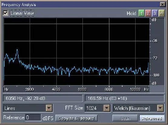
this result. Examining the frequency spectrum of one of the recorded signals shown in figure

3.18 shows that there is a considerable amount of noise lower than the desired 1KHz signal.

Figure 3.18 Frequency spectrum of one of the signals contributing to the beam pattern of figure 3.14.

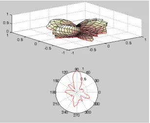
A band-pass filter was introduced in software ranging from 800Hz to 1200Hz to

compensate for the excess noise. As demonstrated in figure 3.19, this produced the desired

result, cleaning up the beam pattern and yielding one more commensurate with the simulated

(35)

Figure 3.19 Real world result after introducing a software filter. Sound source is at 90 degrees azimuth and no elevation. The sound source is detected correctly.

The next simulation is introduced to examine the effect of sound source elevation on

the accuracy of the listening pattern. To do this, the same 1kHz source was used but placed

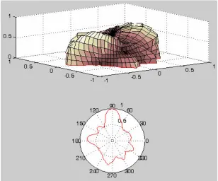
at an azimuth of 90 degrees and elevation of 25 degrees. The resulting beam pattern is

shown in figure 3.20. The detected source is located at an azimuth of 200 degrees and

elevation of 50 degrees, a substantial deviation. Increasing the height of two elements

diagonal to one another yields a non-planar array. Beamforming with the same source at the

same position with this configuration produces the pattern of figure 3.21. The

two-dimensional plot of the beam pattern is misleading as it is a projection of the

three-dimensional plot onto a plane with 0 degrees elevation. The 3 three-dimensional plot has been

oriented to correspond with its two dimensional counterpart. The darker red in this image is

(36)

Figure 3.20 Simulation with sound source located at 90 degrees azimuth and 25 degrees elevation. Detected at an azimuth of 200 degrees and elevation of 50 degrees.

(37)

3.4 Triangulation

A stand-alone demonstrator was developed to triangulate the position of a sound

source. This requires considerably less processing power than beamforming and can

potentially supply distance information as well as direction. The geometrical basis of

triangulation is demonstrated in figure 3.22.

3.4.1 Hardware

The prototype was developed to be a single soldier deployable system. Keeping that

in mind, all of the electronics developed were contained inside of a 3½ft blueprint tube about

which the array itself could be wound. The tube has an LCD display which outputs the

azimuth of the sound source. It also has a serial interface port through which data can be

recorded or the system can be reprogrammed.

d3,1m

d3m d2,1m d2m

θss

θ3

mic 1 (x1,y1) t1

α

β

mic 3 (x3,y3)

t3 mic 2 (x2,y2)

t2

Y

X

d3,1 = distance between mic 3 and

reference mic

θ3,1 = azimuth of the vector from mic 3 to

reference mic

d3,m = calculated distance based on

time delay between mic 3 and reference mic.

θss,3 = bearing of the sound source from

mic 3

(38)

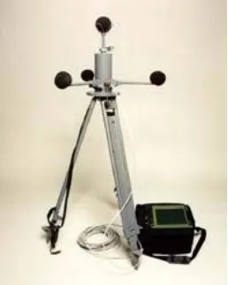
Figure 3.23 Triangulation electronics housed in a blueprint tube.

The electronics were custom designed to record time delays between microphone

elements as a sound impulse propagates across the array. The first microphone to experience

the impulse starts an internal counter. As every microphone hears the sound they latch the

current counter value which is representative of a time delay. A BasicX microprocessor

retrieves this information after all of the microphones have signaled that they have received

the sound. The implemented system is shown in figure 3.23 and a block diagram of this

process is shown in figure 3.24.

(39)

3.4.2 Software

After collecting the counter data and converting it to times based on the speed of

sound, the triangulation method outlined in [43] is applied. This approach uses only four of

the available elements to solve the system of equations shown in figure 3.25. The four corner

microphones are chosen as they are the furthest apart and will provide the largest baseline for

triangulation. Error-checking code was also developed due to occasional aberrations in the

data collected. This code essentially checks the data received from these 4 microphones and

determines whether or not they physically make sense. If not, a neighbor of the erroneous

element is chosen and the calculation is performed.

Figure 3.25 Solving this system of equations yields u (x coordinate of sound source), v (y coordinate of sound source), and d (distance to sound source) where ∆T refers to the time difference between the

microphones designated in the subscripts [43].

3.4.3 Experimentation

To evaluate the performance of the array a sound impulse was generated at various

angles with respect to the center of the array. As long as the impulse was generated at or

near 0 degrees elevation, the results achieved were agreeable to the actual location. Some

error is introduced which can be attributed to the resolution of the counters utilized in the

timing circuitry of the array. If the resolution of the timer is increased, the array should yield

more precise results. Much like the beamforming experimentation, this array is not amenable

(40)

Chapter 4 – System Design

This chapter focuses on the development of the phase II acoustic array system shown

in figure 4.1. This array inherits the polyester substrate and microphones from the previous

array. The areas of concentration are the development of the electrical systems investigated,

the decisions behind the array geometry, the software involved, and an evaluation of the

system’s performance.

(41)

4.1 Electrical Considerations

The electrical aspects of this system are divided into two areas. The first area to

consider is the Mote which is the processing and communications unit of the array. The

second area concerns both the sensors and any signal preprocessing that may be necessary.

This could be a broad topic ranging over several different sensor types, but for the purposes

of this thesis will be limited to the collection, amplification, and filtering of acoustic signals.

4.1.1 The Berkeley Mote Concept

Developed by Jason Hill at the University of California at Berkeley, the mote is a

fully functional microprocessor board centered on the Atmel 90LS8035 microprocessor [44].

This is a 4MHz processor with 32 I/O lines of which 8 can be used as 10-bit analog to digital

converters. It also contains a programmable UART, 512 bytes of SRAM, 512 bytes of

EEPROM, and 8Kb of flash for program storage. The mote is further accentuated with

256Kb of external EEPROM and a 916.5MHz transceiver from RF Monolithics. The entire

device measures only 1.5’’ x 1’’ and is shown in figure 4.2. The mote can function for

several weeks off of two AA batteries if run conservatively. The size and RF capabilities of

the mote are particularly attractive for its inclusion in this system. Since the mote is small it

will minimally affect the flexibility of the host substrate, while the RF transceiver makes it

(42)

Figure 4.2 The Rene mote developed by Jason Hill at UC Berkeley. Top (left), bottom (right)

The mote just described is one of the early generations of mote referred to as the

Rene mote, others being the WES mote and the Mica2 mote, with the latter being the most

functional. The Rene was chosen as it is more powerful than the WES and physically

smaller than the Mica. Initial simulations also suggested that the Rene would be suitable for

beamforming. The Rene mote is shown in figure 4.2 and development information for the

Rene mote can be found in Appendix A.1. Sensor boards have also been developed

including light, temperature, and single channel sound.

Berkeley researchers have also developed software tools for use with the Mote.

TinyOS was developed to allow easy interaction with the components of the mote providing

a platform which can be programmed with a language that is essentially a cross between C

and Java. Also available are TinyDB, which is an SQL database configured to run on the

(43)

4.1.2 Data Acquisition Circuitry

Two different data acquisition circuits were developed for use with the mote. The

first of the proposed systems was designed as a flexible circuit so as to not interfere with

flexibility when included in the textile array. The second system was designed to overcome

shortcomings of the flexible circuit while providing an additional variable gain stage.

4.1.2.1 Flexible Multiplexing Circuit

The first tenet of electronic textiles is that they must maintain the flexibility of their

textile substrate. While electronic components are inherently rigid, advances in component

manufacturing have drastically reduced their size such that they would add little to the

rigidity of a textile system. The problem then is how to provide the appropriate footprint to

connect these components to the fabric in question. To address this issue, a circuit patch

was designed on a Kapton film (developed by Dupont) and then sewn into the target fabric.

The circuit was etched in the Biomedical Microsensors Laboratory (BMMSL) at NCSU and

is shown in figure 4.3. This circuit is designed to contain a multiplexer, an op-amp, a

programmable filter, resistors, capacitors, and connection points for woven wires from the

array.

(44)

The circuit design revolves around the programmable filter which is incorporated to

provide a means for target discrimination in a noisy environment as well as double as an

anti-aliasing filter. It was hoped that by isolating certain frequencies, the array could target

specific vehicles based on identifying frequencies, effectively ignoring other vehicles. The

filter chosen is the MAX263 featuring dual second-order filters, 4 operating modes (band

pass, low pass, high pass, and all pass), 128 possible digitally selected Q values depending on

mode, and a digitally programmable center frequency. It is desirable for all microphones to

use the same device since the filter is relatively expensive and occupies a large amount of

circuit real estate. The microphones were therefore multiplexed using a 74HC4051 analog

mux/demux. This arrangement requires the use of only one of the available analog to digital

converters available on the mote for all eight microphones. To further decrease component

count, the acoustic signals are amplified after the multiplexer. The amplifier is the same 741

op-amp as utilized in the first generation array but is oriented in an inverting configuration

with a gain of 100. The inverting scheme requires fewer external components and reduces

the possibility of undesirable filtering by removing extraneous capacitors. The circuit

diagram and associated bill of materials can be found in Appendix A.4.

Tests on the completed circuit identified a few adverse speed limitations of the

system. The fastest possible sampling time of the mote’s analog to digital converters in the

design used is 154kHz. To simulate simultaneous sampling, all 8 microphones must be

sampled as fast as possible per time step. At 154kHz, each group of eight can sample at a

frequency of 19250Hz. As such however, the time the first microphone is sampled is closer

to the time of the sampling of the last microphone in the previous group than it is to samples

(45)

criterion the maximum frequency which can be sampled is 4812.5Hz. To achieve any

reasonable results however, the target frequency range should be considerably lower. It

would likewise be best to have a larger sampling time between groupings of eight. The small

frequency window left is still suitable for beamforming as most frequencies of military

interest are below 200Hz. This will not however allow the full potential of the filter to be

realized, as it is not a high enough order filter to discriminate among frequencies in this

range. Furthermore, when prototyped, the multiplexer was switched at low speeds and the

chosen signal was passed through both the op-amp and filter, and then analyzed. However,

at high speeds, switching the multiplexer switches the input to the filter. Since the filter is

used primarily as a low pass filter and the input is switched at high frequencies, the input is

essentially nullified.

The multiplexer also has issues with high frequencies. When switching the select

lines on the multiplexer, a small amount of noise is introduced in the output signal.

Amplifying the signals after the multiplexer thereby amplifies the switching noise. Since the

microphone signals have very little amplitude, they are indistinguishable in the amplifier

output. To determine the extent of noise introduced in the signal by the 74LS4051, the least

significant bit of the multiplexer’s select lines was clocked using a function generator while

the other two were grounded. Only microphone 0 was connected to the circuit so the

microphone output should appear only on the low cycle of the lsb clock. The initial test

frequency is 75.69kHz, mimicking the desired switching frequency which is commensurate

with the fastest ADC frequency. Figure 4.4 shows universal acceptance of the signal with

(46)

yielding figure 4.5. Appearance of the signal during the positive cycle of the select clock has

been diminished but noise is still quite significant throughout.

Figure 4.4 Multiplexer crossover of signals occurs

at high frequencies. Top - clock, Bottom - output. Figure 4.5 Multiplexer noise reduces with lower _{frequency but is still prevalent. Top - clock,} Bottom - output.

Another drawback of this design is that it requires a 5V power supply. The mote,

designed to be a low power device, has only a 3V supply. All of the components on the mote

can happily accept a 5V supply, but that would increase the size of an already large battery

pack.

Although proven to not be particularly useful, this is a working circuit and its

flexibility can be demonstrated. The circuit was populated and sewn into a miniature array as

shown in figure 4.6. This system allows the user to specify which microphone to listen to

and will allow filtering of the received signal. While the Kapton based circuit can not be

crumpled or creased, it is a definite advancement in flexibility when compared to a standard

(47)

Figure 4.6 Kapton based circuit sewn into a miniature array.

Figure 4.7 Flexibility demonstration of the Kapton based circuit.

4.1.2.2 Intelligent Variable Gain Data Acquisition System

The data acquisition scheme addressed in this section provides advantages for

distributed arrays working to track the same target. The amplitude of the received target

signal depends on the location of each array with respect to the target sound source. An array

close to the source will have a much higher amplitude than one farther away. While both

(48)

the sound or the closer array could actually saturate. With this in mind, it is desirable to be

able to adjust the amplifier gain based on the sound levels the array detects.

The circuit created is shown in figure 4.8 and the circuit diagram can be found in

appendix A.5. While this acquisition system does not have the flexibility of its predecessor,

its size was minimized to reduce added array rigidity. This board measures approximately

1.4’’x1.8’’ and it is directly pluggable into the mote as well as the array, a re-configurability

feature the flexible array did not have. The array is connected via a flat flex cable and a zero

insertion force connector on the data acquisition board.

Figure 4.8 The 8 channel variable gain data acquisition circuit.

This circuit’s primary component is the LTC6910-2 from Linear Technologies. This

chip is a variable gain op-amp adjustable to gains of 0, 1, 2, 4, 8, 16, 32, and 64 via 3 digital

input lines. This chip alone cannot provide adequate gain for sampling of the microphone

signal, so the incoming signal is first sent to a non-inverting op-amp with a static gain of 100.

(49)

rail-to-rail operation not provided by the standard 741 op-amp used in the previous amplifier

circuitry.

When determining the gain and the possible variable gains it was important to choose

values that would provide high sensitivity without over accentuating ambient noise while at

the same time allowing a target to be located within a few meters of the array without it

saturating. Unfortunately, an anechoic chamber was not readily available and the following

experiments were performed in a typical computer laboratory. To minimize ambient noise,

unnecessary computers were powered down, air conditioning was turned off, and the tests

were run after business hours to avoid people and outside traffic disturbances. The tests were

run utilizing a sound source of 100Hz at 100 decibels (dB). This was chosen as it is the

mid-range of the military vehicle frequency mid-range (20-200Hz) with the dB equivalence of a large

truck or drill. It is important to note that this is dBA which is frequency dependant and

models the sensitivity of the human ear. This is not an appropriate scale for characterization

of this array as it has, as previously shown, a rather consistent frequency response across the

audible range [45]. The dBC scale is therefore utilized for experimentation as it is

independent of frequency. The 100 decibels on the dBA scale has a measured equivalency to

118dBC. Utilizing just the first amplification stage, with a gain of 100, saturation occurs

within 5 meters. This is sufficient for localization such that if an array is saturating and the

array’s position is known, the source position is also known and it can then be targeted.

Initially, two channels of this system were prototyped and tested. The testing showed

that there is little noise introduced on the signals. After fabrication however, the circuit

demonstrated considerable noise. The signal and power lines on the board are in some cases

(50)

make the board as small as possible. It is surmised that this minimization inadvertently

introduced the noise since analog and digital lines run in parallel in close proximity. To

decrease the noise, several approaches were taken. First capacitors were added from power

to ground at each op-amp but showed little benefit. Filtering capacitors were also added at

the output of the op-amp stages also showing no improvement. The coupling capacitor and

pull up resistor for the microphone were removed from the pcb and placed directly on the

back of the microphone, essentially turning it into a three terminal microphone. The power is

therefore run separately from the ground and signal wires which are a twisted pair. This

showed promise but still did not yield the desired results. When completed the alterations

allowed for acceptable performance on only 4 of the 8 channels whereas initially only 2 were

usable.

Although the fabricated circuit is not functional enough to be useful, the circuit

design is still viable. The circuit was therefore prototyped on a standard breadboard and

interfaced to the acoustic array until a new layout could be fabricated. This prototype only

contains the first gain stage (the LT1807) simply for testing purposes (figure 4.9).

(51)

4.2 Array Geometry

The second-generation system also attempts to improve performance by altering the

microphone geometry. During simulation with the 4 x 5 element array of figure 3.1, whose

layout is shown in the plot of figure 4.10, system ambiguity was observed when the sound

source was perpendicular to the broad side of the array or at 90 degrees with reference to the

array’s center. This is shown with the spurious spikes in the leftmost image of figure 4.11.

Also shown in this figure is a simulation with the sound source located at 0 degrees. In this

orientation, there is one obvious directional beam with only insignificant extraneous beams.

(52)

Figure 4.11 Beam Forming Simulations for the Rectangular Array of figure 4.10. Multiple beams are observed with a 1kHz sound source at 90 degrees (left) but are not present when located at 0 degrees (right).

The new array layout attempts to obtain a more consistent beam pattern regardless of

the position of the sound source. This would help to eliminate any confusion caused by

spurious beams as demonstrated. To accomplish this, the array was laid out in a circular

pattern. Furthermore, it was laid out such that there are 7 elements along the perimeter and

one in the center (only 8 are used as there are only 8 ADC ports available on the mote). The

simulations of figure 4.13 show that the acoustic array geometry as proposed gives more

consistent results and is less likely to introduce confusion. Although there are many

extraneous spikes in the diagrams, it is important to realize that a longer spike equates to

higher confidence, so these particular spikes do not carry as much weight as those in the

rectangular simulation at 90 degrees. With the maximum distance between microphones of

approximately 1 meter, this array is best suited for frequencies greater than 350Hz. For

better performance at lower frequencies a much larger array would be needed. For example,

minimal spacing for detection of a 20Hz signal is 17.25m and for 100Hz is 3.45m. These

would be more ideal for beam-forming with military targets (characteristically 20-200Hz) but

(53)

Figure 4.12 8 element array configuration for mote based sensing.

Figure 4.13 Beam Forming Simulations of 8 Element Circular Array at 0, 45, and 90 degrees Respectively given a 1kHz sound source.

4.3 Software

The software involved is responsible for the control of the data acquisition, the

communication between motes or base computer, and processing of the data for

(54)

from the base node and then transmit that information back to the base node for processing.

This can be done either directly through the serial port or through an intermediary mote

which essentially serves to provide RF capabilities to a PC. To facilitate the RF operation, a

board was created based on the mote programmer of Appendix A.2 that simply performs

RS232 communication. The layout for this board can be found in Appendix A.3. The home

computer then must process the information gathered and present it to the user.

4.3.1 Data Acquisition Software

The data acquisition software is largely dependant upon the hardware components

available on the mote. Data must not only be sampled and stored at an appropriate

frequency, to sample the target acoustic source, but each of the eight channels must be

sampled fast enough that the sampling delay between channels can be considered negligible.

Due to the stringent timing requirements of this program, it was coded in assembly.

As previously outlined, the mote has three types of memory: 512 bytes of internal

SRAM, 512 bytes of internal EEPROM, and 256Kb of external EEPROM. Ideally the

external EEPROM would be utilized, as it would allow for a considerable amount of

sampling of the target signal. This memory is serial and accessed via the I2C protocol.

While this does not require much of the processor’s resources, it is regrettably slow with a

maximum write time of 5.0ms. While faster, the internal EEPROM is also too slow due to its

large write time of 2.5-4.0ms. The SRAM is the only viable solution as it can be written to in

two clock cycles (0.5µs) but it is important to note that the data must share its meager 512

bytes with the program stack. Fortunately, the software on the array does not require

(55)

bytes available for data. The analog to digital converter output on the mote has a 10 bit

resolution, requiring 2 bytes of storage per sample. This would allow for only 31 samples

which is insufficient, so the data is left aligned to ignore the lower 2 bits thereby allowing for

62 samples per microphone.

Ideally, all eight channels would be sampled simultaneously. The mote’s ADCs do

not sample simultaneously so it is necessary to sample all eight channels as fast as possible to

make the timing difference appear negligible. Using the ADC in free running mode and the

maximum 2MHz ADC clock (given a 4MHz system clock), samples are taken at

approximately 154k samples per second. The eight samples at 154kHz in this example are

only taken every 640Hz so a software timer must be introduced to meet this requirement.

Timer Counter 0 is set up for this purpose. This timer uses the system clock (4Mhz),

prescaled by a factor of 32, or 125kHz (otherwise the count necessary would be larger than 1

byte). At this frequency, if the counter counts to 195 every 1.5625ms for a frequency of

640Hz. After 8 ADC samples, the ADC is disabled. After Timer Counter 0 counts to 195,

the counter is reset and the ADC is enabled. The timing associated with the ADC and Timer

(56)

Figure 4.14 Oscilloscope screen shot displaying the sampling frequency used to sample the acoustic source (top) and the sampling time used to sample the 8 microphone elements (bottom).

The main program as shown in the flowchart of figure 4.15 primarily serves to

initialize the system for data collection and to communicate with the base station. The

program first awaits a start signal from the base computer (or polls the RF receiver)

instructing it to begin sampling. Once received, the necessary hardware is initialized and the

interrupts are enabled. The ADC and OC2 interrupts perform the sampling operation until

the SRAM is full then stop collecting data. Control is returned to the main program which

transmits the collected data (either through the UART or the RF transceiver). The program

(57)