ABSTRACT
REIMANN, CRAIG AARON. Development of a General Methodology for Optimizing Acoustic Treatment using an Equivalent Source Method. (Under the direction of Dr. Robert Nagel.)
Development of a General Methodology for Optimizing Acoustic Treatment using an Equivalent Source Method
by
Craig Aaron Reimann
A dissertation submitted to the Graduate Faculty of North Carolina State University
in partial fulfillment of the requirements for the Degree of
Doctor of Philosophy
Aerospace Engineering
Raleigh, NC
2007
APPROVED BY:
________________________________ ________________________________ Dr. Ashok Gopalarathnam Dr. Terry Scharton
Advisory Committee Member Advisory Committee Member
________________________________ ________________________________ Dr. Harvey Charlton Dr. Robert Nagel
BIOGRAPHY
ACKNOWLEDGMENTS
I would first like to thank my family for their continuous support. I would like to thank my fiancé for being there for me. While in Virginia, I had the opportunity to make a lot of new friends, so I would like to thank them for helping make this a great experience.
TABLE OF CONTENTS
List of Tables...vi
List of Figures ...vii
List of Symbols ...xi
1. Background ...1
1.1 Community Noise Problem...1
1.2 Liner Technology...2
1.3 Computational Efforts in Aeroacoustics ...5
1.3.1 Finite Element Method (FEM)...7
1.3.2 Finite Volume Method (FVM)...9
1.3.3 Boundary Element Method (BEM)...10
1.3.4 Equivalent Source Method (ESM)...13
1.4 Motivation and Challenges...15
1.5 Objectives...16
2. Computational Tool – Fast Scattering Code ...18
2.1 Introduction...18
2.2 FSC Methodology...19
2.3 Uses/Examples of FSC ...24
3. Validation of Sound Absorbent Boundary Condition...27
3.1 Introduction...27
3.2 Point Source above an Impedance Boundary ...27
3.2.1 Test Cases ...31
3.2.2 Results...31
3.3 Conclusions...38
4. Optimization Methods ...39
4.1 Introduction...39
4.2 Contour Method (CtrMd) ...43
4.3 Powell...44
4.4 Broyden-Fletcher-Goldfarb-Shanno (BFGS) ...45
4.5 Stewart-Davidon-Fletcher-Powell (SDFP) ...47
4.6 Stochastic-Integration Global Minimization Algorithm (SIGMA)...47
4.7 Genetic Algorithm (GA)...48
5. Results & Discussion ...50
5.1 Commercial Transport Nacelle ...50
5.1.1 Inlet Liner ...51
5.1.2 Exit Liner ...56
5.2 Duct Acoustics and Mode Generation ...66
5.3 Liner Impedance Optimization for a Rectangular Duct ...69
5.4 Liner Impedance Eduction for a Rectangular Duct ...72
6. Conclusions ...76
7. References ...79
8. Tables ...91
9. Figures...102
10. Appendices...156
10.1 Zero Finding Method for the Eigenvalue Problem of Soft-Wall Rectangular Duct ....156
LIST OF TABLES
Table 5.1 - Inlet Liner results from all optimization methods. n = 2,
M = 0.0, 2xBPF, m = -10. ...91
Table 5.2 - Inlet Liner results from all optimization methods. n = 2,
M = 0.2, 2xBPF, m = -10. ...92 Table 5.3 - Inlet Liner results from all optimization methods. n = 4,
M = 0.0, 2xBPF, m = -10. ...92
Table 5.4 - Inlet Liner results from all optimization methods. n = 4,
M = 0.2, 2xBPF, m = -10. ...93
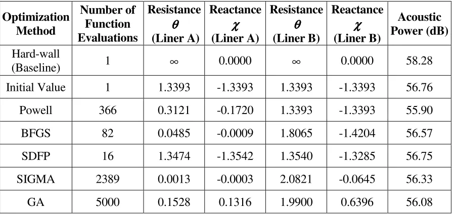
Table 5.5 - Exit Liner results from all optimization methods. n = 2,
M = 0.0, 2xBPF, m = -10. ...93
Table 5.6 - Exit Liner results from all optimization methods. n = 2,
M = 0.2, 2xBPF, m = -10. ...94
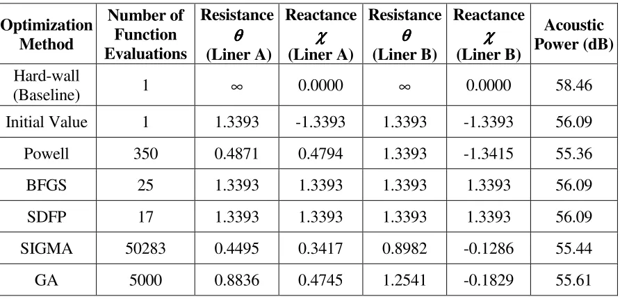
Table 5.7 - Exit Liner results from all optimization methods. n = 4,
M = 0.0, 2xBPF, m = -10. ...94 Table 5.8 - Exit Liner results from all optimization methods. n = 4,
M = 0.2, 2xBPF, m = -10. ...95
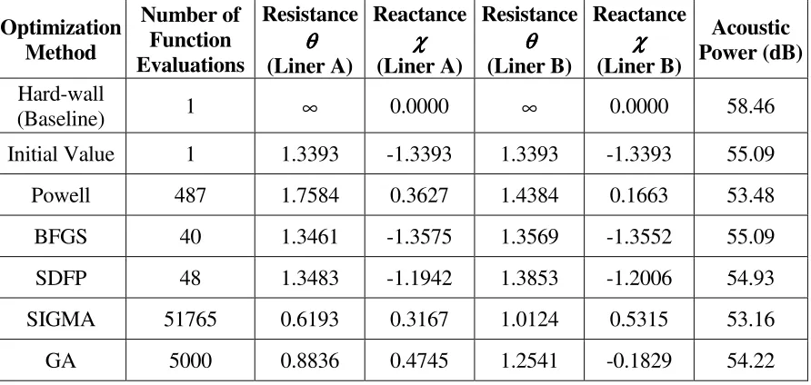
Table 5.9 - Inlet and Exit Liners results from all optimization methods. n = 2,
M = 0.0, 2xBPF, m = -10. ...95
Table 5.10 - Inlet and Exit Liners results from all optimization methods. n = 2,
M = 0.2, 2xBPF, m = -10...96
Table 5.11 - Inlet and Exit Liners results from all optimization methods. n = 4,
M = 0.0, 2xBPF, m = -10...96
Table 5.12 - Inlet and Exit Liners results from all optimization methods. n = 4,
M = 0.2, 2xBPF, m = -10...97 Table 5.13 - Inlet and Exit Liners results from all optimization methods.
n = 8, M = 0.0, 2xBPF, m = -10. ...98
Table 5.14 - Inlet and Exit Liners results from all optimization methods.
n = 8, M = 0.2, 2xBPF, m = -10. ...98
Table 5.15 - Inlet and Exit Liners results from all optimization methods. n = 4,
M = 0.0, 3xBPF, m = 12. ...99
Table 5.16 - Inlet and Exit Liners results from all optimization methods. n = 4,
M = 0.2, 3xBPF, m = 12. ...99
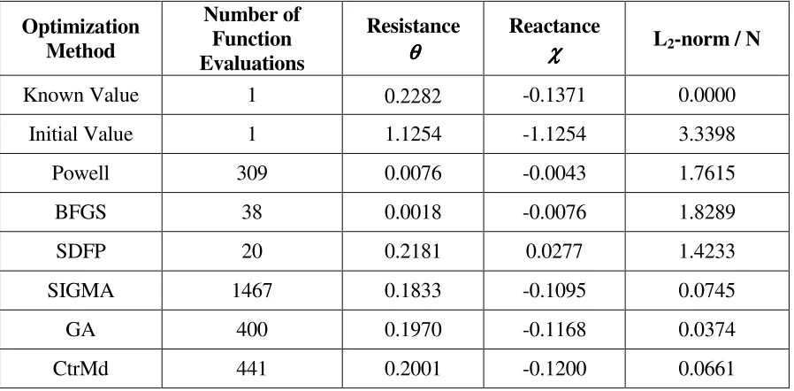
Table 5.17 - Rectangular duct results from all optimization methods.
M = 0.0, f = 1500Hz, and dominant (0,0) mode. ...100 Table 5.18 - Rectangular duct eduction results for soft-wall from all optimization
methods. M = 0.0, f = 1500Hz, and dominant (0,0) mode. ...100
Table 5.19 - Rectangular duct eduction results for hard-wall from two optimization
methods. M = 0.0, f = 1500Hz, and dominant (0,0) mode. ...101
Table 10.1 - Eigenvalues (Zeros) for infinitely long rectangular duct
with acoustic treatment. M = 0.0, f = 1500Hz, (0,0) mode,
LIST OF FIGURES
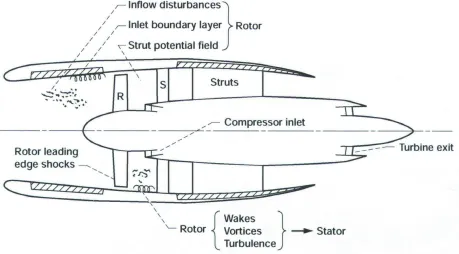
Figure 1.1 - Noise Sources for Turbofan Engine. (Ref. 2). ...102
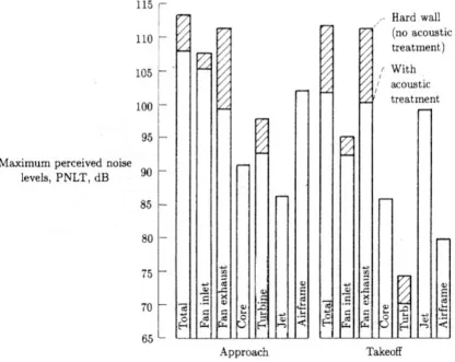
Figure 1.2 - Noise Components for turbofan engine. (Ref. 1)...103
Figure 1.3 - Acoustic treatment design parameters. a) SDOF, b) 2DOF, and c) Bulk Absorber. (Ref. 5)...104
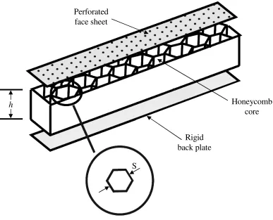
Figure 1.4 - Acoustic treatment schematic. (Ref. 34). ...105
Figure 2.1 - Predefined geometry in uniform motion. (Ref. 61). ...105
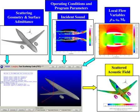
Figure 2.2 - Main dialog screen for the FSC GUI. (Ref. 72)...106
Figure 2.3 - Sound pressure levels on the surface of a commercial transport vehicle. M = 0.0, f = 3 kHz. a) Top Surface and b) Bottom Surface. (Ref. 61). ...107
Figure 2.4 - Noise footprints for model commercial transport during take-off. M = 0.2, f = 3kHz, climb angle = 22.5o. (Ref. 61)...108
Figure 2.5 - Acoustic pressure contours in the vicinity of a 2.68% scale model of a commercial transport. M = 0.2, f = 5 kHz, m = 2 (sources spinning in the same direction). (Ref. 70)...109
Figure 2.6 - Mode propagation within a sinusoidal test section with hard-walls. M = 0.0, f = 1500 Hz, dominant (0, 0) mode. (Ref. 67). ...110
Figure 3.1 - Acoustic point source above a boundary. (Ref. 94)...111
Figure 3.2 - Incident acoustic pressure field for a point source. M = 0.0, f = 100Hz. a) Analytical and b) FSC...112
Figure 3.3 - Incident acoustic pressure field for a point source. M = 0.3, f = 100Hz. a) Analytical and b) FSC...112
Figure 3.4 - Plot of the incident acoustic pressure at an observer x-location for a point source at x = 10m. M = 0.0, f = 100Hz. x = a) 0.2m and b) 10m. ...113
Figure 3.5 - Plot of the incident acoustic pressure at an observer x-location for a point source at x = 10m. M = 0.3, f = 100Hz. x = a) 0.2m and b) 10m...113
Figure 3.6 - Acoustic pressure field for a point source 1m above a hard-wall boundary. M = 0.0, f = 75Hz. a) Analytical and b) FSC...114
Figure 3.7 - Acoustic pressure field for a point source 1m above a hard-wall boundary. M = 0.0, f = 100Hz. a) Analytical and b) FSC...114
Figure 3.8 - Acoustic pressure field for a point source 1m above a hard-wall boundary. M = 0.0, f = 125Hz. a) Analytical and b) FSC...114
Figure 3.9 - Acoustic pressure field for a point source 1m above a soft-wall boundary. M = 0.0, f = 75Hz. a) Analytical and b) FSC...115
Figure 3.10 - Acoustic pressure field for a point source 1m above a soft-wall boundary. M = 0.0, f = 100Hz. a) Analytical and b) FSC. ...115
Figure 3.11 - Acoustic pressure field for a point source 1m above a soft-wall boundary. M = 0.0, f = 125Hz. a) Analytical and b) FSC. ...115
Figure 3.12 - Acoustic pressure field for a point source 1m above a hard-wall boundary. M = 0.3, f = 75Hz. a) Analytical and b) FSC. ...116
Figure 3.14 - Acoustic pressure field for a point source 1m above a hard-wall boundary.
M = 0.3, f = 125Hz. a) Analytical and b) FSC. ...116
Figure 3.15 - Acoustic pressure field for a point source 1m above a soft-wall boundary. M = 0.3, f = 75Hz. a) Analytical and b) FSC. ...117
Figure 3.16 - Acoustic pressure field for a point source 1m above a soft-wall boundary.
M = 0.3, f = 100Hz. a) Analytical and b) FSC. ...117 Figure 3.17 - Acoustic pressure field for a point source 1m above a soft-wall boundary.
M = 0.3, f = 125Hz. a) Analytical and b) FSC. ...117
Figure 3.18 - Acoustic pressure field for a point source 10m above a hard-wall boundary.
M = 0.0, f = 75Hz. a) Analytical and b) FSC. ...118
Figure 3.19 - Acoustic pressure field for a point source 10m above a hard-wall boundary.
M = 0.0, f = 100Hz. a) Analytical and b) FSC. ...118
Figure 3.20 - Acoustic pressure field for a point source 10m above a hard-wall boundary. M = 0.0, f = 125Hz. a) Analytical and b) FSC. ...118
Figure 3.21 - Acoustic pressure field for a point source 10m above a soft-wall boundary.
M = 0.0, f = 75Hz. a) Analytical and b) FSC. ...119 Figure 3.22 - Acoustic pressure field for a point source 10m above a soft-wall boundary.
M = 0.0, f = 100Hz. a) Analytical and b) FSC. ...119
Figure 3.23 - Acoustic pressure field for a point source 10m above a soft-wall boundary.
M = 0.0, f = 125Hz. a) Analytical and b) FSC. ...119
Figure 3.24 - Acoustic pressure field for a point source 10m above a hard-wall boundary.
M = 0.3, f = 75Hz. a) Analytical and b) FSC. ...120
Figure 3.25 - Acoustic pressure field for a point source 10m above a hard-wall boundary. M = 0.3, f = 100Hz. a) Analytical and b) FSC. ...120
Figure 3.26 - Acoustic pressure field for a point source 10m above a hard-wall boundary.
M = 0.3, f = 125Hz. a) Analytical and b) FSC. ...120 Figure 3.27 - Acoustic pressure field for a point source 10m above a soft-wall boundary.
M = 0.3, f = 75Hz. a) Analytical and b) FSC. ...121
Figure 3.28 - Acoustic pressure field for a point source 10m above a soft-wall boundary.
M = 0.3, f = 100Hz. a) Analytical and b) FSC. ...121
Figure 3.29 - Acoustic pressure field for a point source 10m above a soft-wall boundary.
M = 0.3, f = 125Hz. a) Analytical and b) FSC. ...121
Figure 3.30 - Plot of the acoustic pressure at a height of 0.2m for a point source above a hard-wall boundary. M = 0.0, f = 75Hz. a) 1m and b) 10m. ...122
Figure 3.31 - Plot of the acoustic pressure at a height of 0.2m for a point source above
a hard-wall boundary. M = 0.0, f = 100Hz. a) 1m and b) 10m. ...122 Figure 3.32 - Plot of the acoustic pressure at a height of 0.2m for a point source above
a hard-wall boundary. M = 0.0, f = 125Hz. a) 1m and b) 10m. ...122
Figure 3.33 - Plot of the acoustic pressure at a height of 0.2m for a point source above
a soft-wall boundary. M = 0.0, f = 75Hz. a) 1m and b) 10m. ...123
Figure 3.34 - Plot of the acoustic pressure at a height of 0.2m for a point source above
a soft-wall boundary. M = 0.0, f = 100Hz. a) 1m and b) 10m. ...123
Figure 3.36 - Plot of the acoustic pressure at a height of 0.2m for a point source above
a hard-wall boundary. M = 0.3, f = 75Hz. a) 1m and b) 10m. ...124
Figure 3.37 - Plot of the acoustic pressure at a height of 0.2m for a point source above a hard-wall boundary. M = 0.3, f = 100Hz. a) 1m and b) 10m. ...124
Figure 3.38 - Plot of the acoustic pressure at a height of 0.2m for a point source above a hard-wall boundary. M = 0.3, f = 125Hz. a) 1m and b) 10m. ...124
Figure 3.39 - Plot of the acoustic pressure at a height of 0.2m for a point source above a soft-wall boundary. M = 0.3, f = 75Hz. a) 1m and b) 10m. ...125
Figure 3.40 - Plot of the acoustic pressure at a height of 0.2m for a point source above a soft-wall boundary. M = 0.3, f = 100Hz. a) 1m and b) 10m. ...125
Figure 3.41 - Plot of the acoustic pressure at a height of 0.2m for a point source above a soft-wall boundary. M = 0.3, f = 125Hz. a) 1m and b) 10m. ...125
Figure 3.42 - Plot of the scattered acoustic pressure at a height of 0.2m for a point source 10m above a boundary. M = 0.0, f = 100Hz. a) hard-wall and b) soft-wall. ...126
Figure 3.43 - Plot of the scattered acoustic pressure at a height of 0.2m for a point source 10m above a boundary. M = 0.3, f = 100Hz. a) hard-wall and b) soft-wall. ...126
Figure 4.1 - GE90 engine and nacelle schematic. (Ref. 70). ...127
Figure 4.2 - Relative placement of nacelle with arc. ...128
Figure 4.3 - Nacelle liner configurations. a) Inlet n = 2, b) Inlet n = 4, c) Exit n = 2, d) Exit n = 4, e) Inlet and Exit n = 2, f) Inlet and Exit n = 4, and g) Inlet and Exit n = 8...129
Figure 4.4 - The optimization process...130
Figure 4.5 - Convergence of Powell’s method with conjugate directions. (Ref. 99)...131
Figure 4.6 - Convergence of Powell’s method without conjugate direction-sets. ...132
Figure 4.7 - Convergence of Gradient-Based method. ...133
Figure 5.1 - Equivalent source placement for GE90-type Nacelle...134
Figure 5.2 - Contour plot to obtain minimum specific impedance for the Inlet Liner configuration. 2xBPF, m = -10, a) M = 0.0 and b) M = 0.2...135
Figure 5.3 - Sound Pressure Level field for a GE90-type nacelle with Inlet Liner. M = 0.0, 2xBPF, m = -10. a) Hard-wall, b) Optimized Liner (n = 2), and c) Optimized Liner (n = 4). ...136
Figure 5.4 - Sound Pressure Level field for a GE90-type nacelle with Inlet Liner. M = 0.2, 2xBPF, m = -10. a) Hard-wall, b) Optimized Liner (n = 2), and c) Optimized Liner (n = 4). ...137
Figure 5.5 - Contour plot to obtain minimum specific impedance for the Exit Liner configuration. 2xBPF, m = -10, a) M = 0.0 and b) M = 0.2...138
Figure 5.6 - Sound pressure level field for a GE90-type nacelle with Exit Liner. M = 0.0, 2xBPF, m = -10. a) Optimized Liner (n = 2) and b) Optimized Liner (n = 4)...139
Figure 5.8 - Contour plot to obtain minimum specific impedance for the Inlet and Exit Liner configuration. 2xBPF, m = -10, a) M = 0.0 and b) M = 0.2. ...141
Figure 5.9 - Sound Pressure Level field for a GE90-type nacelle with Inlet and Exit Liner. M = 0.0, 2xBPF, m = -10. a) Optimized Liner (n = 2), b) Optimized
Liner (n = 4), and c) Optimized Liner (n = 8). ...142
Figure 5.10 - Sound Pressure Level field for a GE90-type nacelle with Inlet and Exit Liner. M = 0.2, 2xBPF, m = -10. a) Optimized Liner (n = 2), b) Optimized
Liner (n = 4), and c) Optimized Liner (n = 8). ...143
Figure 5.11 - Sound Pressure Level field for a GE90-type nacelle with Inlet and Exit Liner. M = 0.0, 3xBPF, m = 12. a) Hard-wall and b) Optimized
Liner (n = 4). ...144
Figure 5.12 - Sound Pressure Level field for a GE90-type nacelle with Inlet and Exit Liner. M = 0.2, 3xBPF, m = 12. a) Hard-wall and b) Optimized Liner (n = 4)...145
Figure 5.13 - Noise generation process of turbomachinery. (Ref. 1). ...146 Figure 5.14 - Schematic of rectangular duct with acoustic treatment in red...147 Figure 5.15 - Acoustic Pressure field along the y = 0.0 m plane for a hard-wall duct.
M = 0.0, f = 1500Hz, and dominant (0,0) mode a) Analytical
(Appendix 10.1) and b) FSC. ...148 Figure 5.16 - Schematic of rectangular duct with optimization planes at the In (blue)
and Out (yellow) locations. ...149 Figure 5.17 - Contour plot to obtain maximum ∆dB. M = 0.0, f = 1500Hz, and
dominant (0,0) mode. ...150 Figure 5.18 - Acoustic Pressure field along the y = 0.0 m plane for a soft-wall duct
(ζopt = 0.8921 - 0.4393i). M = 0.0, f = 1500Hz, and dominant (0,0) mode. .151
Figure 5.19 - Schematic of rectangular duct with acoustic treatment (in red) and
measured/calculated acoustic pressure field (in blue) locations. ...151 Figure 5.20 - Contour plot to obtain minimum L2-norm / N. M = 0.0, f = 1500Hz, and
dominant (0,0) mode. ...152 Figure 5.21 - Acoustic Pressure field along the x = 0.4064 m plane for two impedance
values. Soft-wall, M = 0.0, f = 1500Hz, and dominant (0,0) mode.
a) known and b) educed (GA)...153 Figure 5.22 - Acoustic Pressure field along the x = 0.4064 m plane for two impedance
values. Hard-wall, M = 0.0, f = 1500Hz, and dominant (0,0) mode.
a) known and b) educed (Powell). ...154 Figure 10.1 - Side and front view of 3-D Rectangular Duct geometry and coordinate
system. ...169 Figure 10.2 - Rectangular duct mode patterns for a hard-wall duct. m = 0, 1, 2 and
n = 0, 1, 2. ...169
LIST OF SYMBOLS Roman Symbols
a Source strength, lower limit, pressure coefficient
A Complex acoustic admittance
b Upper limit and velocity coefficient
B Source strength (γ2
/4π) and number of rotor blades
B Modified identity matrix
c Speed of sound
C “White noise” terms and unknown source density d Distance between hard-wall and acoustic treatment F Boundary-loss factor and functional
h Step length
H Duct height
I Identity matrix
k mode number and wave number
m Mode order
M Mach number
Ns Number of equivalent sources
P Unknown variable
Pj Simple sources
q Source function
Q Image source strength, collection of sources, area of sources
R Distance between two points, radius, acoustic resistance, and flux terms
Rp Plane wave reflection coefficient
S Scattering geometry and direction-set
T Transformed time (Lorentz)
V Number of stator vanes
W Duct width
X Transformed Cartesian coordinate and acoustic reactance
Y Transformed Cartesian coordinate
Z Transformed Cartesian coordinate and complex acoustic impedance f Source excitation frequency and objective function
F Numerical flux
i Imaginary unit ( −1) and index number
j Number of uniform liners in the engine nacelle configuration and index
number
m Number of sides of an element
n Surface Normal and index number
nˆ Unit surface normal
nn Total number of nodes
Ns Total number of sides of an element
p Pressure
r Arc radius
S Scattering geometry, surface area, and domain
t Original time
Tγ Retarded time
u Velocity and acoustic pressure/velocity
v Velocity
V Volume area
x Original Cartesian coordinate
y Original Cartesian coordinate
z Original Cartesian coordinate
Greek Symbols
α Mode number (πy/H)
β Mach number relation ( 1 2
M
− )
χ Specific acoustic reactance
φ Angle of incidence
γ Lorentz factor and adiabatic index
κ Modified wave number ( k / β)
λ Wavelength and step length
µ Mode number (πz/W) and harmonic
π 3.14159…
θ Specific acoustic resistance
ρ Density
τ Transformed time variable (Galilean)
ω Excitation frequency
ωd Numerical distance
ξ New independent variable
ψ Shape function
ζ Specific acoustic impedance
Subscripts
a Axial
γ Function of the Lorentz factor
0 Background flow
1 New dependent variable and distance from source to observer
2 Distance from image to observer
s Scattered field
in Start of acoustic treatment
inc Incident field
kwn Known values
out End of acoustic treatment
ξ In terms of new independent variable ξ
Superscripts
* Complex conjugate
+ Exterior to scattering geometry
' Acoustic variable
→ Vector
∧ Non-dimensional value
Abbreviations
BFGS Broyden-Fletcher-Goldfarb-Shanno
CtrMd Contour Method
CDTR Curved Duct Test Rig
ESM Equivalent Source Method
FEM Finite Element Method
FSC Fast Scattering Code
FVM Finite Volume Method
GA Genetic Algorithm
LaRC Langley Research Center
NASA National Aeronautics and Space Administration NIA National Institute of Aerospace
NCSU North Carolina State University SDFP Stewart-Davidon-Fletcher-Powell
SIGMA Stochastic-Integration Global Minimization Algorithm
Units of Measurement
dB Decibel
Hz Hertz
Pa Pascal
s second
Miscellaneous Symbols
| | Absolute value
∂ Partial derivative
∈ Is an element
[ ]
d Derivative
• Dot product
d/dt Time derivative of a quantity
! Factorial
∇ Gradient
∇2 Laplacian
∞ Infinity
Im( ) Imaginary part
[ ]
∫
IntegralO( ) Of the order
Re( ) Real part
C h a p t e r 1
BACKGROUND 1.1 Community Noise Problem
The unprecedented growth in air traffic over the last two decades, coupled with urban expansion, has made community noise a serious problem in many cities around the world. The environmental concerns associated with this noise problem, along with the need to accommodate increasing passenger and cargo loads without compromising the aircraft’s fuel efficiency and aerodynamic performance, while minimizing the need for changes to existing airport infrastructure and operations, are some of the most important factors driving the design of modern aircraft.
potential benefits of liners abound in the open literature,5 continually advancing the state of the art in acoustic liner design.
1.2 Liner Technology
The use of acoustic liner treatment dates back to the 1960s and continues to be explored as a possible means of reducing engine noise (fan noise in particular). The problem that exists stems from the frequency dependency of acoustic treatment and its required bandwidth. Fan noise in the form of tonal noise based on the Blade Passage Frequency (BPF), varies for the different operating conditions (takeoff and approach), thus making it difficult to design acoustic treatment with a large enough bandwidth to capture the frequencies of interest for the entire range of operating conditions. Ideally, a single acoustic treatment could handle all operating conditions, but this in not the case. Thus, three common acoustic treatment type designs include: single degree of freedom (SDOF), two degree of freedom (2DOF), and the bulk absorber (see Figure 1.3).5 The SDOF and 2DOF are both based upon the Helmholtz resonator.
construction: solid back plate, fibrous/porous mat center, and porous face sheet. The three designs are presented in order of increasing frequency bandwidth.
Although the three acoustic treatment designs vary in construction, they each are designed to have a particular impedance value. Impedance is the property that is most commonly used to define an acoustic treatment. For a harmonic source (eiωt), impedance is defined as:
iX R
Z = + (1.1)
where R is the resistance and X is the reactance at a point on the acoustic treatment surface. If the impedance value at that point is not affected by neighboring points, then the surface is called a locally reacting surface. If each point affects the other, then the surface is called extended reaction. Impedance values can be achieved by different approaches because the resistance and reactance are functions of the acoustic treatment design.
For the SDOF design, the resistance will remain relatively constant with frequency for a linear face, achieved by having very fine mesh of holes in the face sheet. A face sheet that has a nonlinear frequency behavior in a no flow environment can be forced to behave as a linear face sheet by introducing a mean flow. However, nonlinear resistance peaks may exist near frequencies where the reactance approaches zero. The reactance of a single-layer design follows a modified cotangent curve, such that the most effective impedance value (gives greatest noise reduction) is obtained at a single frequency.
important roles in defining the impedance of the acoustic treatment. First, it controls the resistance of the acoustic treatment surface versus the face sheet, making the acoustic treatment properties independent of duct flow effects. Second, it allows for the resistance and reactance to be tailored towards the desired design values over a larger range of frequencies (as compared to the SDOF).
The third acoustic treatment design (bulk absorber) has a few advantages over the 2DOF design: (1) the resistance of the bulk absorber is distributed continuously over the acoustic treatment depth while the 2DOF is a combination of the face sheet and septum, (2) The fibrous mat can be designed to vary the amount of internal flow resistance based on mat density and fiber diameter, and (3) the desired minimum tuning frequencies can be achieved with slightly thinner acoustic treatment depths as compared to resonator3 types, due to viscous and heat transfer effects of the fibrous mat. Although the bulk absorber provides the largest frequency bandwidth, extra weight introduced by the fibrous mat becomes an issue when considering incorporating onto an aircraft engine nacelle.
1.3 Computational Efforts in Aeroacoustics
As researchers continue to explore methods of reducing noise from aircraft, advances in computer technology have facilitated a substantial growth in computational efforts aimed at predicting/simulating the physical mechanisms that produce noise.7, 8, 9, 10, 11 Because of their lower cost, relative to experimental investigations, numerical studies12, 13, 14 are becoming the preferred approach for analyzing configuration and parameter changes during the preliminary stages of next-generation aircraft and engine liner designs.
The simulation of aerodynamically generated noise can be performed using several approaches. In order of decreasing computational intensity, these are: Computational Aeroacoustics (CAA),15, 16, 17, 18, 19, 20 hybrid methods,21 integral acoustic models, 22, 23, 24, 25, 26 and boundary models.27
The most accurate and comprehensive way to simulate aerodynamic sound is CAA, which is a time-dependent simulation of the entire fluid region, encompassing the noise sources, receivers, and the transmission path. Through a rigorous calculation of the transient flow structures, pressure disturbances in the source regions can be identified and tracked. Sound transmission is simulated by resolving the pressure waves traveling through the fluid. Because of the high computational demands of CAA, this approach can be applied only to relatively small regions of interest in which the sources and observers (receivers) are in close proximity, and the sound to be simulated is of low frequency and fairly high amplitude.
properly resolve the acoustic sources; sound transmission is simulated using a wave equation solver to propagate the sound waves to the far field.
The approach of solving the flow and sound fields separately can be further simplified if the observer has an unobstructed view of the sources, i.e., there exists a straight propagation path. In such cases, sound transmission can be simulated using analytical formulations. Such integral approaches are based on the Lighthill Acoustic Analogy.28, 29 The Ffowcs-Williams and Hawkings method,30 which extends the analogy to cases where the sound source is a solid, permeable, or rotating surface, is the most widely used of the integral acoustic models.
desired form, the domain is then discretized by subdividing the physical space/domain into elements. This may be carried out on and around, or just on, the boundaries, depending on the method chosen to solve the acoustic equations. How the domain is subdivided and where the governing equations are specified within the domain is discussed in the following subsections. Four of the more common methods used today to solve the linearized differential equations relevant to acoustics are briefly introduced: Finite Element Method (FEM), Finite Volume Method (FVM), Boundary Element Method (BEM), and Equivalent Source Method (ESM). 1.3.1 Finite Element Method (FEM)
The Finite Element Method dates back to the 1950s.31 The FEM is based on the idea of building blocks or finite elements that are created to represent the geometry (wing, engine, and/or duct) and domain of interest. The physics of the problem are captured by the use of a set of governing differential equations. The equations are prescribed for each element (typically at element nodes), which are grouped to form sets of matrices that can be solved by linear algebra techniques.
form a volumetric shape) has unknown variables that vary in all three directions. These finite elements are created by subdividing the geometry and field of interest.
No matter how the geometry or field is subdivided, the basic idea behind the FEM is to minimize an energy functional, consisting of all the energies associated with the finite element model, which satisfies the law of conservation of energy. The minimum is found by taking the derivative and setting it equal to zero, thus, the basic equation for finite element analysis is
0 = ∂ ∂ p F
(1.2)
where F is the functional and p is the unknown variables of interest (acoustic pressure or velocity) at the grid points. Geometric functions to approximate the unknown variables of interest are called shape functions. The shape functions range from first-order to high-order polynomials. The higher the order, the more grid points are required to solve for all the polynomial coefficients. A particular type of finite element that contains shape functions that conform to the shape of the element is called an isoparametric finite element.31
matrices. Note, for the FEM the matrix to be inverted is typically sparse (contains zeros), which slightly simplifies the problem.32
This method has been extensively used in acoustics to investigate problems pertaining to liners,33,34,35,36 duct propagation,37 and interior acoustics.38 The FEM has one main drawback, which will become clearer in the upcoming sections, it is limited to finite domains, such as interior type problems.
1.3.2 Finite Volume Method (FVM)
The Finite Volume Method is similar to the FEM, but instead of using the finite element grid points, the area (2-D) or volume (3-D) of the element is used to approximate an integral form of the governing equations.39 For example, the following is the two-dimensional integral form of the continuity equation compared to the standard differential form40
( )
( )
∫
∫∫
+ ⋅ = ∂ ∂ ⇔ = ∂ ∂ + ∂ ∂ + ∂ ∂ SV dV v ndS t y v x u t 0 ˆ 0 ρ ρ ρ ρ ρ (1.3)
where the first integral term consists of the variable of interest over the element area and the second integral term is the transport of flux across the side boundaries of the element. Eq. (1.3) can be written as
R t = ∂ ∂ρ (1.4)
∑
∑
= = ∆ ⋅ = = ns m m j i ns m m j i ji F v n S
R 0 , 0 , , [ ]
ρ (1.5)
where m denotes the sides of the element (i,j), ns is the total number of sides for the element, and m
j i
F, is the numerical flux across element side m.40 The method used to approximate Fi,mj is what sets the various FVM schemes apart. These methods (MacCormack’s, Central Difference, Upwind, and Dispersion-Relation-Preserving (DRP)) provide a relation between the unknown variables on both sides of a shared boundary edge formed by adjacent elements.40
Note that Eqs. (1.3) through (1.5) are for the two-dimensional continuity equation for demonstration purposes, to give the basic idea that differential equations can be written as integral and summation equations. More common acoustics problems consist of the mass, momentum, and energy equations for the all elements. For the FVM, the discretization of the governing equations and the grid generation of the domain are separate. Thus, when considering a new problem, only a new domain grid needs to be generated and the governing equations remain unchanged.41,42 This allows for a little more generality as compared to the FEM. However, like the FEM, the FVM is best suited for interior type problems. More information and some applications of the FVM are given in Refs. 43,44,45,46,47.
1.3.3 Boundary Element Method (BEM)
FEM can be used to solve the finite domain problem and the BEM can be used to extend the problem to the infinite domain. The exterior boundary of the domain for FEM is prescribed with boundary conditions representing free- or far-field (Sommerfield’s relation), but to calculate the acoustic field at a far-field point the FEM domain must encompass that point, were as the BEM method solution is calculated on the boundary surface and once the solution is known, exterior (far-field) calculations can be quickly obtained at any point with out having to recalculate the solution.
The BEM mathematically represents the differential equations of the boundary value problem as a set of boundary integral equations. Thus employing the use of Green’s identity:
(
)
(
)
∫
∂ − ∂ =∫
∂ − ∂V u iiv v iiu dV S u nv v nu dS (1.6)
for the functions u and v.50 For common acoustics problems based on the Helmholtz governing equation, u and v are chosen to be the acoustic pressure or velocity and known fundamental solution (Green’s function). Note that u and v must satisfy the governing equation.
The BEM can be categorized into two types (direct and indirect) of integral equation formulations. Within the direct formulation there are two types (bounded and unbounded) of domains. For the bounded domain, the source (singularity of the fundamental solution) is located outside the domain of interest, somewhere in the domain of interest, or on the boundary of the domain of interest. For the unbounded domain, as the name suggests, the source is located within infinite boundaries. For the indirect formulation, the medium is both inside and outside of the bounding surface.50
analytically, thus approximate methods, which require discretization, must be used to obtain the solution. Similar to the FEM and FVM, the surface of the domain is subdivided into boundary elements. The integration of the surface is approximated by a sum of integral equations for all boundary elements. The acoustic pressure and normal velocity on each element is approximated by a linear combination of shape functions
∑
=j j j h
u
u ψ (1.7)
where u is acoustic pressure or normal velocity values of the discretized field and Ψj is the
shape function associated with the jth node of the boundary element. There exist different methods for solving Eq. (1.7), but one of the more popular methods is the collocation scheme.
The collocation scheme employs a weighted residual method, where the nodes of the discretization are chosen as collocation points, thus resulting in the following discrete form50
i n
j ji nj n
j
ji
ja v b Q p
n n
− =
∑
∑
=
=1 1
(1.8)
where a and b are the pressure and normal velocity coefficients, Q are the sources for the jth node, nn is the total number of nodes for the problem, and i is the boundary element. As
mentioned above, once the coefficients (a and b) are calculated for the j nodes for the i boundary elements, a solution for any field point may be easily obtained, thus making the method quite efficient.
problems (large complex geometries or high frequency). Applications of the BEM can be found in Refs. 51, 52, 53, 54, 55, 56, and 57.
1.3.4 Equivalent Source Method (ESM)
Relatively new, as compared to the other three computational methods, is the Equivalent Source Method (also referred to as the Source Simulation Technique (SST)).50 Like the BEM, it is well suited for fast calculations of acoustic problems of infinite domains. However the ESM differs from the BEM in how the boundary integral is specified.
For the ESM, the boundary is replaced by a collection of simple sources (monopoles or dipoles) located within the interior of the boundary. The geometry of the boundary surface, which encloses the equivalent sources, is assumed to be closed and a Lyapunov surface (has normal vectors on the surface) exists at each point.50 Geometries with sharp corners can be handled by approximating the corner with extremely small radius curves. The equivalent sources have to satisfy the governing equations of the problem. This requires the knowledge of the known fundamental solution (Green’s function). It is assumed that the pressure can be written as
( )
=∫∫∫
( ) (
)
Qdy y x q y c x
p , (1.9)
aforementioned, boundary conditions to obtain the new boundary equations. The solution to the governing and new boundary equations are approximated by minimizing the boundary error or residual. Eq. (1.9) can be written in the following form
( )
( ) ( )
∑
∞ = = = 0 0 , 0 m m m c x q c xp ψ (1.10)
where ψm are spherical wave functions for m equivalent sources. As mentioned above, there
are variants to the ESM and when spherical wave functions are used, the three include: Null-field, Full-Null-field, and Least squares. All three are based on the function used: Null-field uses ψm
(referred to as Galerkin method), Full-field usesψm* (* denotes complex conjugate), and Least
Squares uses (∂ψm /∂n)*.
Up to this point, the equations presented were based on a single singularity (equivalent source), which is satisfactory for sphere-like radiators, but as the geometry becomes more complex, multiple sources are needed within the interior of the boundary surface. The source functions become
( )
x m(
x xq)
q Q m Nq
m =ψ − =1,…, , =0,…,
ψ (1.11)
where N is the total number of equivalent sources. Thus, Eq. (1.10) can be rewritten into a
form based on the idea that the acoustic pressure can be posed as a function of source strengths,
weighted functions, and boundary conditions that couple to form a uniquely solvable problem:
( )
∑ ∑
( )
= ∞ = = Q q m q m q m x c x p 1 0ψ (1.12)
where m is the number of sources (typically monopoles) at q source locations, thus producing a
this work. Note, there are no exact rules to follow for the number and placement of the
equivalent sources. Optimization work has been done to numerically find the best source
location for one type of problem, but it showed just how problem dependent this method is.50
The main advantage of the ESM over other boundary methods is that the linear system
of equations to be solved can be considerably smaller, requiring a fraction of the computer
resources (running time and memory). The main disadvantage is a reduction in numerical
accuracy. Please see Refs. 58, 59, 60, 61, 62, and 63 for some of the implementations and
applications of this method.
1.4 Motivation and Challenges
Because experimental studies are invariably costly and time consuming, computational
methods are fast becoming the preferred tool used to perform the various parametric studies
needed to evaluate the advantages and disadvantages associated with any given concept during
the preliminary design phase. In some cases, such as engine design, computational methods
may prove to be the only way to perform parametric studies due to the lack of suitable
non-intrusive experimental methods and the need for rapid design change evaluations. As
mentioned earlier, one of the most important methods of fan noise abatement is the
incorporation of acoustic treatment to the nacelle inner surfaces (inlet and fan exhaust duct).
Since the attenuation characteristics of a given liner depend on many factors (frequency,
placement, length/surface area of treatment, degrees of freedom), efficient parametric liner
design studies necessitate the development of methodologies that incorporate fast, robust
The task of developing a methodology that combines an acoustic computational tool
with optimization algorithms poses many challenges, among them, computational requirements
(time and memory), and the need to determine the most suitable optimization algorithm for a
given application /case. Because of its relevance, this type of work has been in existence for
many years and continues to draw much interest. Such a methodology must be efficient,
accurate, robust, and rapid. The development of new numerical techniques and improved
computer resources, guarantee a reasonable turn around time. Choosing the best optimization
algorithm is subjective and near impossible. Even if an algorithm is considered to be the best
for one particular problem, that same algorithm may not be the best for a different problem.
Even if the same configuration is used, parameters such as Mach number, frequency, objective
function (i.e. attenuation, pressure, or any energy/power relation), and boundary conditions will
change the problem. Thus, the overall technical challenge for this work is the implementation
of a reliable and general optimization algorithm within the framework of an existing acoustic
computational tool.
1.5 Objectives
The present work has three main objectives based on the overall desire to develop an
optimization methodology that incorporates a fast and reliable acoustic prediction tool. First,
the acoustically soft boundary condition implemented in the chosen acoustic tool, which will
be discussed more in Chapter 2, will be validated using an approximate analytical solution.
Second, predictions from the acoustic tool, for a full-scale commercial transport engine nacelle
similar to that of the GE90, will be used to compare an array of popular optimization methods.
the optimized impedance values. The comparison of the optimization methods will provide
insight into which method is best suited for use with the chosen computational acoustic tool for
one type of problem. Third, the acoustic tool and optimization methods will be used to obtain
results that will be compared to Cremer’s theory of optimal impedance values,5, 64, 65 for a
rectangular shaped duct. This will serve as validation of the optimization methodology for duct
acoustics.
The objectives of the current work apply mainly to the development of a methodology
for studying duct acoustics, but the methodology is not limited to this application. The
generality of this approach, acoustic tool, and optimization algorithms, make it a good resource
for studying other types of acoustic problems, such as those commonly found in the
C h a p t e r 2
COMPUTATIONAL TOOL – FAST SCATTERING CODE 2.1 Introduction
The acoustic solver chosen for the current work, known as the Fast Scattering Code
(FSC),61 is under development at the NASA Langley Research Center (LaRC), and utilizes the
Equivalent Source Method (ESM) to solve a Helmholtz boundary value problem (BVP). The
code has been designed to predict the three-dimensional scattered acoustic field produced by
the interaction of known, time-harmonic, incident sound with aerodynamic structures of
arbitrary shape immersed in a low speed, potential (i.e. steady, inviscid, and irrotational) flow.
The FSC incorporates a boundary condition, similar to that of Myers,66 that provides the
capability of including locally reacting acoustic treatments with spatially varying impedance on
the scattering surfaces.67, 68, 69 The fast numerical techniques incorporated into this
computational tool permit the usage of personal computers and workstations to generate
scattered acoustic fields for complex configurations. The code has been successfully used to
calculate the scattered acoustic field generated by the interaction of engine fan noise and
arbitrary aircraft components.70, 71 To be of use in the engineering community, an engine
nacelle liner optimization methodology must incorporate a robust, rapid acoustic solver. Since
the FSC utilizes the ESM, it requires approximately 1/9th the computer memory and 1/27th the
computational time of other boundary solution techniques. In addition, the code’s versatility
and direct access to technical assistance from the developers make it an ideal choice for
2.2 FSC Methodology
A detailed description of the mathematical theory behind the FSC methodology is
given in Refs. 61 and 70. The following paragraphs and equations, taken from these
references, give an overview of the theoretical development and implementation of the
methodology. The mathematical theory is based on the low speed, steady, rectilinear motion of
a slender geometry with a co-moving sound source through air, as depicted in Figure 2.1. The
acoustic source is considered to be isentropic and the scattering surfaces can be prescribed with
either acoustically non-absorbent (hard-wall) or absorbent (soft-wall) properties. Start with the
governing equations for conservation of mass, momentum, and energy, along with an equation
of state, expressed for a Cartesian coordinate system, x:
+ ∈ =
⋅ ∇
+ v x S
Dt D , 0 ρ ρ (2.1) + ∈ = ∇
+ p x S
Dt v
D
, 0
ρ (2.2)
+ ∈ =
− x S
Dt D c Dt Dp , 0
2 ρ (2.3)
+
∈
= p x S
c2 ,
ρ
γ (2.4)
where S+ is the domain external to the scattering surface, and the substantive derivative is
A small time-harmonic, acoustic disturbance (created by the motion of the body) is added to
the steady background flow. Separate the flow variables into steady and perturbation
components:
( )
( )
( )
i te x x
t
x ρ ρ ω
ρ , = 0 + ′ (2.6)
( )
( )
( )
i te x p x p t x
p , = 0 + ′ ω (2.7)
( )
( )
( )
i te x v x v t x
v , = 0 +′ ω (2.8)
Substitution of Eqs. (2.6) through (2.8) into Eqs. (2.1) through (2.4) and separation of flow and
acoustic (perturbation) variables, yields, after lengthy manipulations, the following acoustic
BVP: + ∈ = ′ + ′ ⋅ ∇ +
′ M v x S
c p c
p
ik 0 0
0 0 0 0 0 ρ
ρ (2.9)
(
)
+ ∈ = ′ ⋅ + ′ ∇ +′ p c M v x S
c v ik 0 1 0 0 0 0 0 0 ρ ρ (2.10)
Note that: 1) the equations have been derived for potential flow, and 2) the higher order terms
have been neglected, resulting in linearized equations. A sound absorbent boundary condition
relating acoustic pressure and velocity is applied to the scattering surfaces:
S x i p A n
v′⋅ =− ′ ∈
0
ˆ
κ (2.11)
The complex admittance, A, is set equal to zero for the case of a hard-wall or to a non-zero
value for a soft-wall. Note that
c Z A ζρ 1 1 =
where Z is dimensional complex impedance as defined by Eq. (1.1) and ζ is the
non-dimensional complex specific impedance (ζ = θ + χi ). The specific resistance, θ, and
reactance, χ, define the acoustic treatment as discussed in Section 1.2. The variables ρ and c
are the density and speed of sound and combine to give the characteristic impedance of the
medium. The ESM can be used for the infinite domain problem. Thus, the FSC incorporates
Sommerfeld’s radiation condition for far-field predictions:
0
lim =
′ + ∂ ′ ∂ ∞ →
= R ik p
p
R o
x R
(2.13)
The known incident sound field is independent of the scattering surfaces and satisfies Eqs.
(2.9), (2.10), and (2.13). Note that the incident sound field can be either a known fundamental
solution, Green’s function, or it can be a sound field generated from either a previous FSC
solution or from another computational aeroacoustic (CAA) tool. The total acoustic pressure
and velocity can be represented by the sum of known incident and unknown scattered parts.
Eqs. (2.9) through (2.13) form a uniquely solvable, exterior BVP for the scattered components
of acoustic pressure and velocity with source terms provided by the incident sound field.
New independent and dependent variables are introduced to reduce Eqs. (2.9) through
(2.11) to a Helmholtz equation BVP. Using a Lorentz transformation, define new independent
(ξ) and dependent (p1′, v1′) variables:
x - 1 0 B = ξ (2.14)
( )
(
ρ)
κ ξ β ξ ⋅ − ′ ⋅ + ′ =′ 0 0
0 0 0 0
1
1 i M
e v M c p
( )
κ ξρ
ξ
− − ⋅ ′ + ′ =′ 0 0
0 0 0 1 0 1 M i e M c p v
v B (2.16)
In the above equations,
T
-M M M02 0 0
0 0 1 0 1 β β − + =I
B (2.17)
where I is the 3x3 identity matrix, M02 =M0TM0, 2
0 2
0 =1−M
β and
0 0 0
β
κ = k . Thus Eq. (2.13)
becomes:
0
lim 1 0 1 =
′ + ′ ∂ ∂ ∞ →
= R R p i p
R ξ κ (2.18)
Additional manipulations are carried out using the new dependent variables to obtain the
following exterior Helmholtz BVP equations for the scattered component:
( )
( )
+ ∈ = ′ + ′∇ p s κ p s ξ S
, 0 1 2 0 1
2 (2.19)
( )
( )
S n
p n
p s inc
∈ ∂ ′ ∂ − = ∂ ′ ∂ ξ , 1 1 (2.20)
( )
( )
0lim 1 0 1 =
′ + ′ ∂ ∂ ∞ →
= s s
R ξ R R p iκ p (2.21)
where the subscripts s and inc denote the scattered and incident field values. Once Eqs. (2.19)
through (2.21) are solved, p1′ is recovered from the following equation:
( )
p inc( )
p sp1′ = 1′ + 1′ (2.22)
where the incident values are known. The velocity variable, v1′, can be recovered by using the
1 0 0 0 1 1 p c i
v′ =− ∇ξ ′
ρ κ
(2.23)
With both p1′ and v1′ determined, the original acoustic variables may be obtained by the
following equations:
( )
(
ρ)
κ ξ β ξ ⋅ ′ ⋅ − ′ =′ 0 0
1 0 0 0 1 0
1 i M
e v M c p
p (2.24)
( )
κ ξ ρ ξ ⋅ ′ − ′ =′ 0 0
0 0 0 1 1 1 0 M i -e M c p v
v B (2.25)
As mentioned earlier, the FSC incorporates the ESM to solve Eqs. (2.19) through (2.21). The
ESM, Section 1.3.4, allows the solution of the acoustic problem to be approximated by a
superposition of simple sources, such as monopoles, dipoles, or any combination of multipoles.
This is implemented by relating the simple sources, Pj, which are solutions of Eqs. (2.19) and
(2.21) and their corresponding source strengths, aj, to an approximate solution for the acoustic
pressure:
( )
( )
ξ j( )
ξ Nj j
s a P
p s
∑
= ≈ ′ 11 (2.26)
where Ns is the number of equivalent sources. Eq. (2.26) is a solution of Eqs. (2.21) and (2.22).
The source strengths of the equivalent sources are adjusted so that the boundary condition, Eq.
(2.20), is satisfied in the least squares sense. The equivalent sources are located inside the
scattering surfaces, and also satisfy Eqs. (2.19) and (2.21). No established theory or procedures
exist to guide the type, placement, or number of equivalent sources. In general, the actual
number and placement of the equivalent sources depends on frequency and surface area.
2.3 Uses/Examples of FSC
This section gives a brief description on how the FSC is used. The following examples
come from Refs. 61, 67, 70. Figure 2.2 depicts the main dialog screen of the graphical user
interface (GUI) that has been designed for use with the FSC, showing the necessary inputs and
resulting output. Although the GUI facilitates I/O, the FSC can also be run in a data file input
mode. In this case, the user manually changes the inputs via modifications to a text input data
file. This method of running the FSC allows the user the freedom to execute automation
scripts to run the code multiple times. The data file input mode is not as user friendly as the
GUI, but the experienced user can use this mode to save a significant amount of time. As can
be seen from Figure 2.2, the user is responsible for four key inputs. The main input is the
scattering geometry with its surface properties in an FSC-compliant format. The user must
provide information concerning the local flow variables that include density, sound speed, and
background flow Mach number. Other inputs are the operating conditions (excitation
frequency) and program parameters. An incident sound field must also be specified. This can
be generated directly within the current run based on the operating conditions and program
parameters, or input from a previously obtained FSC solution. The output of the code is the
desired scattered acoustic field. The extension and location of this field is defined by the user
through the program parameter inputs. A more detailed description of the FSC, its usage, and
sample cases is given in Ref. 72.
Sample calculations obtained with the FSC, taken from Refs. 61 and 70, are presented
in the following paragraphs. The first example shows how the FSC was used to explore the
(SPL) values on the surface of a scaled model of a commercial transport similar to the Boeing
777 aircraft. Note that, as expected, SPL levels are higher in the vicinity of the engine nacelles.
Figure 2.4 shows another choice for the observer field for the same configuration and
excitation frequency, but in the presence of a uniform background flow of M = 0.2. This type
of far-field acoustic field is of interest when considering community noise and the noise
footprint produced by different aircraft. If near-field results are of more interest, Figure 2.5
shows how planes can be specified to explore areas where more detail is desired. Once a
solution is calculated for the source strengths on the scattering surface, the same solution can
be used to obtain any additional observer fields the user desires as long as the operating
conditions and flow parameters do not change. For example, the time required to make the
additional observer plane fields in Figure 2.5 took a fraction of the time required to obtain the
initial solution for the first plane (the plane bisecting the aircraft), respectively. Note that the
larger the desired observer field, the more field points are going to be needed to discretize it,
resulting in increased computation time. However, by solving the problem only once, a
significant amount of time is saved when a new observer field is desired. Because the FSC was
designed to work with arbitrary configurations, it can also be used to study acoustic mode
generation and propagation inside ducts. Figure 2.6 shows the propagation characteristics of a
dominant plane wave traveling inside a hard-wall duct with a curved middle section. When
engine nacelles, or ducts, are considered the interest is typically on the sound exiting the
nacelle and how that sound propagates away. Considering only the sound that exits the engine
nacelle may be insufficient when attempting to reduce engine noise. It can be seen from Figure
is of great importance when considering lining the interior walls of engine nacelles with
C h a p t e r 3
VALIDATION OF SOUND ABSORBENT BOUNDARY CONDITION
3.1 Introduction
The FSC has been successfully used to predict the correct behavior of sound as it
propagates inside ducts of arbitrary geometry with acoustically hard surfaces; the code has also
been utilized to obtain expected trends in the acoustic field produced by interactions with
surfaces incorporating locally reacting liners.67, 68 However, a more rigorous assessment of the
sound absorbent boundary condition implemented in the FSC is necessary before reliable
engine liner design studies can be conducted. Once the validity of the boundary condition has
been established, the process of optimizing surface impedance to maximize noise reduction can
be developed and implemented.
3.2 Point Source above an Impedance Boundary
In order to conduct a proper optimization study of acoustic treatments, the surface
boundary condition implemented in the FSC must be validated for both hard- and soft-wall
configurations with and without the presence of a uniform background flow. In order to do
this, the simple, classical case of a monopole point source above a three-dimensional flat plane
of infinite length and width was chosen. The problem was simplified by ignoring
environmental effects such as temperature gradients and atmospheric turbulence.73 Because of
the simplicity of the scattering surface, the method of images can be used to derive an
analytical solution.74, 75, 76 This problem has been of interest for many years both
theoretically77, 78, 79, 80, 81, 82, 83, 84, 85,86, 87 and experimentally,88, 89, 90 being chosen by many as a
been used,92 but the monopole point source above an impedance boundary is the simplest. Although, there is much interest in mixed impedance surfaces, such as that of a single surface
with both hard- and soft-wall properties88,93 where the impedance discontinuity causes
additional acoustic phenomena to occur (i.e. diffraction effects88). For simplicity, a surface
with uniform impedance was chose for the current validation effort.
The analytical solution used here is based on the no-flow work of Refs. 94 and 95,
which includes the capabilities of prescribing either hard- or soft-wall uniform properties to the
surface. The solution was extended to incorporate a uniform background flow, parallel to the
flat surface, through the use of the material in Refs. 76 and 96. The Cartesian coordinate
system (x,y,z) is initially set in the framework of a moving medium and a stationary point
source. The starting framework for the analytical solution was chosen in order to make direct
comparisons with the FSC, which is set in a similar framework. The equations based on the
initial framework must be transformed into a problem with a well known solution, such as that
of a stationary medium and a stationary source. The process begins with a Galilean
transformation to convert the moving medium into a stationary medium. As a result, the
source terms are altered and must be corrected. A Lorentz transformation is performed to
correct the source terms, thus introducing a new set of spatial variables that can be directly
applied to the stationary medium and stationary source case. A few of the pertinent equations
are given here for reference purposes. Please see Appendix 10.2 for a more detailed derivation.
The following equations give the new transformed variables as a function of the original
variables. The variables and flow direction were set to match those of the FSC, Figure 3.1.
x
X =γ (3.1)
y
Y =γ (3.2)
z
Z =γ2 (3.3)
− = c Mz t
Tγ γ2 (3.4)
where Tγ is the retarded time in the transformed space and γ is the Lorentz factor:
2 1 1 M − =
γ (3.5)
The scattered pressure field, assuming harmonic waves of the form eiωt, may be obtained by the
combination of the incident and reflected fields:94, 95
( ) ( ) + = − − 2 1 1 1 1 2 1 1
1 ik R R
R k T i s Qe R R R e B p γ ω (3.6)
In Eq. (3.6), B is the source strength, ω is the excitation frequency, k1 is the medium’s wave
number, and Q is the image source strength. The distance between source and observer is R1,
while the distance from the image source to the observer is R2. Note that R1 and R2 are
functions of X, Y, and Z, the new spatial variables defined in Eqs. (3.1) through (3.3). The
image source strength is calculated using the following equation:
( )
d(
p)
p F R
R
Q= + ω 1− (3.7)
where Rp is the plane wave reflection coefficient for a locally-reacting surface, ωd is the
numerical distance, and F(ωd ) is the so-called boundary-loss factor, which corrects the
reflected plane wave near the boundary for spherical wave propagation. The numerical