Performance evaluation of Max-Min Ant System Algorithm for Robot Path Planning in Grid Environment

(1)

Electronic Theses and Dissertations Theses, Dissertations, and Major Papers

2019

Performance evaluation of Max-Min Ant System Algorithm for

Robot Path Planning in Grid Environment

Satya Shree Sankini

University of Windsor

Follow this and additional works at: https://scholar.uwindsor.ca/etd

Recommended Citation Recommended Citation

Sankini, Satya Shree, "Performance evaluation of Max-Min Ant System Algorithm for Robot Path Planning in Grid Environment" (2019). Electronic Theses and Dissertations. 7733.

https://scholar.uwindsor.ca/etd/7733

This online database contains the full-text of PhD dissertations and Masters’ theses of University of Windsor students from 1954 forward. These documents are made available for personal study and research purposes only, in accordance with the Canadian Copyright Act and the Creative Commons license—CC BY-NC-ND (Attribution, Non-Commercial, No Derivative Works). Under this license, works must always be attributed to the copyright holder (original author), cannot be used for any commercial purposes, and may not be altered. Any other use would require the permission of the copyright holder. Students may inquire about withdrawing their dissertation and/or thesis from this database. For additional inquiries, please contact the repository administrator via email

(2)

by

Satya Shree Sankini A Thesis

Submitted to the Faculty of Graduate Studies through the School of Computer Science in Partial Fulfillment of the Requirements for

the Degree of Master of Science at the University of Windsor

Windsor, Ontario, Canada 2019

(3)

by

Satya Shree Sankini

APPROVED BY:

C. Chen,

Department of Electrical and Computer Engineering

I. Ahmad,

School of Computer Science

D. Wu, Advisor School of Computer Science

(4)

Declaration of Originality

I hereby certify that I am the sole author of this thesis and that no part of this thesis has been published or submitted for publication.

I certify that, to the best of my knowledge, my thesis does not infringe upon anyones copyright nor violate any proprietary rights and that any ideas, tech-niques, quotations, or any other material from the work of other people included in my thesis, published or otherwise, are fully acknowledged in accordance with the standard referencing practices. Furthermore, to the extent that I have in-cluded copyrighted material that surpasses the bounds of fair dealing within the meaning of the Canada Copyright Act, I certify that I have obtained a written permission from the copyright owner(s) to include such material(s) in my thesis and have included copies of such copyright clearances to my appendix.

(5)

Abstract

(6)

Dedication

I would like to dedicate this thesis to my family. Father: Venugopal Sankini

(7)

Acknowledgements

(8)

List of Figures

Figure 1.1 Building blocks of navigation . . . 2

Figure 2.1 Occupancy Grid Map . . . 9

Figure 2.2 Illustration of the behavior of the ants . . . 10

Figure 2.3 Example of possible construction graphs for a four-city TSP where components are associated with (a) the edges or with (b) the vertices of the graph. . . 12

Figure 2.4 ACO algorithm . . . 14

Figure 2.5 Construction Graph . . . 16

Figure 3.1 An example of the grid map . . . 25

Figure 3.2 The example of path re-routing . . . 28

Figure 4.1 Map1: 10*10 Grid environment . . . 35

(12)

Figure 4.13 Map1: 10*10 Grid environment after the (near) optimal path is found by MMAS . . . 42

Figure 4.16 Map2: 10*10 Grid environment after the (near) optimal path is found by ACO . . . 44

Figure 4.18 Map2: 20*20 Grid environment after the (near) optimal path is found MMAS . . . 45

Figure 4.19 Map1: 20*20 Grid environment after the (near) optimal path is found ACO . . . 45

Figure 4.20 Map2: 20*20 Grid environment after the (near) optimal path is found ACO . . . 46

(13)

Figure 4.24 Map2: 40*40 Grid environment after the (near) optimal path is found ACO . . . 48 Figure 4.25 Map1: 100*100 Grid environment after the (near) optimal path

is found by MMAS . . . 48 Figure 4.26 Map2: 100*100 Grid environment after the (near) optimal path

is found by ACO . . . 49 Figure 4.28 Map2: 100*100 Grid environment after the (near) optimal path

(14)

(15)

List of Tables

(16)

Introduction

1.1 Overview

(17)

In all applications of mobile robots, they perform the navigation tasks using the following building blocks [20] in the Figure 1.1.

Figure 1.1: Building blocks of navigation [20].

It is evident from the Figure 1.1 that navigation of a mobile robot involves the perception of the environment, localization and map building, cognition and path planning and motion control. A lot of research has been done on path planning that is said to be one of the main components of the robotic navigation systems in distinct environments [5], [20], [26]. For a robot to successfully navigate, the environment has to be sensed by it to avoid dangerous circumstances and have path planning modules to steer towards a goal by itself.

1.2 Thesis Motivation

(18)

the Max-Min Ant System(MMAS), Ant System Algorithm(AS); were introduced to solve the problem of path finding in robotics. The algorithms are usually applied to many combinatorial optimization problems. The main purpose of the combinatorial optimization (CO) problems is to find an optimal object from a finite set of objects [22]. Travelling Salesman Problem(TSP) is a combinatorial problem that has been extensively used by researchers in [10] [20] [14] [24] [16] to study the performance of ACO and its related algorithms.

MMAS was first introduced by Thomas Stutzle in the year 2000; it uses a greedier search compared to the traditional ACO algorithm [24]. In [24] the performance of the algorithm has been studied on the TSP problem. Later, the research on MMAS has progressed to studying the performance when implemented on a grid map in a static environment. On the contrary, in [21] MMAS has been implemented on a topological map and the paths that need to be traveled by the ants are represented by a sequence of actions that the ants should execute to reach the goal and the traveled distance spent by ants was analyzed. However, the performance of the MMAS algorithm was not evaluated when implemented on a large scale environment in both grid and topological maps. The grid map represents the robot environment(search space) even with minor details. Therefore, I found that as a motivation to further study the performance of the MMAS algorithm on a grid map(of sizes starting from 10x10 until 400x400) in a dynamic environment and contribute to the field of research.

1.3 Problem Statement

(19)

the same environments and the performance of the two algorithms is compared. We have designed the maps and implemented the algorithm in MATLAB environment. The changes such as adding diversification mechanisms and local search routines were made to the MMAS algorithm by the previous researchers; were also used in our exper-iments. The path length, the time taken by the algorithm to find a near-optimal path and the iteration at the which the path is first found and also the iteration at which the algorithm converges to a solution were recorded which helped us in analyzing the performance of the algorithm. The performance of the algorithm was analyzed using the best performance index, time performance index and the robustness performance index.

1.4 Thesis Organization

Chapter 2 introduces the key concepts of our research such as the mobile robot path planning, static vs dynamic environment, occupancy grid map. Later, the ACO al-gorithm is introduced and is discussed in detail. A description of how the behavior of the real ants inspires the ACO algorithms is given. Also, the three main types of ACO algorithms: Ant System, Ant Colony System, MAX-MIN Ant System are reviewed with more focus on the Max-Min Ant System Algorithm.

Chapter 3 explains the modeling of the robot motion environment using the grid method and introduces two of the main techniques that can be used for marking the grid. A path planning technique based on MMAS is explained and the technique of path re-routing is also discussed.

(20)

of the improved MMAS algorithm compared to the ACO algorithm in different grid environments. The results obtained are given and an analysis of the obtained results is mentioned and discussed clearly.

(21)

Chapter 2 Background Study

This chapter consists of all the parallel work used for the building of the key concepts and the methods used in our research study. In this chapter, we explain the key concepts of our thesis, we also discuss the Ant Colony Optimization Algorithm(ACO) and Max-Min Ant System Algorithm(MMAS) in detail.

2.1 Key Concepts

In this section, we will discuss the key concepts to understand the research work done in this thesis. Firstly, we will discuss the research area of the thesis and then we will describe what is Static and Dynamic environment, Introduction to Ant colony optimization and the Max-Min Ant System Algorithm.

2.1.1 Mobile Robot Path Planning

(22)

kinds of path planning; namely the global path planning and the local path planning. The two main elements for global or deliberative path planning are [5]:

• Robot representation of the world in configuration space (C-space)

• Implementation of the algorithm

These two components are interrelated and significantly influence one another in the process to determine a near optimal route for the robot to traverse in the workspace within a reasonable amount of time [5]. If the information about the environment is known, the global path can be planned offline before the robot starts to move. This global path can assist the robot to traverse within the real environment because the attainable near optimal path has been formed within the environment. However, another category of path planning system known as local path planning was introduced; where the robot finds the near-optimal path while dealing with obstacles. The local path is usually constructed online when the robot avoids the obstructions in an environment [17].

Based on the environment and their functioning to find the near optimal path, the path planning algorithms can be classified into two categories , namely, local path planning algorithms and global path planning algorithms. The local path planning algorithms generate a path while the robot moves through the environment and can produce a new path based on the environmental changes. While global path planning algorithms need to have previous knowledge about the environment; therefore, the environment should be static.

(23)

your torch is in the bedroom closet, and its far away from the room where you are sitting. How will you reach there? The answer to the question is that; firstly, you need to stand up from your chair move towards the room while walking you use your hands as a sensor to sense where you are going. You touch the objects (landmarks) that you’re already familiar with; like a door, wall, TV, etc., with your hands and find out your position(localize) and move towards the closet(destination) in the bed room. Therefore, we can say that by sensing the robot movements and the perceptions of the environment the localization problem can be solved.

2.1.2 Static Vs Dynamic Environment

The environment has a substantial impact on the difficulty of robot path planning. The environment used could either be static or dynamic. The environment in which only the position of the robot changes is known as the static environment. Compara-tively, in dynamic environments, the objects other than the robot are present whose location or configuration changes over time. Most real environments are dynamic, where the position changes of the objects present occur at a different range of speeds. Our idea of the dynamic grid map which is an occupancy grid map is that a new obstacle is introduced at every iteration of the algorithm; it means that a new obstacle is added or the position of the existing obstacles is altered after every cycle of the implemented algorithm within the given value for the number of iterations. This would make the environment completely new for the robot to traverse through every time the algorithm is initiated because there is a new obstacle added.

We discuss the occupancy grid map in the Section 2.1.3

2.1.3 Occupancy Grid Map

(24)

occupancy. The value of the variable can be one of the three:

• Free: Space has been explored, and the robot knows it is free of obstacles.

• Occupied: There are obstacles present in the grid and have been sensed by the robot.

• Unknown: The grid has not been explored and no idea about its occupancy.

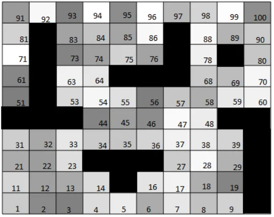
Figure 2.1: Occupancy numbered grid map.

The Figure 2.1 is the representation of the occupancy grid map. In the figure it is clear that each grid is numbered starting from 1 to 100, the black objects represent the obstacles that have occupied the grids.

2.2 Introduction to Ant Colony Optimization

(25)

multiple ants can cooperate to form an enormous social group to accomplish many other complicated tasks. The ants initially wander randomly to explore the envi-ronment near their nest, while searching for food. Different paths can be chosen by different ants to explore in compliance with their random behavior [6]. As soon as a food source is determined by an ant; it carries a bearable amount of food on its way back to its nest.

By a lot of research and study; biologists have found that ants leave some chemical substance on the paths that were traversed by them, which is called pheromone, and the quantity of pheromone is inversely proportional to the length of the route. It was also mentioned in Dorigo’s research in 1992 that the ants can also perceive the pheromone when they pass the path, and their actions could be influenced by the concentration of pheromone. However, the amount of the pheromone left may vary depending on the quality and quantity of the food. Then, other ants now can choose the route that has denser pheromone (which can be treated as a better route) and guides them to the food source. This behavior will also cause the formerly better path to becoming even much better by aggregating more pheromones. This behavior of the ants is depicted in Figure 2.2.

(26)

We can see that the nest of the ants in Figure 2.2 is denoted by A and the food source is denoted byE. In Figure 2.2 (a), (b) and (c), the space between the starting (A) and the goal positions(E) is the environment that is to be explored by the ants. In Figure 2.2(a) the ants move freely between the points A and E.

However, in Figure 2.2 (b) an obstacle is placed unevenly to cut off the path between the points A and E. The longer part of the obstacle is denoted by H, and the shorter part is denoted by C. Once the obstacle is added the ants have to now choose between the paths AC or AH to reach the food source E. At first, the ants randomly choose either of the paths AH or AC. After a considerable amount of time, the ants realize that taking the path AC makes them reach the point E faster because that is the shortest path. Therefore, more number of ants follow this path and as they leave some amount of pheromone while traversing, the concentration of the pheromone on the path AC is higher compared to that on the path AH. This eventually leads to all the ants taking the path ACE than the path AHE making the concentration of pheromone on the former path denser.

This behavior of the ant colony is termed as metaheuristic, which is said to be the main concept of the ant colony optimization which falls under the category of the approximate algorithms. The approximate algorithms are used to obtain the near-optimal solutions to solve hard combinatorial optimization problems (CO).

2.2.1 The ACO Metaheuristic

ACO has been formalized into a metaheuristic for combinatorial optimization prob-lems by Dorigo et.al in the year 1992 and 1996. A metaheuristic is a general-purpose algorithmic framework that can be applied to different optimization problems with a few modifications. For example, In order to apply ACO to a given a combinatorial optimization problem we would need an adequate model [27],

(27)

• A search spaceS defined over a finite set of discrete decision variablesXi, where

i = 1, 2, ....n.

• A set of Ω constraints among the variables.

• An objective function f:S →R+₀ to be minimized.

Figure 2.3: Example of possible construction graphs for a four-city TSP where com-ponents are associated with (a) the edges or with (b) the vertices of the graph [27].

Figure 2.3 shows the example of possible construction graphs for a four city TSP problem, as depicted by the researchers in [27]. In the Figure 2.3 (a), the components of the TSP are associated with edges that means 1,2,3,4 are the vertices(i.e, cities) and c12, c24, c34, c13, c23, c14 are the edges that show the relationship between the

ver-tices. In the Figure 2.3 (b), the components are associated with the vertices of the graph; which means that the edges are considered as nodes represented byc12, ..., c14

(28)

pheromone value τij is associated with the solution componentcij; where i and j are

the cities.

One of the essential components of the ACO metaheuristic is the pheromone model. In ACO, by traversing the fully connected graph GC(V, E); where V is the

set of vertices and E is a set of edges. The mentioned connected graph GC can be

obtained by representing the solution components C either by vertices or by edges. A partial solution is built when the ants move from one vertex to vertex along the edges of the graph. A certain amount of pheromone is deposited by the ants on the components traversed(either on the vertices or the edges). However, the amount of

4τ is dependent of the quality of the solution found. Therefore, the successive ants use the pheromone information to plan their path on the most favourable regions of search space i.e the graph. Usually, a set of n variables represent a solution; where a city is associated with each variable. For example, Xi is a variable which indicates

the city to be visited after i. The pairs of cities to be visited one after the another are represented by the solution components cij = (i, j) where, i and j are the cities;

which means that the city j should be immediately visited after city i . Therefore, in this scenario of the construction graph the vertices are the cities to be traversed and the edges are the solution components. Therefore, the ants would deposit the pheromone on the edges. However, a construction graph could also be obtained by representing solution components as vertices on which the pheromone is deposited. This method of obtaining a construction graph is not very popular but is nonetheless correct [16].

(29)

Figure 2.4: ACO Algorithm [2].

The three main algorithmic components: ConstructAntSolutions, ApplyLocalSearch, UpdatePheromones are explained further in detail.

• ConstructAntSolutions

Artificial ants can be viewed as probabilistic useful methods that collect ar-rangements as progressions of parts of the arrangement. The limited arrange-ment of finite set of the solution components C = cij where i = 1, ..., n and

j = 1, .... |Di | [2]. A solution construction commences from an empty partial

solutionSp =∅. At every construction step, the partial solutionSp is elongated

by adding a feasible solution component from the set N(Sp) ⊆ C, which is

defined as the set of components that can be appended to the current partial solution Sp without violating any of the constraint values. The determination

of a solution component from N(Sp) is supervised by a stochastic mechanism,

which is biased by the pheromone correlated with each of the elements ofN(Sp). • ApplyLocalSearch

LocalSearch is usually included in state-of-the-art ACO algorithms [6]. Af-ter all the ants finished the partial solution construction in one iAf-teration, the pheromone should be updated to increase its value to keep a strong association with the good or promising solutions. There are two main steps:

(30)

– Increase the pheromone levels associated with a chosen set of good solu-tions.

Once solutions have been built, and before refreshing the pheromone, it is com-mon to augment the solutions obtained by the ants by a local search. This phase, which is exceptionally problem-specific, is optional although it is usually included in state-of-the-art ACO algorithms.

• UpdatePheromones

The pheromone update aims to raise the pheromone values correlated with ben-eficial or promising solutions and to reduce those that are associated with poor ones. Usually, this is obtained (i) by lowering all the pheromone values through pheromone evaporation, and (ii) by raising the pheromone levels associated with a chosen set of good solutions.

2.2.2 Main ACO Algorithms

A lot of research on the ACO algorithms and their implementation has been done previously; such as in [23], [6], [11], [21] and [24] among the others. The main ACO algorithms are:

• Ant System Algorithm (AS)

• Ant Colony System Algorithm (ACS)

• Max-Min Ant System Algorithm (MMAS)

(31)

Ant System Algorithm

Ant System is the first ACO algorithm proposed in the literature [7] and [9]. The main characteristic of this algorithm is that the pheromone values are updated by all the m ants that have built a solution, at each iteration.

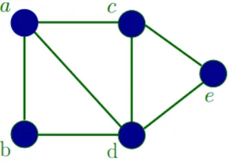
Figure 2.5: Construction Graph.

For example, assume the Ant System as a connected construction graph consisting of vertices and edges as shown by Figure 2.5; represents a 5 city TSP problem. In the figure 2.5 the nodes a,b,c,d,e are the cities and the lines connecting them are the edges. Here, for a vertex pair (ab) and edge (a,b), the pheromone would be denoted byτab, associated with the edge joining cities a and b, is updated as follows:

τab ←(1−ρ).τab+ Σmk=14τ k

ab (2.1)

where ρ is the evaporation rate, m is the number of ants, and the quantity of pheromone deposited on edge (a, b) by ant k which is denoted by 4τ_abk. It can be represented by the equation (2.2) where Q is a constant, and Lk is the length of the

tour constructed by ant k in the present iteration.

τ_abk =

     Q Lk

, if ant k used edge (a,b) in its tour 0, otherwise

(32)

By having the τab value, the probability for ant k to go to vertex b from a is

calculated as shown in the equation (2.3).

P_abk =

       τα ab.η β ab

ΣCal∈N(sp).τ

α al.η

β al

if Cab ∈N(sP),

0 otherwise,

(2.3) In equation (2.3) the first condition is satisfied only if Cab belongs to the set of

possible components which is here denoted by N(Sp). It means that vertices (a,l)

where l is a city not yet visited by the ant k. The relative effect of the pheromone versus the heuristic information ηab is controlled by the parameters α and β, which

is given by the equation (2.4), wheredab is the distance between cities a and b,

ηab =

1

dab

(2.4) Similar to which the process was described in theoretical explanation in Section 2.2.1, in each iteration, based on the paths traveled by each ant, the pheromone τab

on each edge of the connected construction graph is updated using equation (2.2). Ants will traverse through the graph probabilistically choosing next vertex by us-ing equation (2.3) when the next round of iteration begins, based on the updated pheromone.

Ant Colony System

(33)

According to [13], the three main aspects in which the ACS differs from the Ant System are:

i) A direct way to balance between the exploration of new edges and exploitation of a priori and registered knowledge on the problem is provided by the state transition rule.

ii) The global updating rule is applied only to edges which relate to the best ant tour.

iii) A local pheromone updating rule (local updating rule, for short) is applied while ants are constructing a solution. The quantity of pheromone on the traversed edges is updated by the ants while constructing their tour using the local updating rule. The pheromone updating rules are outlined so that they tend to give more pheromone to edges which should be visited by ants [13].

2.3 MAX-MIN Ant System

The Max-Min algorithm was first proposed in the year 2000 by T. Stutzle and H.H. Hoos. Many studies were conducted on ACO [4], [23], [26] which have shown that by stronger exploitation of the best solutions (obtained during the search and the exploration of the environment) the performance of the algorithm could be improved. However, in [24] the author has introduced the concept of using a greedier search in the MMAS algorithm; the introduced concept potentially aggravates the problem of premature stagnation of the search. MAX-MIN Ant System differs in three key aspects from the Ant System, namely:

(34)

of the trial (global-best ant).

• The range of possible pheromone trails on each solution component is limited to an interval [τmin, τmax], to avoid stagnation of the search [24].

• The pheromone trails are initialized to τmax, to achieve a higher exploration of

solutions at the beginning of the algorithm [24].

Pheromone Trial Updating

The modified pheromone trail update rule is given by

τij(t+ 1) =ρτij(t) +4τijbest (2.5)

where [∆τ]best

ij = 1/(Lbest); here, Lbest is the length of the tour of the best ant.

It could either be the best tour found in the present iterationiteration-best, Lib or

the best solution found since the initialization of the algorithm Lbs (best so far) or a

combination of both.

The notion of convergence for MAX-MIN Ant System which is needed in deter-mining the values of pheromone trial limits was introduced in [24]. The concept of convergence of MMAS differs in one slight but important aspect from the concept of stagnation [10]. All ants follow the same path in stagnation. However, in situations of convergence, it is not the similar case due to the use of the pheromone trail limits.

Pheromone trail initialization

In MMAS the pheromone trails are initialized in such a way that after the first iter-ation all pheromone trails correspond to τmax(1). The strategy of all the pheromone

trials corresponding to τmax(1) can easily be achieved by setting τ(0) to some

(35)

first iterations of the algorithm, this type of trail initialization is chosen to increase the exploration of solutions.

2.4 Changes made to the MMAS Algorithm

2.4.1 Addition of Diversification mechanisms[24]

The diversification mechanism is used and to check if that allows MMAS to converge to a very high-quality solution. Two variants which contrast in the degree of search diversification are examined. Firstly, the pheromone trials are reinitialized toτmax as

given below,

τ_ij∗(t) =τij(t) +δ(τmax(t)−τij(t)) (2.6)

However, this corresponds to setting δ = 1 in the equation above whenever the pheromone trail strengths on almost all paths are not contained in Sgb(global best

solution) are very close to τmin (minimun pheromone value).

Once the algorithm is reinitialized, the search fgb (iteration best solution) is

ap-plied as done at the start of the algorithm. The best solution found since the reini-tialization of the pheromone trials is used instead of Sgb, by doing this more search

diversification is obtained. The Max-Min Ant System algorithm is then allowed to converge to another high-quality solution.

2.4.2 Addition of local search routines[24]

(36)

neighborhood for an correcting solution. If such a solution is found, it displaces the current solution, and the local search resumes. These steps recur until no improving neighbor solution can be attained in the neighborhood of the current solution and the algorithm ceases in a local optimum (the best solution in among the available solutions in a neighborhood in an environment).

2.5 Literature Review and Related Work

In [10] the authors proposed the ant system as a new approach to stochastic com-binatorial optimization. They have studied the performance of the ACO algorithm on a TSP problem in a static envirnment. Their basic idea was that if at a given point an agent (ant) has to choose between different options for its next move and the one actually chosen results to be good, then in the future that choice will appear more desirable than it was before. Also, the authors in [10] have shown that the Ant System problem could be applied to different CO problems.

The authors in [10] introduced the ACO meta heuristic algorithm. The ACO meta heuristic was implemented on a TSP problem in a static environment. They have also discussed the importance of the trial visibility and Trial persistence.

Later, in [24] the authors have introduced the MMAS algorithm. The algorithm’s performance was evaluated when implemented o a TSP problem. The results obtained indicated that the performance of the algorithm was better when compared to the ACO algorithm as the former one uses a greedier search.

(37)

(38)

Chapter 3 Environment Modeling and the

Working of MMAS

3.1 Modeling of Robot Motion Environment

Autonomous navigation describes a higher level of performance since it applies ob-stacle avoidance simultaneously with the robot steering toward a given target [4]. Therefore, it implies an environment with known and unknown obstacles, and it in-corporates global path planning algorithms [3] to organize the robots path amidst the known obstacles, as well as local path planning for real-time obstacle escape.

(39)

we used in our experiments are the occupancy grid maps.

An initial implementation of occupancy grid maps was used by Moravec in his research in 1988 to automatically prepare a map of the environment. Sensor readings were matched to the map, altering the possibility that observed cells are filled. For example, a sonar sensor returns the nearest object within a cone, so the cells in the extent of the cone closer than the reading are probably unoccupied. Moravec in 1988 represented each cell in his reasearch as a possibility of being traversable and initializes them to an obscure value. He illustrated a probabilistic technique to update cells for several types of sensors and supplied a procedure to permit the map to be renewed as the robot moves [15].

According to Milstein’s research in 2008 in [18], to build an occupancy grid map, it is required to determine the occupancy probability of each cell. Although, assumed that it is not surely accurate, especially when acknowledging nearby cells representing the equivalent physical object. As a result, the probability of a distinct map m, can be factored into the product of the different probabilities of it’s cells.

The probability of a precise cell is simple to ascertain, given the robots location and sensor readings since it is defined by whether the robot observes the cell as unoccupied or occupied [18]. The Occupancy grid mapping refreshes a map according to a sensor reading at a location so that, as evidence accrues, the map becomes accurate.

Milstein in his research in [18], mentioned an example where we consider each cell of the map to be an independent object, which can be either present or absent. Although independence is usually not entirely valid, it was assumed to be so.

The assumptions can therefore be summarized as follows:

(1) 2D definite space is the environment in which the mobile robot moves.

(2) The movable trajectories of the dynamic objects can be estimated for the future, keeping the speed of the robot constant.

(40)

environment information can be centered in the current grid center [18].

3.1.1 Robot movement in grid environment

In a grid environment, the number of obstacles are lesser in number in some instances compared to the others depending on the experiments being constructed (it is a decision to be made by the researcher.

Figure 3.1: An example of the grid map.

(41)

The robot aims to search an optimal or near optimal path from the start to the destination grid (goal). We adopt two main methods for grid marking, namely the Rectangular coordinate method and the Serial number method.

• Serial number method: From the bottom left of the grid map, coding the grid from bottom to top, from left to right as shown in Figure 3.1. The serial number is from 1 to 100. The grid using the serial number method to mark is

gn, e.g., the grid of serial number 1 is marked as g1.

• Rectangular coordinate method: The method in which every grid coordi-nate is indicated with central point (x, y). The grid using Rectangular coordi-nate method isg(x, y), e.g., the grid of serial number 1 is marked as g(0.5,0.5). The starting point of robot path planning is assigned as g1 in the bottom left

of the map, likewise, the target point of robot path planning as g100.

To simulate the real ant colony seeking food behavior in the given example in the Figure 3.1, we assume that the starting point of robot path planningg1, and the

target point gn as a food source.

3.2 Theoretical Explanation of Path Planning

Once the modeling of the environment and the process of marking the grid is done, we would initialize the robot at grid g1 and wait for it to navigate itself through

the environment and reach the grid g100.As discussed in Section 1 Navigation is a

methodology that allows guiding a mobile robot to achieve a mission through an environment with obstacles healthily and safely. The two basic tasks included in navigation are the localization, and path planning.

(42)

In the experiments implemented in this thesis, we have used grid maps with obsta-cles. The ants have a planned path from the starting to the goal position. However, once the algorithm is implemented, and a new obstacle is added everytime, in a while the agents would have to re-route their path from their current position which is assumed to be the start position after a new obstacle is added, and then a path is planned from that point to the goal position.

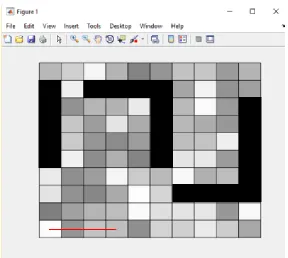
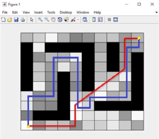
This process is repeated every time a new obstacle is added. The Figures 3.2, 3.3, 3.4 depict the way the robots plan their path. In these figures the black and the grey objects represent the obstacles, the red line represents the path travelled by the ants , the dotted red line represents the previous path travelled by the ants; the grid on the bottom most left is the starting position of the ants and the grid on the top most right is the goal position. The process of path planning and path rerouting is further explained in detail.

(43)

Figure 3.2: The example of path re-routing(a).

(44)

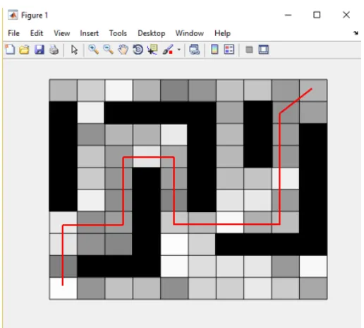
Figure 3.3: The example of path re-routing(b).

The ants finally reach the destination grid after rerouting their path every time they encounter an obstacle. This is shown in the Figure 3.4.

(45)

3.3 Robot Path Planning Based on Max-Min

Al-gorithm

In the research of the MMAS algorithm, it has been found that the algorithm solves the TSP problem successfully. But before applying MMAS on the field of robot path planning, many changes to the traditional algorithm have to be made based on the features of robot path planning. It introduces τmax (upper) and τmin (lower) bounds

to the values of the pheromone trails, as well as a distinctive initialization of their values.

In practice, the permitted range of the pheromone trail strength is limited to the interval that is [τmin, τmax], and the pheromone trails are initialized to the upper trail

limit, which induces a higher exploration at the start of the algorithm [24]. The MMAS algorithm was modified by Stuzle et.al in the year 2000 after he introduced the algorithm in the year 1999, to achieve faster convergence speeds while still finding shorter paths.

(46)

Chapter 4 Analysis, Evaluation of Results and

Discussion

In this chapter, we shall discuss the experiments conducted in detail. Also we have summarized and analyzed all of the results obtained.

4.1 Simulation

All the experiments were conducted on a PC with device specifications a 3.40GHz Intel CORE i7-6700 processor, 8 GB of RAM and 64-bit Windows operating system.

All the simulation programs have been compiled using MATLAB.

4.2 Parameter Settings

• The number of ants m:

(47)

the convergence speed is slowed down, on the contrary, if the number of ants m

is too few, the stability of the algorithm is reduced, and the problem of early stagnation would occur [12]. In our thesis we have set the number of ants as 20 for the grids 10x10, 20x20 and 40x40. However, the number of ants required to implement the algorithms for the grids 100x100, 200x200 and 400x400 had to be more than 20 since the grid maps are of large sizes an it would help in better exploration of the environment and converge to a near optimal solution in feasible amount of time. However, when we initially used just 20 ants for the larger grid environments, we came across few problems which will discussed in the Section 4.5.

• The combination of parameters α, β, ρ:

The relative importance of pheromone accumulated by ant colony is reflected by

α which is the impact index of pheromones, and the relative importance of the heuristic information is reflected by β which is the impact index of a heuristic factor.

The pheromone evaporation rate ρ reflects the intensity of the interaction be-tween ants, which is directly related to the global search ability and conver-gence speed of the ACO and related algorithms. The global search ability of the MMAS algorithm can be improved by increasing the value of ρ. However, the convergence speed of the algorithm is reduced.

(48)

• The pheromone values τmax and τmin:

In MMAS, we set the maximum pheromone trail τmax to an estimate of the

asymptotically maximum value.

To determine reasonable values for τmin , we use the following assumptions as

mentioned in [24],

– The best solutions are found shortly before search stagnation occurs. In such a situation the probability of re-constructing the global-best solution in one algorithm iteration is significantly higher than zero. Better solutions may be found close to the best solution found.

– The main influence on the solution construction is determined by the rel-ative difference between upper and lower pheromone trail limits, rather than by the relative differences of the heuristic information.

Stutzle and Hoos have introduced a formula to calculate the maximum and the minimum trial limit values which are assumed to be approximate [24].

τmin =τ max.

1−(Pbest) −(1−n)

avg−1(Pbest)−(1−n)

(4.1) where avg is the average number of components that can be chosen in con-struction steps, Pbest is the probability of constructing the best solutions, and

n represents the number of components in the constructed solution.

• Pheromone Intensity Q:

(49)

the algorithm easily fall into a local optima.

• The number of iteration Nc:

To ensure the algorithm can search the optimal path within the number of iterations, the value of Nc should be set larger. In this thesis, under the 10*10

grid environment map, Nc = 100, under the 20*20 grid environment map, Nc

= 400, under the 40*40 grid environment map, Nc = 1600, under the 100*100

grid environment map, Nc = 10000, under the 200*200 grid environment map,

Nc = 40000, under the 400*400 grid environment map,Nc = 160000.

4.3 The Implementation of Simulation Experiments

The aim of the thesis as mentioned in Section 1.3 is to implement the improved MMAS algorithm in larger dynamic grid maps. However, we have not only implemented the MMAS algorithm in a smaller grid environment but also on a larger environment to check for its scalability. Obstacles are set in every map whose position is unknown to the robot The experiments are later performed on 6-different sizes of the grid maps. The performance of the MMAS is also studied and compared with the ACO algorithm on different maps implemented by the previous researchers.

4.3.1 Collection of Maps Used in the Experiments

(50)

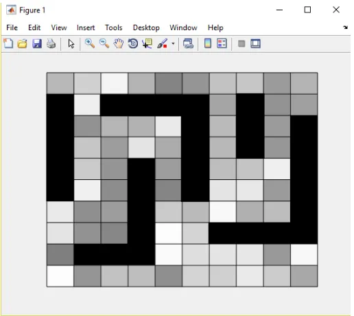
Figure 4.1: Map1: 10*10 Grid environment.

(51)

(52)

(53)

(54)

(55)

Figure 4.12: Map2: 400*400 Grid environment. The Figures 4.11 and 4.12 represent the 400*400 grid maps.

(56)

the algorithm on a map M; where M represents all the scenarios of the maps in which the algorithm was implemented which are denoted as map1, map2, map3 etc. During the first iteration the obstacles are placed in the grid g3, g6, g7 which we can

consider as map1; once a best path is found the positions of the obstacles are changed fromg3, g6, g7 to g5, g8, g9 which is considered as the map2 on which the algorithm is

implemented again with a record of the pheromone values that were updated after finding the best path in map1. Again in map3 the positions of the obstacles are changed and the implemented again without re-initializing it. Similarly, the positions of the obstacles is changed for every iteration and the algorithm is implemented until it reaches the maximum number of iterations. Sometimes, once the position of the obstacles is changed and the obstacle might not be in the grids that are a part of the best path, therefore it would not cause any changes to the path length. As we use the pheromone update rules, by the time the algorithm reaches the maximum iteration the best paths found at every iteration would contain a pheromone value. But there would be one path with the most concentration of pheromone, it is known as the near-optimal path. The length of the near-optimal path is the value of the convergence rate of the algorithm. Therefore, we note the iteration at which the algorithm has begun to converge and gives the same path length(which is the optimal path length) until the maximum iteration is reached. In our approach since we utilize all the iterations as well as all the pheromone values in order to narrow down to the optimal path value; we can say that we do not waste any of the resources or the parameters used.

4.3.2 Collection of the Results

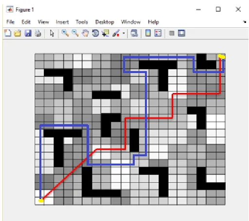
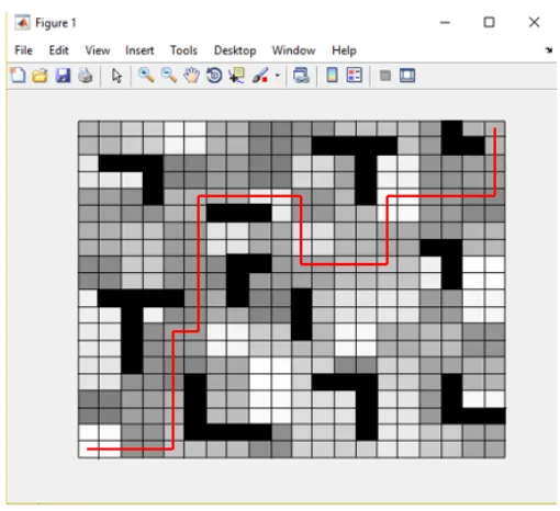
In this subsection we represent the grid maps with the paths obtained after the algorithms were implemented.

(57)

4.19, 4.20 represent the 20*20 grid maps; The Figures 4.21, 4.22, 4.23, 4.24 represent the 40*40 grid maps; The Figures 4.25, 4.26, 4.27, 4.28 represent the 100*100 grid maps; The Figures 4.29, 4.30, 4.31, 4.32 represent the 200*200 grid maps; The Figures 4.33, 4.34, 4.35, 4.36 represent the 400*400 grid maps. In a 10*10 grid map, the grids are numbered from 1 to 100, with the grid1 being the starting point and the grid100

being the destination point. The start and the destination grids are marked with yellow dots in the maps. The blue line represents the predicted path (for the MMAS algorithm) and the red line represents the near optimal path found by the algorithms. The values obtained (the length of the paths and the other parameters) by imple-menting these algorithms are shown and discussed in the next section.

(58)

Figure 4.14: Map2: 10*10 Grid environment after the (near) optimal path is found by MMAS.

(59)

(60)

Figure 4.18: Map2: 20*20 Grid environment after the (near) optimal path is found MMAS.

(61)

Figure 4.20: Map2: 20*20 Grid environment after the (near) optimal path is found ACO.

(62)

(63)

Figure 4.24: Map2: 40*40 Grid environment after the (near) optimal path is found ACO.

(64)

(65)

Figure 4.28: Map2: 100*100 Grid environment after the (near) optimal path is found by ACO.

(66)

(67)

(68)

(69)

4.3.3 Summary of the values obtained upon implementation

of the algorithms

(70)

Maps MMAS Iteration for MMAS ACO Iteration for ACO

Path Length Time(seconds) Optimal Conv Path Length Time(seconds) Optimal Conv

Experiment 1

Map1 15.6476 10.35 6 54 24.6476 14.72 9 59

Map2 17.8955 13.05 8 56 24.8955 16.46 12 62

Experiment 2

Map1 33.7568 16.78 25 216 47.7568 23.45 33 236

Map2 36.8429 18.56 31 224 47.8439 25.24 44 248

Experiment 3

Map1 84.7652 149.45 96 864 97.5624 153.61 130 944

Map2 88.6476 168.89 128 896 102.6332 174.43 176 992

Experiment 4

Map1 212.5926 165.79 623 5402 218.6476 174.64 927 5920

Map2 224.2841 182.96 801 5780 231.4457 210.56 1253 6271

Experiment 5

Map1 492.53 208.91 2405 21601 510.75 217.72 3618 23690

Map2 523.86 227.59 3244 22495 547.56 241.95 4877 24802

Experiment 6

Map1 1074.56 546.24 9601 86404 1102.62 589.68 14421 94400

Map2 1124.47 696.79 12804 89609 1149.85 748.46 19220 99204

Table 4.1: Summary of the values obtained after the implementation of MMAS and ACO algorithms.

(71)

of 24.8955 in 16.46 seconds in the 12th iteration and the convergence rate is obtained at 62nd iteration.

Upon looking at the Table 4.1 carefully, we can notice that for the experiments performed the path length obtained by the MMAS algorithm in almost all of the scenarios is less when compared to the ACO algorithm. It is also clear that the time taken by the ACO algorithm to find a path is also more when compared to the MMAS algorithm.

However, the performance of the MMAS algorithm slows down as we increase the size of the grid maps. In the Experiment number 2 where we use a 20*20 grid map number 1 the optimal path length obtained is 33.7568 in 16.78 seconds and the path length was obtained at 25th iteration whereas the convergence was achieved at 216th iteration. For the same map the path length obtained by the ACO is 47.7568 in 23.45 seconds at 33rd iteration and converges at the 236th iteration. The values obtained by the algorithms when implemented in a 40*40 grid map that is the Experiment number 4 are 84.7652 in 149.45 seconds at 96th iteration and convergence is at 864th iteration; for the MMAS. In the same map the path length is 97.5624 in 153.61 seconds at 130th iteration and the convergence at the 944th iteration; for the ACO.

(72)

4.4 Evaluation of the Results

4.4.1 Performance Evaluation Indexes

In order to comprehensively measure the performance of the ant colony algorithm, the following basic indexes to evaluate the performance of ant colony algorithm are used which have been introduced in [28]:

The Best Performance Index:

Let EO represents the best performance index, the formula is as follows:

Eo =

cb−c∗

c∗ ∗100 (4.2)

where cb represents the optimal value obtained by the algorithm; c* represents

the theoretical optimal value. When the theoretical optimal value is unknown,it is replaced by the best known value. The optimal performance index is used to measure the optimal optimization degree of the ant colony algorithm. The smaller of the value means that the optimal performance of the ant colony algorithm is better.

The Time Performance Index

Let ET represents the time performance index, the formula is as follows:

ET =

Ia∗T0

Imax

∗100 (4.3)

where Ia represents the algorithm’s number of iterations when it meets

conver-gence condition(In this paper, Ia refers to the iteration number when the mean path length tend to be stable); T0 represents the average execution time of one iteration;

Imax represents the algorithm’s number of iterations. The time performance index is

(73)

means that the convergence speed of the ant colony algorithm is quicker.

The Robustness Performance Index

Let ER represents the robustness performance index, the formula is as follows:

ER =

ca−c∗

c∗ ∗100 (4.4)

where ca represents the average path length value; c* represents the theoretical

optimal value. When the theoretical optimal value is unknown, it is replaced by the best known value. The smaller of the ER means that the stability of the ant colony

algorithm is better.

4.4.2 Performance Evaluation of the Algorithms

(74)

MAP1 MAP2

Eo ET ER Eo ET ER

Experiment 1

MMAS 0.18 2.26 0.6 0.25 2.34 1.1 ACO 0.27 3.62 1.0 1.8 4.88 2.7 Experiment 2

MMAS 0.85 2.92 8.6 1.3 3.98 4.83 ACO 3 4.11 9.1 4.16 6.78 11.2 Experiment 4

MMAS 2 9 18.52 3.8 7.2 21.2 ACO 5.3 13.2 22.31 9.74 11.35 29.37 Table 4.2: Performance Evaluation of the results.

Looking at the performance evaluation results shown above in the Table 4.2, we can incur that the Best performance index of the MMAS algorithm is always less than that of the ACO algorithm. For example, in Experiment 1; for the MMAS and the ACO the E0 = 0.18percentand E0 = 0.27percent. It means that the performance of

the MMAS algorithm was better in the MAP 1 when compared to the performance of the ACO algorithm. The time performance index and the robustnes performance index are also evaluated for. A similiar kind of performance trend as in MAP 1 was observed when the algorithms’ performances were evaluated in MAP 2.

(75)

As mentioned in the Subsection 4.4, the smaller the values of E0, ET, ER; the

better is the performance of the algorithm. Therefore, if we compare all the values of the MMAS performance indexes to the values of the ACO performance indexes we can say that the MMAS has performed better than the ACO algorithm in the experiments.

The Figure 4.37 and 4.38 are the graphical representation of the comparison of the performance evaluation indexes of the two algorithms in the MAP 1 and MAP 2; as shown in the Table 4.2.

Figure 4.37: Performance comparison of MMAS and ACO in MAP 1.

(76)

4.5 Discussion

In the Experiment 1 implemented on 10*10 grid maps, the MMAS and the ACO algorithms have performed well because they were able to converge to a near optimal solution in the end. However, the MMAS was able to converge to a solution faster.

In the Experiment 2 and 3 where the MMAS and the ACO Algorithms were implemented on a 20*20 and 40*40 grid maps, the MMAS algorithm was still able to find the solutions quicker than the ACO algorithm.

However in Experiment 4,5 and 6( in the 100*100, 200*200, 400*400); the MMAS has slowed down a bit when compared to its speed in the previous Experiments 1,2,3. The ACO algorithm has been performing relatively slow when compared to the MMAS overall. As the size of the search space that is the size of the maps increases the convergence speed of the algorithms has reduced drastically.

On comparing the performance of this algorithm with that of the ACO on all the six set of map sizes, we can say that the performance of the MMAS is better than that of the ACO algorithm because the ACO converges to a solution late than the improved MMAS algorithm. Larger grid maps such as 40*40, 100*100, 200*200 and 400*400 haven’t been used before by researchers to implement the algorithm and check for its scalability. Therefore experiments have been conducted in the larger grid maps which are also one of the main contributions of this thesis. The optimal path obtained by the algorithm in the environment after the change in the obstacles position is shown in the Figures 4.13, 4.14, 4.3, 4.4, 4.21, 4.22, 4.25, 4.26, 4.29, 4.30, 4.33, 4.34 . Comparing the time taken by the algorithm we can see that its capability to do so is more in the smaller environments even if the agents had to reroute their path because of the increase in the workspace area.

(77)

the best solution that has been found since the re-initialization of the pheromones is used which is in turn increasing the search diversification. That helped the MMAS algorithm to converge to a better quality solution which is the near optimal path in our experiments. Also, using the technique of adding local search routines where the algorithm is constantly searching for better solution in its neighborhood and if one such solution is found then it replaces that with the current solution. The algorithm has repeated this process until no better solution could be attained in the neighborhood.

(78)

Chapter 5 Conclusion and Future Work

This thesis mainly focuses on the mobile Robot Path Planning Problems based on the Ant Colony Optimization variant algorithm, i.e., the Max-Min Ant System Algorithm. To be specific, the research work of the thesis is listed below:

• Firstly, the actual working environment of the mobile robot is modeled. Envi-ronmental modeling adopts grid method. The actual working environment is divided into grids of the same size, and the grids are containing obstacles are grayed out. Two methods; Serial number method and the rectangular coordi-nate to identify all grids and they could be well commuted to each other. The other Robot Path Planning problem based on the Ant Colony Algorithm is a process that through the interaction and cooperation between the individual of the ant colony, they will avoid all obstacles to find an optimal path from the starting grid to the target grid.

• Secondly, we made modifications to the MMAS algorithms as per the techniques introduced by previous researchers . For example, we applied diversification mechanisms based on the pheromone initialization and addition of local search routines that are described in Section 2.4

(79)

maps of 6 different sizes to verify the validity and effectiveness of the MMAS Algorithm under the different maps used.

Several conclusions could be summarized through the results of the six group experiments:

• The ability of the MMAS algorithm to find the optimal solution, convergence speed and stability are higher when implemented on a grid map of smaller size.

• When dealing with the grid maps of larger sizes the ability of the algorithm to search the near optimal solution is same but the time taken is on an increasing trend with the increase in the size of the map.

• However, the speed and stability are fast in a smaller environment when com-pared to the large maps, no matter how the complexity of the map and the start and the destination path vary.

We could conclude by saying that MMAS is suitable and effective in solving RPP considering its processing time and stability. However, the research work in this thesis also has some limitations mainly reflecting on the following aspects.

• The experiments in this thesis are set on a grid map, instead performing on the real-time environment could be done in the future work.

(80)

Bibliography

[1] Jens Christian Andersen. Mobile robot navigation. 2007.

[2] Christian Blum. Ant colony optimization: Introduction and recent trends.

Physics of Life reviews, 2(4):353–373, 2005.

[3] Johann Borenstein and Yoram Koren. Optimal path algorithms for autonomous vehicles. InProceedings of the 18th CIRP Manufacturing Systems Seminar, pages 5–6, 1986.

[4] Michael Brand, Michael Masuda, Nicole Wehner, and Xiao-Hua Yu. Ant colony optimization algorithm for robot path planning. InComputer Design and Appli-cations (ICCDA), 2010 International Conference on, volume 3, pages V3–436. IEEE, 2010.

[5] N Buniyamin, N Sariff, WAJ Wan Ngah, and Z Mohamad. Robot global path planning overview and a variation of ant colony system algorithm. International journal of mathematics and computers in simulation, 5(1):9–16, 2011.

[6] Marco Dorigo. Optimization, learning and natural algorithms. PhD Thesis, Politecnico di Milano, 1992.

(81)

In-ternational Conference, ANTS 2008, Brussels, Belgium, September 22-24, 2008, Proceedings, volume 5217. Springer, 2008.

[8] Marco Dorigo and Luca Maria Gambardella. Ant colony system: a cooperative learning approach to the traveling salesman problem. IEEE Transactions on evolutionary computation, 1(1):53–66, 1997.

[9] Marco Dorigo, V Maniezzo, and A Colorni. Positive feedback as a search strategy. dipartimento di elettronica, politecnico di milano. Technical report, Italy, Tech. Rep. 91-016, 1991.

[10] Marco Dorigo, Vittorio Maniezzo, and Alberto Colorni. Ant system: optimiza-tion by a colony of cooperating agents. IEEE Transactions on Systems, Man, and Cybernetics, Part B (Cybernetics), 26(1):29–41, 1996.

[11] Marco Dorigo and Thomas St¨utzle. The ant colony optimization metaheuristic: Algorithms, applications, and advances. In Handbook of metaheuristics, pages 250–285. Springer, 2003.

[12] Hai-Bin Duan. Ant colony algorithms: theory and applications. Chinese Science, 2005.

[13] Luca Maria Gambardella and Marco Dorigo. Solving symmetric and asymmetric tsps by ant colonies. In Evolutionary Computation, 1996., Proceedings of IEEE International Conference on, pages 622–627. IEEE, 1996.

[14] Gengqian Liu, Tiejun Li, Yuqing Peng, and Xiangdan Hou. The ant algorithm for solving robot path planning problem. In null, pages 25–27. IEEE, 2005. [15] Mauro Birattari Marco Dorigo and Thomas Stutzle. Sensor fusion in certainty

(82)

[16] Mauro Birattari Marco Dorigo and Thomas Stutzle. Ant colony optimization artificial ants as a computational intelligence technique. IEEE COMPUTA-TIONAL INTELLIGENCE MAGAZINE, pages 28–39, 2006.

[17] Hui Miao and Yu-Chu Tian. Robot path planning in dynamic environments using a simulated annealing based approach. 2008.

[18] Adam Milstein. Occupancy grid maps for localization and mapping. In Motion Planning. InTech, 2008.

[19] G Nirmala, S Geetha, and S Selvakumar. Mobile robot localization and naviga-tion in artificial intelligence: Survey. Computational Methods in Social Sciences, 4(2):12, 2016.

[20] Purushothaman Raja and Sivagurunathan Pugazhenthi. Optimal path plan-ning of mobile robots: A review. International Journal of Physical Sciences, 7(9):1314–1320, 2012.

[21] Valéria de C Santos, Fernando S Osório, Cláudio FM Toledo, Fernando EB Otero, and Colin G Johnson. Exploratory path planning using the max-min ant system algorithm. InEvolutionary Computation (CEC), 2016 IEEE Congress on, pages 4229–4235. IEEE, 2016.

[22] Alexander Schrijver. A course in combinatorial optimization. TU Delft, 2000. [23] Thomas St¨utzle and Marco Dorigo. Aco algorithms for the traveling salesman

problem. Evolutionary algorithms in engineering and computer science, pages 163–183, 1999.

(83)

[25] Ioan Susnea, Viorel Minzu, and Grigore Vasiliu. Simple, real-time obstacle avoidance algorithm for mobile robots. In 8th WSEAS International Conference on Computational Intelligence, Man-Machine Systems and Cybernetics (CIM-MACS09), 2009.

[26] Guan-Zheng Tan, Huan He, and Aaron Sloman. Ant colony system algorithm for real-time globally optimal path planning of mobile robots. Acta automatica sinica, 33(3):279–285, 2007.

[27] Sebastian Thrun, Wolfram Burgard, and Dieter Fox. Probabilistic robotics. MIT press, 2005.

(84)

Appendix-Abbreviations

• ACO : Ant Colony Optimization

• ACS : Ant Colony System

• AS : Ant System

• MMAS: Max-Min Ant System

• CO : Combinatorial Optimization

(85)

Vita Auctoris

NAME: Satya Shree Sankini PLACE OF BIRTH: Telangana,India

Performance evaluation of Max-Min Ant System Algorithm for Robot Path Planning in Grid Environment