Detecting understory plant invasion in urban forests using LiDAR

(1)

International Journal of Applied Earth Observation and Geoinformation 38 (2015) 267–279

Contents lists available atScienceDirect

International Journal of Applied Earth Observation and

Geoinformation

j o u r n a l h o m e p a g e :w w w . e l s e v i e r . c o m / l o c a t e / j a g

Detecting understory plant invasion in urban forests using LiDAR

Kunwar K. Singh

a,∗

_{, Amy J. Davis}

b

_{, Ross K. Meentemeyer}

a

a_{Center for Geospatial Analytics, Department of Forestry and Environmental Resources, North Carolina State University, Raleigh, NC 27695, USA}

b_{Department of Geography and Earth Sciences, University of North Carolina, Charlotte, NC 28223, USA}

a r t i c l e i n f o

Article history:

Received 14 October 2014

Received in revised form 18 January 2015 Accepted 22 January 2015

Available online 12 February 2015

Keywords:

Biological invasion Chinese privet Data integration IKONOS LiDAR

Ligustrum sinense

Random forest

a b s t r a c t

Light detection and ranging (LiDAR) data are increasingly used to measure structural characteristics of urban forests but are rarely used to detect the growing problem of exotic understory plant invaders. We explored the merits of using LiDAR-derived metrics alone and through integration with spectral data to detect the spatial distribution of the exotic understory plantLigustrum sinense, a rapidly spreading invader in the urbanizing region of Charlotte, North Carolina, USA. We analyzed regional-scaleL. sinense

occurrence data collected over the course of three years with LiDAR-derived metrics of forest structure that were categorized into the following groups: overstory, understory, topography, and overall veg-etation characteristics, and IKONOS spectral features – optical. Using random forest (RF) and logistic regression (LR) classifiers, we assessed the relative contributions of LiDAR and IKONOS derived variables to the detection ofL. sinense. We compared the top performing models developed for a smaller, nested experimental extent using RF and LR classifiers, and used the best overall model to produce a predictive map of the spatial distribution ofL. sinenseacross our country-wide study extent. RF classification of LiDAR-derived topography metrics produced the highest mapping accuracy estimates, outperforming IKONOS data by 17.5% and the integration of LiDAR and IKONOS data by 5.3%. The top performing model from the RF classifier produced the highest kappa of 64.8%, improving on the parsimonious LR model kappa by 31.1% with a moderate gain of 6.2% over the county extent model. Our results demonstrate the superiority of LiDAR-derived metrics over spectral data and fusion of LiDAR and spectral data for accurately mapping the spatial distribution of the forest understory invaderL. sinense.

Introduction

Biological invasions are one of the leading contributors to changes in regional and global biodiversity (Asner and Vitousek 2005; Simberloff et al., 2013). The rapid spread of invaders across a range of ecosystems makes it challenging to accurately assess the spatial distribution and abundance in a timely and cost-effective manner at a desired spatio-temporal scale (Huang and Asner, 2009). Remote sensing has facilitated advances in mapping and monitoring biological invasions across a range of ecosystems, including deciduous forests (Resasco et al., 2007), wet-lands (Laba et al., 2008), rangelands (Glenn et al., 2005), coastal environments (Hestir et al., 2008), and tropical forests (Asner et al., 2008). These successes are primarily attributable to sensor

∗_{Corresponding author at: Department of Forestry and Environmental Resources,}

North Carolina State University, Raleigh, NC 27695, USA. Tel.: +1 704 359 7139; fax: +1 919 515 3439.

E-mail addresses:[email protected](K.K. Singh),[email protected]

(A.J. Davis),[email protected](R.K. Meentemeyer).

characteristics, recent advancements in mapping algorithms, and synergistic use of datasets from multiple instruments. While some success has been achieved with high-to-moderate resolu-tion imagery, hyperspectral imagery has demonstrated the most promising results (Huang and Asner, 2009). The growing number of invasions in forests pushes the limits of remote sensing per-formance, particularly in detecting exotic plant invasions in the understory where regeneration and recruitment are most impacted by invaders (Becker et al., 2013). Canopy cover closure, canopy gap shadowing, mortality of native plant species, and terrain variabil-ity in the understory of forest ecosystems limit accurate detection of understory invaders (Asner et al., 2008). Successful detection often depends upon open views of the species of interest (Resasco et al., 2007) and the timing of remote sensing imagery to take advantage of phenological patterns in the overstory, i.e., after leaf abscission (Becker et al., 2013; Tuanmu et al., 2010). To date, detection of understory plant invasions is largely reliant on ﬁeld surveys, but cost and data collection times limit the number of locations that can be assessed. Although spatially explicit mod-els such as species distribution modmod-els (SDMs) have been used to predict the probability of invader presence in non-sampled

http://dx.doi.org/10.1016/j.jag.2015.01.012

(2)

locations, there has been little success to date in applying these models to new regions outside the study extent. Successful man-agement of broad-scale exotic invaders in the understory of forest ecosystems requires new techniques using minimal ﬁeld data for mapping their spatial distribution and abundance.

Several studies have examined the potential of using field-measured SDMs augmented with optical remote sensing to detect understory plant invaders (Estes et al., 2010; Rushton et al., 2004). Andrew and Ustin (2009) suggest that the mapping of the dis-tribution of invasives and sites prone to invasion using remote sensing can be improved by including covariates characterizing the environmental suitability of the site for the invader, such as slope, solar radiation index, and soil moisture index. Other stud-ies have examined the efficacy of moderate-to-high resolution and multi-to-hyperspectral remote sensing data to detect under-story invaders based on variability in seasonal and environmental responses (Wilfong et al., 2009). For example, spectral differences in the seasonal phenology of understory vegetation and decidu-ous tree canopy during leaf-off conditions can be used to detect understory vegetation, but success is limited to narrow windows of senescence time (Chastain and Townsend, 2007). The spatial and vertical heterogeneities of forest vegetation limit the util-ity of spectral-based approaches for detecting the structure and composition of understory vegetation even where distinguishing physiological and phenotypic characteristics of an invader exist (Homolova et al., 2013). Studies have also attempted to improve the detection of understory vegetation by using sub-pixel multivariate algorithms, such as artificial neural networks, linear mixture mod-els, and maximum entropy (Linderman et al., 2004; Tuanmu et al., 2010; Wang et al., 2009). While some studies have shown potential for using spectral remote sensing to detect understory invasives by coupling the phenological patterns and improved algorithms, questions remain regarding the efficient use of structural remote sensing.

Light detection and ranging (LiDAR) offers the possibility of accurately detecting understory invasive shrubs on the basis of their structural characteristics as distinguished from canopy species since it provides three dimensional data on the structure and arrangement of vegetation across all forest strata (Falkowski et al., 2009; Goetz et al., 2010). LiDAR data have been widely used for quantifying structural characteristics (e.g., tree diameter, height, density, and biomass) of forest stands (Hudak et al., 2008; Jaskierniak et al., 2011), mapping snags and understory shrubs (Martinuzzi et al., 2009), characterizing successional stages of for-est stands (Falkowski et al., 2009), estimating native understory vegetation cover (Estornell et al., 2011; Wing et al., 2012), and iden-tifying tree species. To complement LiDAR’s narrow spectral range, structural covariates of LiDAR have been combined with multi-to-hyperspectral remote sensing imagery to map forest structural attributes, plant species distribution, forest biomass, and forest canopy fuels (Mutlu et al., 2008; Popescu et al., 2004). To date, LiDAR technologies ‘alone’ or through ‘fusion’ with spectral data have not been leveraged to improve our ability to detect under-story plant invaders in urban forest ecosystems at regional scales. In addition, detection information is typically limited to direct LiDAR measurement (e.g., shrub height) of the plant individuals them-selves while ignoring other forest and landscape characteristics (e.g., topographic position) that may affect the distribution and growth of invaders.

In this study, we examine the utility of multi-return LiDAR data, IKONOS imagery, and the combination of data from both sensors for detecting and mapping understory invaders. Using Ligustrum sinense(commonly known as Chinese privet) as a case study, we focus on the urban to rural forests located in Mecklen-burg County, North Carolina to analyze the performance of LiDAR data, IKONOS, and the data combination. We incorporate additional

forest and landscape characteristics to detect this plant invader by analyzing combinations of datasets developed from categorized LiDAR-derived variables (overstory, understory, topography, and overall vegetation characteristics) and IKONOS spectral features (optical) using random forest (RF) and logistic regression (LR) clas-siﬁers. We then compare the top performing models and apply the best model to map the probability ofL. sinenseoccurrence across the heterogeneous study region.

Methods

Study system

The naturalizedL. sinensehas invaded over one million hectares of forests across a large portion of the southeastern United States, and the species is listed among the top invasives in many states (Miller et al., 2008). It grows in a wide variety of habitats and environmental conditions, including abandoned farmlands and dis-turbed areas, where it forms impenetrable thickets with a typical height range of 1–5 m, occasionally reaching heights of 10 m (Fig. 1). It is a prolific seed producer with a high germination rate. Its ability to tolerate both flooding and shade makes it well suited to the flood-plains and riparian zones of forests (Brown and Pezeshki, 2000). The abundance ofL. sinensethreatens forest ecosystems by alter-ing the diversity, composition, and structure of forests (Greene and Blossey, 2012). The growing threat of large-scale ecosystem modi-fication byL. sinenseis of extreme concern for land managers and conservationists in the United States (Hanula et al., 2009).

A growing number of studies have examinedL. sinenseinvasion and impacts on ecosystem services across much of the southeastern United States. The invasive has threatened to displace endangered Miccosukee gooseberry (Ribes echinellum) in Florida (Langeland and Burks, 1998). Invasions byL. sinensehave been linked to several negative outcomes including reduced herbaceous species in under-story and suppressed tree regeneration in a mixed hardwood forest in western North Carolina (Merriam and Feil, 2002); decreased beetle diversity in northeastern forests of Georgia (Ulyshen et al., 2010); and declining populations of the Schweintz’s sunﬂower (Helianthus schweinitzii) found in the central Piedmont region of North and South Carolina (USFWS, 1991).Faulkner et al. (1989) found that dense thickets ofL. sinensein forested areas of Tennessee produce large quantities of litter and act like ‘umbrellas’ preventing the inﬁltration of leaf litter from the native tree canopy.L. sinense ranked fourth among the top invasive plants in North Carolina with high prevalence in urban areas (EDDMapS, 2014).

The highly fragmented and urbanizing forested landscape of Mecklenburg County (1415 km2_{), located in the CMR of North}

Car-olina within the Piedmont province of the southeastern United States (Fig. 2a), provides an ideal system for this case study. The study system is characterized by rolling topography with a forest–farmland mosaic that comprises a mix of secondary growth oak–hickory–pine forests and stands of loblolly pine, which domi-nate clear-cuts and abandoned farmlandSingh et al. (2015).

Field data collection

(3)

K.K. Singh et al. / International Journal of Applied Earth Observation and Geoinformation 38 (2015) 267–279 269

Fig. 1.Ligustrum sinenseduring the leaf-off season. (a) A dense stand ofL. sinensein the forest understory within the riparian zone along Toby Creek greenway in Charlotte, North Carolina, USA, (b) a dense monotypic stand ofL. sinense, and (c) typical foliage exhibits thick leaves with a glossy upper surface and light green lower surface.

lowland field plots in the study system across urban, suburban, and rural forested landscapes. At each site, we established a 10×10 m (0.01 ha) plot by defining a center point and recording coordi-nates using a Garmin GPSMAP 62s device. We used a modified Braun-Blanquet scale to collect presence/absence data following an assessment of abundance by estimating the percentage of the plot area occupied by aerial parts ofL. sinense. We noted whether L. sinensewas present or absent, and if present, collected data as percentage cover (up to 20%, 40%, 60%, 80%, and 100%) (Table 1).

LiDAR data acquisition

We obtained 1896 tiles of discrete return airborne LiDAR data covering Mecklenburg County from the GIS Mapping and Project Services of Charlotte–Mecklenburg County. Data were provided in the State Plane Coordinate System (NC FIPS 3200, NAD 1983, m)

Table 1

Distribution of 100 m2_{ﬁeld plots along urban–rural gradients.}

Class County extent Total Experimental extenta _Total

Presence Absence Presence Absence Urban 68 88 156 16 11 27 Suburban 27 113 140 7 43 50

Rural 4 46 50 0 4 4

99 247 346 23 58 81

a_{Field data used in the analyses at the experimental extent.}

with each tile having dimensions 914.40 m×914.40 m (Fig. 2b). Pictometry International Corp. (Rochester, New York) acquired the data over six missions between April 11 and 14, 2012 using an Optech ALTM Gemini 3100 LiDAR system. The on-board GPS (global positioning system) data from the aircraft and concurrent ground-based station data were post-processed using Applanix POSPac v4.4 to generate a smoothed best estimate trajectory (SBET). Optech’s DashMap software package was used to produce LiDAR point cloud data from the raw laser range data combined with SBET, and fur-ther processed in TerraMatch software to measure and apply small adjustments to the system’s orientation angles in order to ensure proper alignment of data between ﬂight lines. Additionally, Ter-raScan was used to classify returns as either ground or non-ground points and to ensure the quality of the classiﬁcation. The sensor recorded four returns plus intensity with an average point spacing of 1 m between any two neighboring points over the study area.

LiDAR data processing

(4)

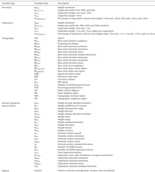
Table 2

Predictor variables used in the random forests and logistic regression classiﬁers for detection and mapping ofLigustrum sinense. LiDAR-derived variables assigned to overstory, understory, topography, and overall vegetation characteristics types while IKONOS-derived variables are optical type.

Variable type Variable name Description

Overstory HMAX Height maximum

HPCT(75–95) Height percentile 75th, 90th, and 95th VHT3 Vegetation height >5 m and≤10 m VHT4 Vegetation height >10 m

VSTRATUM(4–6) Percentage of vegetation returns in the height >10 m and≤20 m, 20 m and≤30 m, and >30 m

Understory HMIN Height minimum

HPCT(5–50) Height percentile 5th, 10th, 25th, and 50th (median) VHT1 Vegetation height >0 m and≤1 m

VHT2 Vegetation height >1 m and≤5 m (understory vegetation)

VSTRATUM(0–3) Percentage of vegetation returns in the height range >0 m and≤1 m, >1 m and≤2.5 m, and >2.5 m and≤10 m

Topography ASP Aspect

BEAR Bare earth absolute roughness BEGPD Ground point density BEIMIN Bare earth intensity minimum BEIMAX Bare earth intensity maximum BEIMEA Bare earth intensity mean

BEISD Bare earth intensity standard deviation BELmin Bare earth elevation minimum BELmax Bare earth elevation maximum BELmea Bare earth elevation mean BELR Bare earth local roughness BESLPCOSASP Bare earth slope cosine aspect BESLPSINASP Bare earth slope sine aspect DEM Digital elevation model ERR Elevation relief ratio

Crv Curvature surface

HDE Hill-shade

NLGR Number of LiDAR ground returns PGR Percentage ground return SLP Slope surface (degree) SRI Solar radiation index TMI Topographic moisture index TRI Topographic roughness index

Overall vegetation characteristics

HAAD Height average absolute deviation HCV Height coefﬁcient of variation HIQR Height interquartile range

HKUR Height kurtosis

HMAD Height median absolute deviation

HMEAN Height mean

HRNG Height range

HSD Height standard deviation

HSKE Height skewness

HTEX Height texture

HVAR Height variance

IALL Intensity surface overall IMIN Intensity surface minimum IMAX Intensity surface maximum IMEAN Intensity surface mean

ISD Intensity surface standard deviation NLR Number of LiDAR returns

NLVR Number of LiDAR vegetation returns VTVD Total vegetation density

VCTYPE Vegetation cover type (deciduous, evergreen and mixed) VIMIN Vegetation intensity minimum

VIMAX Vegetation intensity maximum VIMEAN Vegetation intensity mean

VISD Vegetation intensity standard deviation

Optical Texture Texture (contrast, homogeneity, variance, and correlation) ARVI Atmospherically resistant vegetation index

MSAVI Modiﬁed soil adjusted vegetation index IHS Hue intensity and saturation EVI Enhanced vegetation index

(5)

Fig. 2.Study system. (a) Mecklenburg County at the center of the Charlotte Metropolitan Area of North Carolina, USA, (b) the distribution of forest cover across the county with overlays of LiDAR tile index and locations of ﬁeld plots. A total of 1896 LiDAR tiles of dimension 914.40 m×914.40 m used for developing predictor variables, and (c) the extent of IKONOS coverage.

2012). To account for forest vertical structures in the analyses, we divided forest into four vertical strata (≤1 m; >1 –≤5 m; >5 –≤10 m; and >10 m) following the height range ofL. sinense. LiDAR data col-lected in the leaf-off season vary significantly both in point density and intensity values for different forest types such that contrast among different forest strata and topography is emphasized. We converted LiDAR intensity into various vegetation and topography intensity metrics. We also developed height percentile metrics to represent the proportion of vegetation below a given percentile. For example, the 99th percentile defines a measure of the maxi-mum height, whereas the remaining percentiles quantify variation in height across the vegetation profile (Jaskierniak et al., 2011).

We developed indices using a LiDAR-derived digital elevation model (DEM) to characterize moisture content and site conditions. Indices include an integrated moisture index (IMI), an elevation to relief ratio (ERR), a topographic roughness index (TRI), and a solar radiation index (SRI). An IMI with increasing values indicates increasing moisture accumulation and retention (Iverson et al., 1997). The ERR index measures the extent to which topography has been opened up by erosion (Martinuzzi et al., 2009). The TRI is a measure of variability in the landscape surface and a proxy for disturbances (Stambaugh and Guyette, 2008). The SRI affects biological processes that inﬂuence species distributions across landscapes (Keating et al., 2007). We used a three-band compos-ite dataset containing a canopy height model, a normalized digital surface model, and a differenced surface model of these two to clas-sify forested landscapes into deciduous and evergreen types (Singh

et al., 2010). We created sixty-six variables from LiDAR, consist-ing of 43 canopy and 23 topographic metrics at the county extent (Table 2). We further post-processed these metrics using a mask of vegetation cover to exclude developed land cover types from forested landscapes.

IKONOS data acquisition

(6)

IKONOS data processing

We developed fourteen spectral features, including a pan-sharpened, four-band image, a three-band hue-intensity-saturation (HIS) image, four texture images (contrast, homogeneity, variance, and correlation), and three vegetation indices: (1) enhanced vegetation index (EVI), (2) modified soil adjusted vegetation index (MSAVI), and (3) the atmospherically-resistant vegetation index (ARVI). Studies have demonstrated the efficacy of pan-sharpened imagery in the classification of forest tree species in urban areas, estimation of vegetation cover, detection of disturbance severity and canopy heterogeneity, and for under-standing the spatiotemporal distributions of forest structural and dynamic variables in the tropical forest (Carleer and Wolff, 2004; Pu, 2011). We transformed the pan-sharpened four-band image to HIS, and texture images. Texture images are useful for retrieving forest structure variables and distinguishing subtle differences in vegetation types (Franklin et al., 2001; Kayitakire et al., 2006). The EVI is suitable for detecting changes in areas of high biomass. The MSAVI distinguishes areas with a high degree of exposed soil surface. The ARVI, being less sensitive to atmospheric effects (aerosols), is useful for measuring and monitoring plant growth, vegetation cover, and biomass production. Finally, we resampled these features to 5 m resolution to match the spatial grain of the LiDAR-derived variables to facilitate comparisons.

Datasets and modeling schema

To understand the contribution of forest structure in detec-tion and mapping ofL. sinense, we categorized the LiDAR-derived variables into overstory, understory, topography, and overall vege-tation characteristics variable types and assigned IKONOS spectral features to the optical types (Table 2). We used the description of variables and their established applications in forestry-related studies for the purpose of categorization (Asner et al., 2008; Falkowski et al., 2009; Hudak et al., 2008; Jaskierniak et al., 2011; Martinuzzi et al., 2009). Using the five ‘variable types’, we devel-oped thirty-one unique combinations of models at the IKONOS experimental extent (Fig. 2c;Table 3), and then further applied the RF (Breiman, 2001) classifier to analyze relative contributions of sensors and forest landscape structures in detectionL. sinense. Finally, we compared the top performing model developed from selected predictor variables (PVs) using the RF classifier to the best parametric model developed from LR (Orka et al., 2012), and used the best overall model to map the probability ofL. sinense occur-rence across the heterogeneous county extentFig. 3.

Statistical analysis

We implemented the RF and LR classifiers in the IDL (Waske et al., 2012) and R programming environment (R Core Team, 2013), respectively. In order to account for the time lag between field data and remotely sensed data, we performed visual assessment of the field data collected prior 2012 using LiDAR canopy cover to eliminate those field plots affected by forest loss.

Traditional statistical methods do not address nonlinear complex interactions among high-dimensional remote sensing variables (Cutler et al., 2007). To overcome these limitations, we used a non-parametric RF classifier, a decision-tree-based ensemble classifier, which has proven effective in the classifica-tion of high-dimensional remote sensing and ecological data (Cutler et al., 2007; Goetz et al., 2010; Martinuzzi et al., 2009). We selected the RF classifier based on: (1) its robustness and accurate perfor-mance on complex datasets with an array of input variables (higher dimensionality) (Guo et al., 2011; Stumpf and Kerle, 2011), (2) its ability to determine significant variables in the classification, and (3) a waiver from cross-validation as it generates an internal

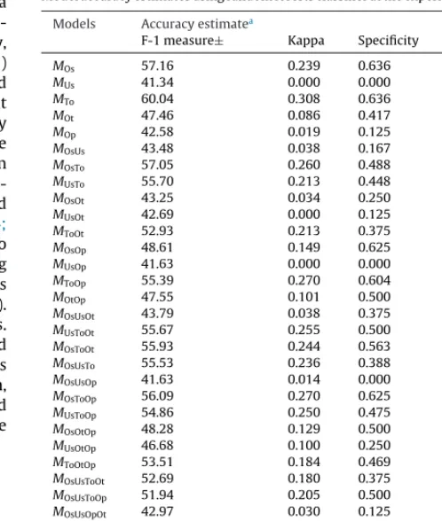
Table 3

Model accuracy estimates using random forests classiﬁer at the experimental extent.

Models Accuracy estimatea

F-1 measure± Kappa Speciﬁcity Sensitivity

MOs 57.16 0.239 0.636 0.754

MUs 41.34 0.000 0.000 0.722

MTo 60.04 0.308 0.636 0.790

MOt 47.46 0.086 0.417 0.734

MOp 42.58 0.019 0.125 0.724

MOsUs 43.48 0.038 0.167 0.724

MOsTo 57.05 0.260 0.488 0.767

MUsTo 55.70 0.213 0.448 0.742

MOsOt 43.25 0.034 0.250 0.727

MUsOt 42.69 0.000 0.125 0.725

MToOt 52.93 0.213 0.375 0.746

MOsOp 48.61 0.149 0.625 0.730

MUsOp 41.63 0.000 0.000 0.722

MToOp 55.39 0.270 0.604 0.760

MOtOp 47.55 0.101 0.500 0.733

MOsUsOt 43.79 0.038 0.375 0.739

MUsToOt 55.67 0.255 0.500 0.763

MOsToOt 55.93 0.244 0.563 0.758

MOsUsTo 55.53 0.236 0.388 0.765

MOsUsOp 41.63 0.014 0.000 0.735

MOsToOp 56.09 0.270 0.625 0.762

MUsToOp 54.86 0.250 0.475 0.758

MOsOtOp 48.28 0.129 0.500 0.733

MUsOtOp 46.68 0.100 0.250 0.728

MToOtOp 53.51 0.184 0.469 0.802

MOsUsToOt 52.69 0.180 0.375 0.751

MOsUsToOp 51.94 0.205 0.500 0.747

MOsUsOpOt 42.97 0.030 0.125 0.739

MOsToOpOt 55.68 0.238 0.531 0.749

MUsToOpOt 54.32 0.196 0.542 0.759

MALL 54.79 0.229 0.500 0.757

±F-1 measure – the harmonic mean of precision and recall.

a_{10-fold cross-validated accuracy estimate.}

unbiased estimate of test error (Cutler et al., 2007). The RF classi-fier provides estimates of variable importance in the classification to assist with reducing data dimensionality. The classifier oper-ates by growing a large number of individual decision trees from randomized subsets of training samples to maximum size without pruning, and then selecting only the best split among a random subset at each node (Falkowski et al., 2009; Prasad et al., 2006). The optimal classification is then determined by selecting the most common classification results at each node within the group of mul-tiple decision trees (Breiman, 2001). Due to the randomness, the bias of RF usually increases, but its variance also decreases due to averaging, therefore constructing the most parsimonious classifica-tion model that retains the highest classificaclassifica-tion accuracy (Cutler et al., 2007; Goetz et al., 2010). For comparison, and due to the binary nature of the output, we also applied the LR classifier to plot level datasets. This approach offers a robust discriminant function without assuming a specific distribution in the input variables.

We applied the LR classifier to analyze the presence of L. sinense, in which field-collected privet occurrence data served as the response variable and remote sensing covariates as PVs. Our selection of LR is based on its flexibility related to key statistical assumptions (linearity, normality, and homoscedasticity), and the straightforward interpretation of results based on odds ratios and statistical hypothesis testing. We modeled the logit of the presence ofL. sinenseas:

y=log_e

_P

(1−P)

=logit(P)=ˇ0+ˇ1x1+. . .+ˇkxk

whereyis a linear combination function of included PVsx1,...xk, the parameters_ˇ0+ˇ1,. . .+ˇkare the regression coefﬁcients to be

(7)

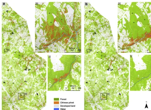
Fig. 3.The spatial distribution ofLigustrum sinensein the forest understory at experimental extent based on: (a) the top performing random forests model (F-1 accu-racy = 69.90%) developed using selected predictor variables with high variable importance, and (b) a parsimonious logistic regression model (F-1 accuaccu-racy = 54.50%).

We used the variance inflation factor (VIF)≤10 for the identifi-cation and removal of collinear PVs, and we applied the backward elimination technique by deleting one predictor variable for each iteration until no further improvement in the Akaike’s information criterion (AIC) was observed (Orka et al., 2012). Since AIC penal-izes over fitting a model, the lowest AIC value is ideal for selecting a model from a set of models for a given set of data. We used a maximized sum of specificity and sensitivity criterion (MST – max-imized sum threshold) for selecting the threshold of occurrence for L. sinensedetection. The MST is the value that maximizes the sum of specificity and sensitivity in the model, and may offer a number of cutoffs that do nearly as well. Once an optimal LR was established, we applied it to the entire dataset to produce a categorical map of presence and absence ofL. sinense.

Evaluation of model performance

We evaluated model performance by computing resubstitution and 10-fold cross-validation (k-fold CV) estimates for all models from RF and LR classifiers using F-1 measure (sensitivity, specificity, and kappa), and the area under the receiver operating character-istic curve (ROC). The area under the ROC curve ranges from 0 to 1 (none correctly classified to all correctly classified) and provides a quantitative measure of model performance. We obtained the ROC by plotting the true positive proportion of correctly predicted presences (sensitivity) on theY-axis against the false positive pro-portion of correctly predicted absences (specificity) on theX-axis. Since the RF classifier provides a reliable error estimate using data

that is randomly withheld from each iteration of tree development (the “out-of-bag” portion), an accuracy assessment using indepen-dent testing data is not required (Lawrence et al., 2006). However, for the purpose of model comparison and analytical robustness, we computed ak-fold CV by dividing the ﬁeld data into ten equal sets, where nine sets were input for training and one set for testing, and repeated this procedure ten times (Cutler et al., 2007).

Results

Understory detection and mapping performance

(8)

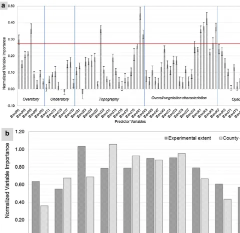
com-Fig. 4.Normalized variable importance (NVI) plot from the random forests classiﬁer showing the relative importance of each predictor variable in the model. NVI is a ratio between raw variable importance and the respective standard deviation. Higher values indicate greater contribution to the model. (a) NVI plot for the model (MALL) with all predictor variables at experimental extent, and (b) NVI plot for models developed from selected predictor variables at experimental and county extents.

Table 4

Accuracy metrics for top performing models with observed and predicted frequencies at the experimental and county extents.

Experimental extent County extent

RF LR RF

Predicted Predicted Predicted

Observed Presence Absence % Correct Presence Absence % Correct Presence Absence % Correct

Presence 11 9 55.00 15 20 42.90 92 31 74.80

Absence 0 61 100.00 5 41 89.10 35 187 84.20

Overall % correct 88.89 69.14 80.87

Accuracy estimates

F-1 measures: 71.00 F-1 measures: 54.50 F-1 measures: 73.60

Kappa: 0.648 Kappa: 0.337 Kappa: 0.586

Sensitivity: 1.000 Sensitivity: 0.750 Sensitivity: 0.724

Specificity: 0.871 Specificity: 0.672 Specificity: 0.858

AUC: 0.936 AUC: 0.787 AUC: 0.791

10-fold cross-validation

F-1 measures: 61.55 F-1 measures: 53.30 F-1 measures: 67.37

Kappa: 0.537 Kappa: 0.331 Kappa: 0.547

(9)

Fig. 5.Logistic regression results at the experimental extent. (a) A maximized sum of sensitivity and speciﬁcity criterion for selecting the threshold of occurrence, and (b) the receiver operating characteristic (ROC) curve for the logistic regression model. The stair-stepped line represents the ROC curve (area under the curve, 0.787 [95% CI, 0.74–0.83]).

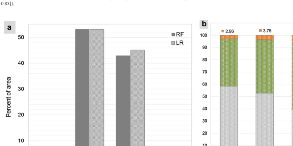
Fig. 6.EstimatedLigustrum sinensecover (% of area) in the forest understory at experimental extent. (a) The distribution ofL. sinenseand other land covers derived from top performing random forests (RF) and logistic regression (LR) models, and (b) the proportions ofL. sinensecover along the urban–rural gradient.

bination of variable type using the RF classifier, respectivelyFig. 5 (Table 4). The F-1 estimate between resubstitution andk-fold CV varies on average 7.84% using the RF classifier compared to 1.2% using LR. The RF classifier predicted nearly three times the area ofL. sinensespread in the understory of forests at the experimen-tal extent compared to the LR classifier (Fig. 6a). The ratio ofL. sinenseto forest cover is nearly consistent across urban-rural gra-dients. However, the ratio ofL. sinenseto developed land cover in rural areas is 71% higher than in suburban areas, and 140% higher

(10)

Fig. 7.The spatial distribution ofLigustrum sinenseusing the random forests classiﬁer in the forest understory at the county extent.

Relative contribution of IKONOS imagery and LiDAR data

The F-1 and kappa estimates obtained from RF classification of optical PVs were only 1.25% and 1.9% higher, respectively, than the understory model, and contributed only marginally to improvements in overall accuracy estimates when combined with overall vegetation characteristics and understory PVs (Table 3). However, the IKONOS-derived PVs when analyzed together with the other LiDAR PVs did not improve classification accuracy esti-mates of detection and mappingL. sinense. Among the optical PVs, texture contributed slightly to improved detection when combined with overall vegetation characteristics while no other optical PVs were significant in the top performing RF and LR analysis.

Contributions of forest landscape structures

The topography PVs alone produced the highest accuracy esti-mates and contributed more to detection ofL. sinensethan other variable types across all models created by the combination of vari-able type using the RF classiﬁer at the experimental extent. The F-1 estimate was 11.4% higher than average estimates obtained from other variable types alone, followed by overstory and over-all vegetation characteristics (Table 3). Gains in accuracies did not improve with increasing numbers of variable types except for a slight improvement of_≥0.2 kappa with the topography PVs. How-ever, the RF variable importance plot of theMALL model (Fig. 4a)

produced a higher number of PVs from overall vegetation

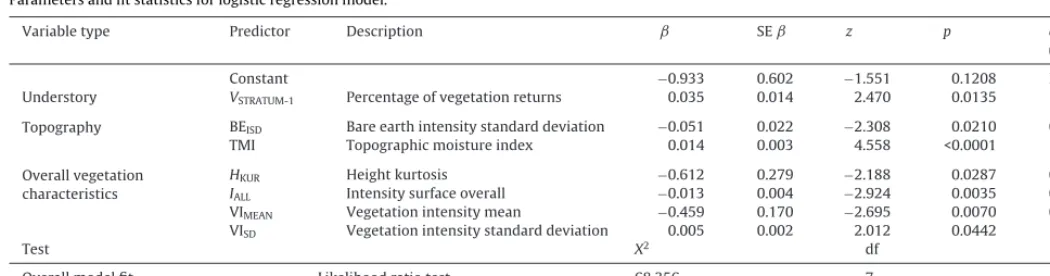
charac-teristics contributing in the overall accuracy estimates followed by the topography and overstory variable types. The LR analysis also identiﬁed similar sets of signiﬁcant variable types with the excep-tion of understory (VSTRATUM−1) (Table 5). Two PVs: TMI and VISD,

are significant in both the top performing models from RF classi-fier and model from the LR classiclassi-fier. LiDAR intensity-derived forest landscape variables (VIMEAN/VIMAXand VIMIN) contributed in both

top performing RF and LR models. However, the lower performance suggests that the LR classiﬁer was unable to address adequately some nonlinear structure for matching or higher accuracy esti-mates. The LR classiﬁer revealed the magnitude and direction of PVs’ contribution in the detection ofL. sinense. Examination of the RF variable importance plots showed that in addition to the TMI, three PVs (topographic roughness index, vegetation density and forest cover types) contributed considerably to improved detection with higher accuracy estimates at both experimental and county extents (Fig. 4b).

Large-area assessment of L. sinense

(11)

Table 5

Parameters and ﬁt statistics for logistic regression model.

Variable type Predictor Description ˇ SEˇ z p eˇ

(odds ratio)

Constant −0.933 0.602 −1.551 0.1208 NA

Understory VSTRATUM-1 Percentage of vegetation returns 0.035 0.014 2.470 0.0135 1.036

Topography BEISD Bare earth intensity standard deviation −0.051 0.022 −2.308 0.0210 0.950

TMI Topographic moisture index 0.014 0.003 4.558 <0.0001 1.014

Overall vegetation characteristics

HKUR Height kurtosis −0.612 0.279 −2.188 0.0287 0.542

IALL Intensity surface overall −0.013 0.004 −2.924 0.0035 0.987

VIMEAN Vegetation intensity mean −0.459 0.170 −2.695 0.0070 0.631

VISD Vegetation intensity standard deviation 0.005 0.002 2.012 0.0442 1.005

Test X2 _df _P

Overall model ﬁt Likelihood ratio test 68.356 7 <0.0001

Wald test 13.900 2 0.0009

sensitivity and speciﬁcity, which suggests an improved prediction. The variable importance plot indicated TMI as the most signiﬁcant PV for large-area assessment ofL. sinense, followed by VCTYPE, TRI,

and vegetation density (Fig. 4b). The analysis of LiDAR PVs and the RF classiﬁer with the county level ﬁeld data mapped the spatial distribution ofL. sinensethat occupies 5.95% of forest understory, predominantly in drainage ways and lowland areas of forested landscapes along urban–rural gradients in the county (Fig. 7).

Discussion

Regional assessment of understory invasions requires an approach that overcomes the complicacies of spatial and vertical heterogeneity of forested landscapes, and utilizes structural and spectral remote sensing data in a coherent manner. In this study, we found that structural and spectral data from LiDAR can be used to detectL. sinenseover large areas with greater accuracy than either using multispectral IKONOS data alone or the combination of pre-dictors derived from LiDAR and IKONOS. We obtained high accuracy estimates using the RF classiﬁer with selected LiDAR PVs at both the experimental and county extents (Table 4). Topographic attributes, including TMI and TRI, together with vegetation height and LiDAR’s spectral metrics contributed the most in the detection ofL. sinense, regardless of the classiﬁer used.

Contrary to our expectations, high resolution IKONOS did not contribute significantly to the detection ofL. sinense, revealing the limited ability of spectral remote sensing to unravel vertical struc-ture of heterotypic forest stands. The ineffectiveness of IKONOS in the detection ofL. sinensecould be due to cumulative or individ-ual constraints in spectral, spatial, and temporal resolutions. The heterogeneity of forest strata is responsible for the mixed spectral response resulting in scale-dependent variance. This could be fur-ther complicated with an off-nadir effect of tall trees on understory vegetation as found in (Hsieh et al., 2001) and (Myeong et al., 2006). Decreasing the spatial resolution of IKONOS spectral features to 5 m for spatial consistency across the analysis and the uneven geo-registration between IKONOS and LiDAR may have also contributed to poor results (Nelson et al., 2006). A time lag in acquisition (a tem-poral gap) may also contribute to problematic integration of the two remote sensing data sources, which is also the case in this study. Accurate detection of understory plant invasions is scale (scale of the study) and data dependent, considering the types of data ana-lyzed, the existing data dimensionality and nonlinearity, and the data acquisition period. The choice of classification techniques also influenced computational efficiency and detection success. More-over, detection success is most dependent upon the characteristics of forested landscapes, including physiology of invasive shrubs and the host environment (Chastain and Townsend, 2007; Resasco et al., 2007).

Our approach of dividing PVs from LiDAR into variable types rep-resenting characteristics of forest structure and forested landscapes added a new element into the design of our analytical frame-work. The RF accuracy estimates of models based on LiDAR-derived variable type combinations (Table 3) illustrate the significance of forest structure and landscape characteristics and their contribu-tion in deteccontribu-tion and mappingL. sinense. The topography variables contributed the most with improved detection once combined with overall vegetation characteristics, and overstory using the RF classifier. Among our broad variable types, topographic mois-ture, roughness, vegetation height, and vegetation intensity profile were key variables in the RF and LR models at both extents (Fig. 4a and b,Table 4). Topographic moisture and roughness play impor-tant roles in the growth and distribution ofL. sinensein riparian forests of the southeastern United States (Hudson et al., 2013; Wang and Grant, 2012), therefore, the influence of these variables in the analysis is not surprising. The significance of vegetation height, density, and intensity profiles variables supports our con-cept that physiological characteristics ofL. sinenseare the most suitable for LiDAR-based detection. The prominence of vegeta-tion density and intensity variables in our analysis also suggests that LiDAR with higher point-density, acquired in the peak of senescence period, can improve detection and mapping by pro-viding distinct spectral contrast and vegetation densities between deciduous and compact evergreen understory, which corroborates the findings ofStraatsma and Middelkoop (2007).

Our k-fold CV of model performance helped minimize the over-fitting tendency of the RF classifier and provided a direct comparison between RF and LR models. The RF classifier outper-formed the LR classifier using the same set of selected PVs.Cutler et al. (2007)observed higher performance using the RF classifier when there were strong interactions among the PVs. RF’s abil-ity to model complex interactions among PVs perhaps addresses the complicated interactions of LiDAR-derived PVs in the top performing model and explains the better performance of RF classifier. The common PVs in both classifiers, for example, TMI and VISD, and the marginal difference in AUC value suggests that

(12)

advantage over LR. In general, a higher number of presence data in the model poses a challenge of overestimation. On the contrary, due to a higher number of absence data, more than twice the presence data at both extents, we expect that neither classiﬁer overestimated the spatial distribution ofL. sinense.

We identified two primary sources of error in the overestima-tion of ‘sensitivities’ in models: (1) the presence of other evergreen understory shrubs, and (2) the use of field plots containing a fewer number of seedlings, juveniles, and matures as presence in the classifiers. However, the effects of higher evergreen shrub coverage and plots with sparserL. sinenseplants on detection and mapping are matters for further analysis. Other technical issues influencing accuracy estimates were GPS positional errors from the fieldwork, loss of information during data conversion (e.g., float to integer), and the quality of LiDAR data and derived variables at regional extents, including gaps between LiDAR tiles and non-calibrated LiDAR intensity. Computational challenges that arose due to large data volumes associated with the large-area LiDAR application sug-gest that we need to explore data reduction techniques and optimal resolutions for detection and mapping of understory plant invaders. We observed little difference in accuracy estimates when imple-menting the RF classifier at the experimental and county extents, with only slightly reduced variability between resubstitution andk -fold CV at the county extent. This reduced variability is attributable to the larger amounts of field data at the county extent. However, similar accuracy estimates at both extents suggests the suitabil-ity of the RF classifier when less field data is available, which is consistent with research presented by Martinuzzi et al. (2009). County-level analyses showed that TMI and vegetation cover types – deciduous and evergreen – (VCTYPE) are the most important

variables for predicting the distribution ofL. sinenseat that scale. Application of the RF classifier at the county extent prompted two methodological avenues for future research: (1) to analyze LiDAR-derived PVs with spatial resolution matching the field plot size (i.e., 10 m_×10 m) to enhance data handling and computational effi-ciency while providing sufficient accuracy estimates, and (2) to measure the variability in accuracy estimates when using other evergreen understory invasive species found in the field plots. Ultimately, using county-level field data with the RF classifier is suitable for large-area assessment ofL. sinense, and this approach can be applied to other local and regional sites.

Conclusions

Successful management of native biodiversity and ecosystem services at regional scales requires methodological advances in the application of remote sensing technologies aiming to accu-rately quantify the spatial distribution of invasive species. Our results suggest that LiDAR data provides: (1) adequate informa-tion for accurately detecting and mapping the spatial distribuinforma-tion of the understory invasiveL. sinenseover large urbanizing regions, and (2) improved results as compared to the analysis of IKONOS optical imagery. The topography variables (TMI + TRI), when com-bined with overall vegetation characteristics (density + spectral) and overstory (height), produced the highest accuracy estimates. These findings highlight the significance of the structural and spectral characteristics of LiDAR for quantifying the landscape-level topographic, forest stand, and physical and structural plant attributes used for detecting and mapping the distribution ofL. sinense. LiDAR intensity-derived variables were significant in the successful detection and mapping ofL. sinense, emphasizes the importance of the spectral attributes of LiDAR data for assessing understory invasives. This research demonstrates how categorizing LiDAR-derived variables into variable types representing overstory and understory forest structure and topography contributed to

our understanding of the forest and landscape characteristics that inﬂuence the distribution, growth, and detection ofL. sinense. Our study suggests an even distribution ofL. sinensein forests along the urban–rural gradients of Mecklenburg County, NC, found predom-inantly in drainage ways, lowlands, and disturbed areas of forested landscapes as observed during ﬁeldwork. This research further highlights the importance of LiDAR data acquisition during the leaf-off season for mappingL. sinense. Our methodological frame-work addresses data complexities, including multidimensionality and nonlinearity in multisource data, and provides a generalized approach for rapid assessments ofL. sinensein forested landscapes over large urbanizing regions to support development and imple-mentation of management plans for conserving native biodiversity.

Acknowledgements

This research was supported by the National Science Foundation ULTRA-Ex program (BCS-0949170), Renaissance Computing Insti-tute (RENCI), Garden Club of America (GCA) Zone VI fellowship in urban forestry, Casey Trees Endowment Fund, and the AAG (Asso-ciation of American Geographers) Dissertation Research grants. We express sincere thanks to Drs. Marguerite Madden, Hugh Devine, Stacy Nelson, and Helena Mitasova for their comments and feed-back for shaping the research and manuscript. We thank S. Gagné (UNC Charlotte) for providing IKONOS data. We also thank fellow graduate students from the Center for Geospatial Analytics, North Carolina State University, for their comments and feedback on the manuscript.

References

Andrew, M.E., Ustin, S.L., 2009. Habitat suitability modelling of an invasive plant with advanced remote sensing data. Divers. Distrib. 15, 627–640.

Asner, G.P., Vitousek, P.M., 2005. Remote analysis of biological invasion and biogeochemical change. Proc. Natl. Acad. Sci. U. S. A. 102, 4383–4386. Asner, G.P., Knapp, D.E., Kennedy-Bowdoin, T., Jones, M.O., Martin, R.E., Boardman,

J., Hughes, R.F., 2008. Invasive species detection in Hawaiian rainforests using airborne imaging spectroscopy and LiDAR. Remote Sens. Environ. 112, 1942–1955.

BCAL LiDAR Tools (2013). Idaho State University, Department of Geosciences. In. Boise, Idaho: Boise Center Aerospace Laboratory (BCAL).

Becker, R., Zmijewski, K., Crail, T., 2013. Seeing the forest for the invasives: mapping buckthorn in the Oak openings. Biol. Invasions 15, 315–326. Breiman, L., 2001. Random forests. Mach. Learn. 45, 5–32.

Brown, C.E., Pezeshki, S.R., 2000. A study on waterlogging as a potential tool to controlLigustrum sinensepopulations in western Tennessee. Wetlands 20, 429–437.

Carleer, A., Wolff, E., 2004. Exploitation of very high resolution satellite data for tree species identiﬁcation. Photogramm. Eng. Remote Sens. 70, 135–140. Chastain, R.A., Townsend, P.A., 2007. Use of landsat ETM and topographic data to

characterize evergreen understory communities in appalachian deciduous forests. Photogramm. Eng. Remote Sens. 73, 563–575.

Cutler, D.R., Edwards, T.C., Beard, K.H., Cutler, A., Hess, K.T., 2007. Random forests for classiﬁcation in ecology. Ecology 88, 2783–2792.

EDDMapS, 2014. Early Detection Distribution Mapping System. In. The University of Georgia – Center for Invasive Species and Ecosystem Health. The University of Georgia.

Estes, L.D., Reillo, P.R., Mwangi, A.G., Okin, G.S., Shugart, H.H., 2010. Remote sensing of structural complexity indices for habitat and species distribution modeling. Remote Sens. Environ. 114, 792–804.

Estornell, J., Ruiz, L.A., Velazquez-Marti, B., Fernandez-Sarria, A., 2011. Estimation of shrub biomass by airborne LiDAR data in small forest stands. For. Ecol. Manage. 262, 1697–1703.

Falkowski, M.J., Evans, J.S., Martinuzzi, S., Gessler, P.E., Hudak, A.T., 2009. Characterizing forest succession with lidar data: an evaluation for the Inland Northwest USA. Remote Sens. Environ. 113, 946–956.

Faulkner, J.L., Clebsch, E.E.C., Sanders, W.L., 1989. Use of Prescribed Burning for Managing Natural and Historic Resources in Chickamauga and Chattanooga National Military Park USA. Environ. Manage. 13, 603–612.

Franklin, S.E., Wulder, M.A., Gerylo, G.R., 2001. Texture analysis of IKONOS panchromatic data for Douglas-ﬁr forest age class separability in British Columbia. Int. J. Remote Sens. 22, 2627–2632.

(13)

Goetz, S.J., Steinberg, D., Betts, M.G., Holmes, R.T., Doran, P.J., Dubayah, R., Hofton, M., 2010. Lidar remote sensing variables predict breeding habitat of a Neotropical migrant bird. Ecology 91, 1569–1576.

Greene, B.T., Blossey, B., 2012. Lost in the weeds:Ligustrum sinensereduces native plant growth and survival. Biol. Invasions 14, 139–150.

Guo, L., Chehata, N., Mallet, C., Boukir, S., 2011. Relevance of airborne lidar and multispectral image data for urban scene classiﬁcation using random forests. ISPRS J. Photogramm. Remote Sens. 66, 56–66.

Hanula, J.L., Horn, S., Taylor, J.W., 2009. Chinese privet (Ligustrum sinense) removal and its effect on native plant communities of Riparian Forests. Invasive Plant Sci. Manage. 2, 292–300.

Hestir, E.L., Khanna, S., Andrew, M.E., Santos, M.J., Viers, J.H., Greenberg, J.A., Rajapakse, S.S., Ustin, S.L., 2008. Identiﬁcation of invasive vegetation using hyperspectral remote sensing in the California Delta ecosystem. Remote Sens. Environ. 112, 4034–4047.

Homolova, L., Maenovsky, Z., Clevers, J.G.P.W., Garcia-Santos, G., Schaeprnan, M.E., 2013. Review of optical-based remote sensing for plant trait mapping. Ecol. Complex. 15, 1–16.

Hsieh, P.F., Lee, L.C., Chen, N.Y., 2001. Effect of spatial resolution on classiﬁcation errors of pure and mixed pixels in remote sensing. IEEE Trans. Geosci. Remote Sens. 39, 2657–2663.

Huang, C.-Y., Asner, G.P., 2009. Applications of remote sensing to alien invasive plant studies. Sensors 9, 4869–4889.

Hudak, A.T., Crookston, N.L., Evans, J.S., Hall, D.E., Falkowski, M.J., 2008. Nearest neighbor imputation of species-level, plot-scale forest structure attributes from LiDAR data. Remote Sens. Environ. 112, 2232–2245.

Hudson, J.R., Hanula, J.L., Horn, S., 2013. Removing Chinese privet from riparian forests still beneﬁts pollinators ﬁve years later. Biol. Conserv. 167, 355–362.

Iverson, L.R., Dale, M.E., Scott, C.T., Prasad, A., 1997. A GIS-derived integrated moisture index to predict forest composition and productivity of Ohio forests (USA). Landscape Ecol. 12, 331–348.

Jaskierniak, D., Lane, P.N.J., Robinson, A., Lucieer, A., 2011. Extracting LiDAR indices to characterise multilayered forest structure using mixture distribution functions. Remote Sens. Environ. 115, 573–585.

Kayitakire, F., Hamel, C., Defourny, P., 2006. Retrieving forest structure variables based on image texture analysis and IKONOS-2 imagery. Remote Sens. Environ. 102, 390–401.

Keating, K.A., Gogan, P.J.P., Vore, J.M., Irby, L.R., 2007. A simple solar radiation index for wildlife habitat studies. J. Wildl. Manage. 71, 1344–1348.

Laba, M., Downs, R., Smith, S., Welsh, S., Neider, C., White, S., Richmond, M., Philpot, W., Baveye, P., 2008. Mapping invasive wetland plants in the Hudson River National Estuarine Research Reserve using quickbird satellite imagery. Remote Sens. Environ. 112, 286–300.

Langeland, K.A., Burks, K.C., 1998. In: Langeland, K.A., Burks, K.C. (Eds.), Identiﬁcation and Biology of Non-Native Plants in Florida’s Natural Areas. University of Florida, Gainesville, p. 165.

Lawrence, R.L., Wood, S.D., Sheley, R.L., 2006. Mapping invasive plants using hyperspectral imagery and Breiman–Cutler classiﬁcations (Random forest). Remote Sens. Environ. 100, 356–362.

Linderman, M., Liu, J., Qi, J., An, L., Ouyang, Z., Yang, J., Tan, Y., 2004. Using artiﬁcial neural networks to map the spatial distribution of understorey bamboo from remote sensing data. Int. J. Remote Sens. 25, 1685–1700.

Martinuzzi, S., Vierling, L.A., Gould, W.A., Falkowski, M.J., Evans, J.S., Hudak, A.T., Vierling, K.T., 2009. Mapping snags and understory shrubs for a LiDAR-based assessment of wildlife habitat suitability. Remote Sens. Environ. 113, 2533–2546.

Merriam, R.W., Feil, E., 2002. The potential impact of an introduced shrub on native plant diversity and forest regeneration. Biol. Invasions 4, 369–373.

Miller, J.H., Chambliss, E.B., Oswalt, C.M., 2008. Maps of occupation and estimates of acres covered by nonnative invasive plants in southern forests using SRS FIA data. In.

Mutlu, M., Popescu, S.C., Stripling, C., Spencer, T., 2008. Mapping surface fuel models using lidar and multispectral data fusion for ﬁre behavior. Remote Sens. Environ. 112, 274–285.

Myeong, S., Nowak, D.J., Duggin, M.J., 2006. A temporal analysis of urban forest carbon storage using remote sensing. Remote Sens. Environ. 101, 277–282. Nelson, S.A.C., Cheruvelil, K.S., Soranno, P.A., 2006. Satellite remote sensing of

freshwater macrophytes and the inﬂuence of water clarity. Aquat. Bot. 85, 289–298.

Orka, H.O., Wulder, M.A., Gobakken, T., Naesset, E., 2012. Subalpine zone delineation using LiDAR and Landsat imagery. Remote Sens. Environ. 119, 11–20.

Popescu, S.C., Wynne, R.H., Scrivani, J.A., 2004. Fusion of small-footprint lidar and multispectral data to estimate plot-level volume and biomass in deciduous and pine forests in Virginia USA. For. Sci. 50, 551–565.

Prasad, A.M., Iverson, L.R., Liaw, A., 2006. Newer classiﬁcation and regression tree techniques: bagging and random forests for ecological prediction. Ecosystems 9, 181–199.

Pu, R.L., 2011. Mapping urban forest tree species using IKONOS imagery: preliminary results. Environ. Monit. Assess. 172, 199–214.

R Core Team (2013). R: A Language and Environment for Statistical Computing. In. Vienna, Austria: R Foundation for Statistical Computing.

Resasco, J., Hale, A.N., Henry, M.C., Gorchov, D.L., 2007. Detecting an invasive shrub in a deciduous forest understory using late-fall Landsat sensor imagery. Int. J. Remote Sens. 28, 3739–3745.

Royo, A.A., Carson, W.P., 2006. On the formation of dense understory layers in forests worldwide: consequences and implications for forest dynamics, biodiversity and succession. Can. J. For. Res. 36, 1345–1362.

Rushton, S.P., Ormerod, S.J., Kerby, G., 2004. New paradigms for modelling species distributions? J. Appl. Ecol. 41, 193–200.

Simberloff, D., Martin, J.L., Genovesi, P., Maris, V., Wardle, D.A., Aronson, J., Courchamp, F., Galil, B., Garcia-Berthou, E., Pascal, M., Pysek, P., Sousa, R., Tabacchi, E., Vila, M., 2013. Impacts of biological invasions: what’s what and the way forward. Trends Ecol. Evol. 28, 58–66.

Singh, K.K., Vogler, J.B., Meng, Q., Meentemeyer, R.K., 2010. Mapping land use patterns in an urbanizing landscape using LiDAR intensity data. In: In, Optical Remote Sensing of the Environment. Optical Society of America, Tucson, AZ, pp. OMC2.

Singh, K.K., Vogler, J.B., Shoemaker, D.A., Meentemeyer, R.K., 2012. LiDAR-Landsat data fusion for large-area assessment of urban land cover: balancing spatial resolution data volume and mapping accuracy. ISPRS J. Photogramm. Remote Sens. 74, 110–121.

Singh, K.K., Chen, G., McCarter, J.B., Meentemeyer, R.K., 2015. Effect of LiDAR point density and landscape context on estimates of urban forest biomass. ISPRS J. Photogramm. Remote Sens., In Press

http://dx.doi.org/10.1016/j.isprsjprs.2014.12.021

Stambaugh, M.C., Guyette, R.P., 2008. Predicting spatio-temporal variability in ﬁre return intervals using a topographic roughness index. For. Ecol. Manage. 254, 463–473.

Straatsma, M., Middelkoop, H., 2007. Extracting structural characteristics of herbaceous ﬂoodplain vegetation under leaf-off conditions using airborne laser scanner data. Int. J. Remote Sens. 28, 2447–2467.

Stumpf, A., Kerle, N., 2011. Object-oriented mapping of landslides using random forests. Remote Sens. Environ. 115, 2564–2577.

Tuanmu, M.N., Vina, A., Bearer, S., Xu, W.H., Ouyang, Z.Y., Zhang, H.M., Liu, J.G., 2010. Mapping understory vegetation using phenological characteristics derived from remotely sensed data. Remote Sens. Environ. 114, 1833–1844.

USFWS, 1991. Endangered and threatened wildlife and plants: determination of

Helianthus schweinitzii(Schweinitz’s sunﬂower) to be an endangered species. Fed. Regist. 56, 21087–21091.

Ulyshen, M.D., Horn, S., Hanula, J.L., 2010. Response of beetles (Coleoptera) at three heights to the experimental removal of an invasive shrub, Chinese privet (Ligustrum sinense) from ﬂoodplain forests. Biol. Invasions 12, 1573–1579. Wang, H.H., Grant, W.E., 2012. Determinants of Chinese and European privet

(Ligustrum sinenseandLigustrum vulgare) invasion and likelihood of further invasion in southern U.S. forestlands. Invasive Plant Sci. Manage. 5, 454–463.

Wang, T.J., Skidmore, A.K., Toxopeus, A.G., 2009. Improved understorey bamboo cover mapping using a novel hybrid neural network and expert system. Int. J. Remote Sens. 30, 965–981.

Waske, B., van der Linden, S., Oldenburg, C., Jakimow, B., Rabe, A., Hostert, P., 2012. imageRF – a user-oriented implementation for remote sensing image analysis with random forests. Environ. Model. Software 35, 192–193.

Wilfong, B.N., Gorchov, D.L., Henry, M.C., 2009. Detecting an invasive shrub in deciduous forest understories using remote sensing. Weed Sci. 57, 512–520. Wing, B.M., Ritchie, M.W., Boston, K., Cohen, W.B., Gitelman, A., Olsen, M.J., 2012.