Queries: Properties and Algorithms
Rong Huang1, Rada Chirkova2, and Yahya Fathi1
1 Operations Research Program, NC State University, Raleigh, NC 27695,
{rhuang,fathi}@ncsu.edu
2 Computer Science Department, NC State University, Raleigh, NC 27695,
Abstract. Materialized views are widely used in many data-intensive systems to accelerate the processing of complex data-analysis queries. In this paper we study the following deterministic view selection problem
(DV S): Given a collection of queries on a given star-schema data ware-house, and a storage limit on the total size of the views that we may materialize, select a collection of views to materialize so as to minimize the total evaluation cost of the given queries. We characterize the struc-tural properties of potentially beneficial views in relation to the given queries in the context of an integer programming (IP) model of this problem. We propose a procedure to effectively prune the search space of potentially beneficial views and reduce the size of the corresponding IP model, which enable us to obtain optimal solutions of realistic-size instances of problem DV S. We also present two heuristic methods to further reduce the search space of views to efficiently obtain competitive inexact solutions for large-size instances of the problem. We evaluate the effectiveness of our proposed techniques through a comprehensive computational study. We also present a computational experiment to compare our methods to those proposed in Asgharzadeh et al. [3, 4]. We show that our approaches compare favorably with those in [3,4]. In addi-tion, our proposed techniques in this paper are complementary to those in [3, 4] and can be employed either separately or in conjunction with these earlier techniques.
1
Introduction
please see [20] and references therein. As such, materialized views with group-ing and aggregation may be especially attractive for evaluatgroup-ing data-analysis queries, because the relations for such views store in compact form the results of (typically expensive) preprocessing of large amounts of data.
Consider an illustration. Large retailer companies, such as Sears in the USA, maintain significant-size databases storing information about ongoing point-of-sale transactions (Pos). For accounting, reporting, and business-intelligence pur-poses, Sears database system undergoes periodic runs of data-analysis queries on the stored information, including the queries for automatically or manually generated daily, weekly, or monthly summary reports. For instance, the query workload contains the following SQL queries Q1and Q2. Q1 asks for the total sales per item category per customer type in December 2011. Q2 asks for the maximum sales per item category per store in December after 2005. 3
Q1: SELECT itemCategory, custType, SUM (amount) FROM Pos WHERE month = ‘December’ AND year = 2011 GROUP BY itemCategory, custType;
Q2: SELECT itemCategory, storeID, MAX (amount)
FROM Pos WHERE month = ‘December’ AND year > 2005 GROUP BY itemCategory, storeID;
The following view V, which stores total sales (V1amt) and maximum sales (V2amt) per item category per customer type per store per month per year, can be used to provide the exact answers to bothQ1andQ2.
V: SELECT itemCategory, custType, storeID, SUM (amount) AS V1amt, MAX (amount) AS V2amt
FROM Pos GROUP BY itemCategory, custType, storeID, month, year; The cost of evaluation of queries Q1 and Q2 can be reduced significantly by using viewV, as it avoids accessing a large amount of irrelevant data in the base relation (Pos).
Ideally in the data-analysis setting, in order to maximize the efficiency of query processing, all the “beneficial views” would be pre-computed and stored (materialized). However, the amount of storage space and computational con-straints limit the beneficial views that can be materialized. Naturally, the prob-lem of selecting an appropriate collection of materialized views has to be ad-dressed in the context of the objectives and limitations of that setting. This problem is commonly known as the View Selection Problem. In recent years a number of researchers have addressed the subject and developed exact and inexact methods for solving the view-selection problem in a deterministic envi-ronment where all queries are assumed to be known and given in advance. See, 3 To greatly simplify this example, we assume that the data in the Sears database are
for instance, [3–5, 12, 15]. In this paper we build on the work of Asgharzadeh et al. [3, 4] who solve the problem under a space limit on the materialized views, and propose new techniques for solving the problem which are more effective than the existing methods. The techniques we propose in this paper for reducing the search space of views are complementary to those proposed in [3,4] and can be employed either separately or in conjunction with those in [3, 4].
The specific contribution of this paper is as follows:
1. We study the structure and properties of views and queries in the integer-programming model for the view-selection problem. We develop an algorithm that effectively reduces the search space of potentially beneficial views in this IP model, and obtain a smaller IP model whose solution is guaranteed to be optimal for the original problem.
2. We present a computational experiment on our smaller IP model, and discuss the scalability of this model. The size of the IP model is significantly reduced, so that for realistic-size instances of the problem this IP model can be solved efficiently by a commercial IP solver, such as CPLEX [16].
3. We define the cost-benefit ratio of each view which is a measure of effective-nessof the view with respect to the given collection of queries. We conduct a theoretical analysis of the properties of the cost-benefit ratio. Based on these properties, we develop two heuristic methods to further reduce the size of the resulting IP models to manageable levels, although we can no longer guarantee that the resulting solution is optimal for the original problem. 4. We present a computational experiment to evaluate the effectiveness of the
proposed heuristic methods. The size of the models are significantly reduced to a manageable level even for large-size instances, so that these models can be solved by CPLEX to provide close optimal solution for the original problem. We compare the performance of our proposed heuristic methods with the heuristic algorithms in [3, 4].
The remainder of this paper is organized as follows. We review related work in Section 1.1. In Section 2, we discuss the formulation and settings for the deterministic view-selection problem, and introduce the IP model. In Section 3, we discuss the properties of the queries and views. In Section 4 we propose (exact) approaches to reduce the size of the IP model, while maintaining that the resulting optimal solution of the IP model is also optimal for the original problem. Section 5 contains the computational results for the exact approaches. In Section 6 we propose (heuristic) methods for further reducing the size of resulting IP model, but we no longer guarantee optimality. In Section 7 we conduct a computational experiment for the heuristic methods and report our findings. Finally, Section 8 contains a few concluding remarks.
1.1 Related work
design goals of the problem). One line of the past research consider the view-selection under a deterministic environment where all queries are assumed to be known and given in advance. Numerous algorithms are proposed for this problem (see [14] for a survey). Significant work has also been done on index selection in such settings, both on its own and alongside view selection, please see [1,2,6,7,10]. Notable work including [13,15] considers greedy algorithms for efficiently selecting views (with or without) indexes in a generalization of the OLAP setting. Unfortunately, the paper [18] disproves the strong performance bounds of these algorithms, by showing that the underlying approach of [15] cannot provide the stated worst-case performance ratios unless P=NP.
Considerable work including [3–5,21,25] has been done in the open literature that employ integer linear programming (ILP) models to obtain the optimal se-lection of derived data for query processing. In particular, a line of past work [3–5] has focused on formal approaches to selection of views (with or without indexes) to minimize the cost of query processing under storage-space constraint. The results of that work are scalable to realistically large numbers of queries and views, and compare beneficially with several other approaches in the literature including [2, 15, 17], please see [3–5] for the details. In this paper our proposed techniques and IP models are complementary to those proposed in [3, 4] (see Section 2.2 for an overview), and can be employed either separately or in con-junction with these earlier techniques.
2
Background
In this section, we define the scope of the view-selection problem that we con-sider, that is, the type of the database, queries and views. We also briefly review the models and algorithms in [3,4], based on which, we build our proposed models and methods.
2.1 Problem specification
We consider a star-schema data warehouse [8, 9] with a single fact table and several dimension tables. We assume that all the views to be materialized are defined, with grouping and aggregation but without selection, on the relation (which we call theraw-data view) that is the result of the “star-schema join” [19] of all the relations in the schema. We can show formally that for each query posed on the original database, the query can be rewritten equivalently into a query posed on the raw-data view. Using this formal result, in the remainder of the paper we assume that all the queries in the workloads that we consider are posed on the relevant raw-data view. In this context, we consider the evaluation costs of answering unnested select-project-join queries with grouping and aggregation using unindexed materialized views, such that each query can be evaluated using just one view and no other data. (This setting is the same as in [4,15,17,22,25].) A queryqcan be answered using a viewvonly if the set of grouping attributes
those attributes in theWHEREclause ofq that are compared with constants. We
usevto represent both a view and the collection of grouping attributes for that
view, and we use q to represent both a query and the collection of attributes
in theGROUP BY clause of that query plus those attributes in theWHERE clause of the query that are compared with constants. It follows that queryq can be
answered by view v if and only if q ⊆ v. To evaluate a query using a given
view (if this view can indeed be used to answer the query) we have to scan all rows of the view. Hence the corresponding evaluation cost is equal to the size of the view itself; similar cost calculation is used in [4, 15, 17, 22, 25]. One way to estimate the view sizes in practice, as suggested in the literature, is by getting a relatively small-size sample of the raw-data view and by then evaluating the view definitions on that table, with a subsequent scaleup of the sizes of the resulting relations. We useaito denote the size of each viewvi in the problem input. We
also use the parameterdij to denote the evaluation cost of answering query qj
using viewvi. It follows that for each query qj we havedij =ai ifqj ⊆vi, and
we setdij = +∞otherwise, implying thatqj cannot be answered by viewvi.
We consider the following problem, which we call the Deterministic View-Selection (DV S) problem: Given a collectionQof queries on a given star-schema
data warehouseD, and a storage limit b on the total size of the views that we
may materialize, select a collection of views to materialize so as to minimize the total evaluation cost of the given queries.
The search space of views that we consider for a given problem DV S is
theview lattice introduced by Harinarayan et al. in [15], which includes all the views defined on the raw-data table, such that each view has aggregation on all the attributes aggregated in the input queries. In the view lattice, each node represents a view, and a directed edge from nodev1 to nodev2 implies that v1 is a parent of v2, that is, v2 can be obtained from v1 by aggregating over one attribute ofv1. We illustrate it by the following example.
Example 1. Given a database with four attributesa,b,candd, we assume that
the input query set Q consists of seven queries Q = {q1, q2, q3, q4, q5, q6, q7}, where q1={b},q2 ={c}, q3 ={a, b}, q4 ={a, c}, q5 ={b, c}, q6 ={b, d} and
q7={c, d}. The view lattice is shown in Figure 1. The space requirement in the number of bytes for each view in the lattice is given next to its corresponding node. In this instance, we assume the total space limitb= 30. Our objective is
to minimize the cost of answering Qby materializing a set of viewsS with the
total size less than or equal to 30.
2.2 An integer programming model
Asgharzadeh et al. [3,4] propose an integer programming (IP) model for solving the deterministic view-selection problem as we defined in Section 2.1. This IP model has a key role in our discussions below, hence, for completeness, we present it here. LetV denote the search space of views defined in Section 2.1 for a given
Fig. 1.View lattice for Example 1, with view sizes shown as number of bytes
associated withV and Q, respectively. Define the decision variables xi andzij
for allj∈J and for alli∈I, as follows:
xi=
!1 if view
vi is materialized
0 otherwise
zij =
!1 if we use view
vi to answer query qj
0 otherwise
The problemDV Scan now be formulated as the following integer programming
(IP) model.
(IP1) minimize "
j∈J
"
i∈I
dijzij (1)
subject to "
i∈I
zij = 1 ∀j∈J (2)
zij ≤xi ∀j∈J,∀i∈I (3)
"
i∈I
aixi≤b (4)
All variables are binary (5)
Constraint (2) states that each query is answered by exactly one view; constraint (3) guarantees that a query can be answered by a view only if the view is mate-rialized. Constraint (4) limits the storage space for the views to be matemate-rialized. Asgharzadeh et al. [3, 4] propose to reduce the size of the search space of views (that is, prune the search space of views) from the view lattice V to a
smaller subset based on the following two observations:
Observation 1 A viewv is not a candidate to be selected in the optimal
Observation 2 A viewv is not a candidate to be selected in the optimal
collec-tion of views, and hence it can be removed from the search space of views, if it is not equal to any query in the given query set Q, and its size is greater than
or equal to the total size of queries it can answer.
As mentioned in Asgharzadeh et al. [3, 4], these observations allow us to remove a certain number of views at the outset, thus reducing the size of the corresponding modelIP1. We refer to this smaller model asIP1". Of course, we
can still guarantee that the optimal solution of the model IP1" is also optimal
for the original problemDV S. This, in turn, allows us to solve larger instances
of the problem and obtain the corresponding optimal solutions.
Through a comprehensive computational study, Asgharzadeh et al. [3,4] show the effectiveness of this approach in solving relatively large instances of problem
DV S. They also propose several heuristic techniques to further reduce the search
space of views and the size of the corresponding IP model, hence allowing even larger instances of the problem to be solved in this manner, albeit they can no longer guarantee that the resulting solution is optimal for the original problem. In this paper we study the structural relationships between the given query setQand each viewvin the view latticeV, and use this relationship to propose
effective techniques for further pruning the search space of views and reducing the size of the corresponding IP model. Our proposed techniques for pruning the search space of views are complementary to those proposed in Asgharzadeh et al. [3,4] and can be employed either separately or in conjunction with these earlier techniques. We evaluate the effectiveness of our proposed techniques through a comprehensive computational study, and report our findings.
3
Properties of views and queries
In this section we study the structural properties of the views in relation to a given query set Q in the context of the problem DV S. These properties form
the basis upon which we subsequently devise appropriate strategies to prune the search space of views.
3.1 Maximum benefit
Given a problem DV S with a query workload Q, for each view v in the view
lattice V, let Q(v) denote the set of queries in Q that v can answer, that is, Q(v) ={q∈Q:q⊆v}.
Definition 1. For each subset Q" ofQ(v), we define the benefitof viewv over Q" as the amount of space that we can save by materializing view v instead of
materializing all queries in Q". We refer to this benefit asd(v, Q").
From this definition, it follows that the benefitd(v, Q") is equal to the difference
between the total size of queries inQ" and the size of v, that is,
d(v, Q") = "
q∈Q!
whereS(·) denotes the size of a view (or query).
Definition 2. Given the input query setQ, for each viewvinV, themaximum
benefit of v over Q is defined as the amount of space that we can save by
ma-terializing view v instead of materializing all input queries that v can answer,
that is,d(v, Q(v)).
From this definition, Observation 2 in Section 2.2 can also be expressed as follows: A view v is not a candidate to be selected in the optimal collection of
views, and hence it can be removed from the search space of views, if it is not equal to any query in the given query setQ, and the maximum benefit ofv over Qis non-positive.
We now make the following observation based on the relationship between the maximum benefit of each view in the view lattice.
Observation 3 Given a view v in V, if there exists a view v" in V such that v"⊂vand the maximum benefit of v" overQis greater than or equal to that ofv
overQ, that is, ifd(v", Q(v"))≥d(v, Q(v)), then there exists an optimal solution
for problemDV S in which v is not materialized.
Proof. Assume that there exists a view v" that satisfies the associated
con-dition. By definition, d(v", Q(v")) = #q∈Q(v!)S(q)−S(v") and d(v, Q(v)) =
#
q∈Q(v)S(q)−S(v). Sinced(v", Q(v"))≥d(v, Q(v)), we have that
"
q∈Q(v!)
S(q)−S(v")≥ "
q∈Q(v)
S(q)−S(v)
Hence,
S(v)≥S(v") + "
q∈Q(v)
S(q)− "
q∈Q(v!)
S(q)
Since v" ⊂v, we have that{q∈Q:q⊆v"} ⊆ {q∈Q:q⊆v}. This indicates
that #q∈Q(v)S(q)−#q∈Q(v!)S(q) =
#
q∈Q(v)\Q(v!)S(q) ≥ 0. Thus, we have that
S(v)≥S(v") + "
q∈Q(v)\Q(v!)
S(q) (7)
If v is materialized in an optimal solution for problem DV S, we can replace
it by materializing the view v" and the view set V", which is the set of views
corresponding to the queries in the set difference of Q(v) and Q(v") (that is, Q(v)\Q(v")). According to Equation 7, the size of view v is greater than or
equal to the total size of the new views that we materialize. Thus, the space limit is not violated. All the queries that are assigned tov can be answered by v" or by some view inV". The overall cost of the new solution is no higher than
the previous one. Thus, the new solution remains optimal for the problemDV S.
Example 1 (Continued).Compare the viewsv"={a, c}andv={a, c, d}inV.
The view{a, c} answers queries{c} and{a, c} inQ. The view{a, c, d} answers
queries{c},{a, c}, and{c, d} inQ. We have thatd(v", Q(v")) = 5 + 12−12 = 5
and d(v, Q(v)) = 5 + 12 + 9−22 = 4. Observe that v" is a subset of v, and
that d(v", Q(v"))> d(v, Q(v)). Thus, instead of materializing view {a, c, d}, we
can materialize views {a, c} and{c, d}, and then use view {a, c} to answer the
queries{c}and{a, c}, and use view{c, d}to answer query{c, d}. The new cost
of answering the queries{c},{a, c}, and{c, d} does not exceed the original cost.
Thus, view{a, c, d} can be eliminated from the search space of views.
In Section 4, we build on this observation to further reduce the search space of views for the problemDV S.
3.2 Cost-benefit ratio
In this section we introduce a measure of effectiveness associated with each view with respect to a set of queries in the context of the problem DV S. Later in
Section 6 we use this measure to devise effective inexact (heuristic) methods for solving the problem.
First, we define the “extra cost” of viewv over a collection of queriesQ", for
each viewv and for each subsetQ" ofQ(v).
Definition 3. For every viewv and for every subsetQ" ofQ(v), the extra cost
of view v over the query setQ" is defined as the difference between the cost of
answering the queries inQ" using viewvand the cost of answering these queries
using their respective equivalent views (that is, using viewsv=q, for allq∈Q").
We refer to this extra cost asc(v, Q"). Equivalently we have that
c(v, Q") = "
q∈Q! $
S(v)−S(q)% (8)
whereS(·)refers to the size of the view (or query).
As introduced in Section 3.1, for each viewvand for each subsetQ" ofQ(v),
we have already definedd(v, Q"), thebenefit of viewv over the query setQ", as
the amount of space saved by materializing the viewvinstead of all the queries
in Q". Note that if a viewv is not equal to any query inQandv is selected for
answering a query setQ" in the optimal solution, then the benefit ofv overQ"
must be positive, that is, d(v, Q")>0. (Otherwise, it is obviously feasible and
less costly to answer these queries using their respective equivalent views.) For each viewv inV, we refer to any subsetQ" ofQ(v) with positive benefit value,
that is,d(v, Q")>0, as a Positive Subset ofQ(v).
We define a subsetV& ofV by excluding fromV, i) each view that is equal to
some query inQ, and ii) each view that has a non-positive value of maximum
benefit over Q, that is,
&
Definition 4. For each view v inV& and for any positive subsetQ" ofQ(v), we
define the cost-benefit ratio of view v with respect to Q" (or simply, the
cost-benefit ratio of viewv overQ") as the ratio of the extra costover the benefit of
view v overQ" as defined above. We denote this ratio byr(v, Q"). From
Defini-tions 1 and 3, we have that
r(v, Q") = c(v, Q") d(v, Q") =
#
q∈Q! $
S(v)−S(q)%
#
q∈Q!S(q)−S(v)
(10)
The cost-benefit ratio of a viewvover a query setQ" measures the extra cost
incurred when we use viewv to answer the queries inQ" per unit space that we
save by materializingvinstead of the queries in Q".
The cost-benefit ratio as defined in Definition 4 is always well defined and negative. This follows from the fact that the numerator of this ratio is non-negative since for each query q∈Q" we have q⊆v and thusS(v)−S(q)≥0,
and that the denominator is strictly positive since this ratio is defined only for positive subsetsQ" ofQ(v).
The cost-benefit ratio of viewvwith respect to the query setQ"is an indicator
of the overall value of the viewvin answering the queries inQ", in term of both
its “cost” and its “benefit”. If the cost-benefit ratior(v, Q") is relatively small,
e.g. close to 0, it implies that we pay relatively smaller “extra cost” (increased response time) for utilizing viewv to answer the queries inQ" with a relatively
larger “benefit” (disk space saved) obtained by materializing the viewvinstead
of the queries in Q". It follows that the materialization of view v is expected
to be valuable, that is, v is favored to be selected in the collection of optimal
views. If the cost-benefit ratio r(v, Q") is relatively large, it indicates that the
materialization of view v may not bring as much “benefit” but a large amount
of “penalty” as “extra cost”. Thus, the viewvis not favored to be materialized.
Minimum cost-benefit ratio From the above discussion, the view with a lower cost-benefit ratio is likely to be more valuable for the problemDV S. In
this subsection, we study the properties of the cost-benefit ratio r(v, Q") as a
function of Q", and show that this function achieves a non-negative minimum
value. We then discuss an efficient procedure for obtaining this minimum value. Given the input query setQand the view set V for the problem DV S, for
each viewv∈V& (that is,v)∈Qandd(v, Q(v))>0), and for each positive subset Q" of the query set Q(v) (that is d(v, Q") >0), we can compute r(v, Q"), the
cost-benefit ratio of the view v over Q". We denote the set of all the positive
subsets ofQ(v) asPS(Q(v)).
Definition 5. Theminimum cost-benefit ratioofvoverQ, denoted byrmin(v, Q),
is the minimum value of the cost-benefit ratios among all the positive subsets of
Q(v). Equivalently,
rmin(v, Q) = min
Q!∈PS(Q(v))r(v, Q
") = min
Q!∈PS(Q(v))
#
q∈Q! $
S(v)−S(q)%
#
q∈Q!S(q)−S(v)
Observation 4 Given the input query setQand the view setV in the problem DV S, for every view v ∈ V& (that is, v ∈ V, v )∈ Q, and d(v, Q(v)) >0), the
minimum cost-benefit ratio rmin(v, Q) exists andrmin(v, Q)≥0.
Proof. The existence of rmin(v, Q) follows directly from the fact that the set
PS(Q(v)) is finite, and that r(v, Q") is well-defined for every Q" ∈ PS(Q(v)).
Since all the cost-benefit ratios are non-negative, we have thatrmin(v, Q)≥0.
In order to determine the minimum cost-benefit ratio of each viewvover the
query setQ, according to its definition in Equation (11), we need to determine
the cost-benefit ratio for every positive subset Q" of Q(v). The computational
requirement of this work is O(2|Q(v)|). The following discussion allows us to
reduce this computational requirement significantly.
For each viewv, letNvdenote the number of queries inQthatvcan answer.
Equivalently,Nv=|Q(v)|. We sort the queries in the setQ(v) in a non-increasing
order of their sizes, that is,S(v)≥S(q(1))≥S(q(2))≥ · · · ≥S(q(Nv)); of course
Q(v) ={q(1), q(2), . . . , q(Nv)}. DefineQ(n)(v) as the collection ofnlargest queries in Q(v), that is,Q(n)(v) ={q(1), q(2), . . . , q(n)}, forn= 1,2, . . . , Nv. We define
nv as the smallest number such that Q(nv)(v) is a positive subset of Q(v). The following lemma follows directly from the definitions.
Lemma 1. If 1 ≤ n < nv, Q(n) )∈ PS(Q(v)); If nv ≤ n ≤ Nv, Q(n) ∈ PS(Q(v)).
Proof. Since nv is the smallest number such that d(v, Q(nv)(v)) > 0, we only need to show that Q(n) is a positive subset of Q(v), for all nv ≤ n ≤ Nv. If
n≥nv, then we have that
d(v, Q(n)) =
n
"
j=1
S(q(j))−S(v)≥
nv
"
j=1
S(q(j))−S(v) =d(v, Q(nv))>0
The inequality follows from the fact that q(1) through q(n) are sequenced in a non-decreasing order of their size.
We now have the following proposition.
Proposition 5. Given the input query setQand the view setV in the problem DV S, for each viewv inV&, we have that
rmin(v, Q) = min nv≤n≤Nv
r(v, Q(n)(v)) = min
nv≤n≤Nv
#n j=1
$
S(v)−S(q(j))
% #n
j=1S(q(j))−S(v)
(12)
Proof. By Observation 4, there exists a query set Q" ∈ PS(Q(v)) such that rmin(v, Q) =r(v, Q"). LetN be the number of queries inQ", that is,N =|Q"|.
The total size of theN queries inQ" is less than or equal to the total size of the
queries inQ(N)(v) (theN largest queries inQ(v)), or equivalently,#q∈Q!S(q)≤
#N
j=1S(q(j)). It follows that#q∈Q! $
and 0<#q∈Q!S(q)−S(v)≤#
N
j=1S(q(j))−S(v). In other words, the “extra cost” of v over Q" is greater than or equal to that of v over Q
(N)(v), and the “benefit” ofvoverQ"is positive and no more than that ofvoverQ
(N)(v). Thus, we have that
r(v, Q") =
#
q∈Q! $
S(v)−S(q)%
#
q∈Q!S(q)−S(v) ≥
#N
j=1
$
S(v)−S(q(j))%
#N
j=1S(q(j))−S(v)
=r(v, Q(N)(v))≥0
In addition, from Lemma 1, we have thatnv≤N ≤Nv. It follows that
rmin(v, Q) =r(v, Q")≥r(v, Q(N)(v))≥ min
nv≤n≤Nv
r(v, Q(n)(v))≥rmin(v, Q)
Thus,rmin(v, Q) = minnv≤n≤Nvr(v, Q(n)(v)).
By this proposition, the minimum cost-benefit ratio ofv overQ can be
ob-tained by evaluating the cost-benefit ratio of v over the query set Q(n)(v), for
nv≤n≤Nv. Hence, the computational requirement of evaluating the minimum
cost-benefit ratio can be reduced fromO(2|Q(v)|) to O$|Q(v)|%. We can further
improve the efficiency of this evaluation by the following observation.
Proposition 6. For each view v such that Nv −nv ≥ 2, consider the
cost-benefit ratio of view v over Q(n)(v), that is,
'
r(v, Q(n)(v)) : nv ≤ n ≤ Nv(.
For all n, nv ≤ n ≤ Nv −2, if 0 ≤ r(v, Q(n)(v)) < r(v, Q(n+1)(v)), then
r(v, Q(n+1)(v))< r(v, Q(n+2)(v)).
Proof. Assume nv ≤n ≤Nv−2 and 0≤r(v, Q(n)(v))< r(v, Q(n+1)(v)). We have that
r(v, Q(n)(v))−r(v, Q(n+1)(v))
=
n
#
j=1
$
S(v)−S(q(j))%
n
#
j=1
S(q(j))−S(v) −
n#+1
j=1
$
S(v)−S(q(j))%
n#+1
j=1
S(q(j))−S(v)
=
)#n
j=1
$
S(v)−S(q(j))
%*)n#+1
j=1
S(q(j))−S(v)
*
−)n#+1
j=1
$
S(v)−S(q(j))
%*)#n j=1
S(q(j))−S(v)
*
)#n
j=1
S(q(j))−S(v)
*)n#+1
j=1
S(q(j))−S(v)
*
= S(v)
d(v, Q(n)(v))d(v, Q(n+1)(v))
)
S(v)−
n
"
j=1
S(q(j)) + (n−1)S(q(n+1))
*
Or equivalently,
r(v, Q(n)(v))−r(v, Q(n+1)(v)) =
S(v)
d(v, Q(n)(v))d(v, Q(n+1)(v))
whereTn=
)
S(v)−#nj=1S(q(j)) + (n−1)S(q(n+1))
*
. It follows that by the same argument we have that
r(v, Q(n+1)(v))−r(v, Q(n+2)(v)) =
S(v)
d(v, Q(n+1)(v))d(v, Q(n+2)(v))
Tn+1 (14)
Sincer(v, Q(n)(v))< r(v, Q(n+1)(v)), we have thatr(v, Q(n)(v))−r(v, Q(n+1)(v))
< 0. By Equation (13), Tn < 0. It follows that Tn+1 = Tn −n$S(q(n+1))−
S(q(n+2))%<0. Hence, by Equation (14), we have thatr(v, Q(n+1)(v))−r(v, Q(n+2)(v))< 0.
Proposition 6 implies that once the function r(v, Q(n)(v)) increases as we increasen, it will no longer decrease. Hence, we obtain the following corollary.
Corollary 1. The function r(v, Q(n)(v))is a unimodal function of n fornv ≤
n≤Nv. In other words, the functionr(v, Q(n)(v))must be in one of the following three patterns:
i) r(v, Q(n)(v))is a non-increasing function ofn, for nv≤n≤Nv;
ii) r(v, Q(n)(v))is a non-decreasing function ofn, for nv≤n≤Nv;
iii) there exists ¯n (nv ≤ ¯n ≤ Nv) such that r(v, Q(n)(v)) is a non-increasing function of n for nv ≤ n ≤ ¯n and it is a non-decreasing function for all
¯
n≤n≤Nv.
We can now compute the minimum cost-benefit ratio of viewvover the query
set Q by computing the cost-benefit ratio r(v, Q(n)(v)) from n= nv until the
minimumn, denoted by ¯n, such that 0≤r(v, Q(¯n)(v))< r(v, Q(¯n+1)(v)). If there exists such a value ¯n, then rmin(v, Q) =r(v, Q(¯n)(v)). Otherwise,rmin(v, Q) =
r(v, Q(v)).
Example 1 (Continued).Consider the views v1 ={a, b, c} andv2 ={b, c, d} in the view setV&. We can compute rmin({a, b, c}, Q)as follows.
r({a, b, c},'{a, c},{b, c}() = (14−12) + (14−10) 12 + 10−14 = 0.75
r({a, b, c},'{a, c},{b, c},{a, b}() =10
16 = 0.867>0.75
Thus, rmin({a, b, c}, Q) = 0.75. We can apply the same approach to obtain that
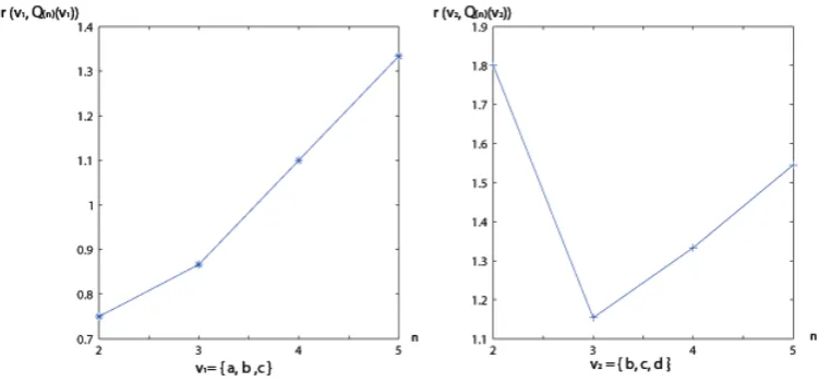
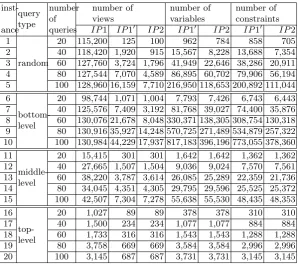
rmin({b, c, d}, Q) = 1.333. The values of the function r(v, Q(n)(v)) on different values of nfor v =v1 and for v =v2 are shown in Figure 2. We observe that
r(v1, Q(n)(v1))is an increasing function ofnfor2≤n≤5, andr(v2, Q(n)(v2)) decreases for2≤n≤3, and increases for 3≤n≤5.
Fig. 2.The minimum cost-benefit ratios in Example 1
the reduced search space contains at least one optimal solution. We discuss this subject in Section 4 below. Secondly, Observation 4 and Propositions 5 and 6 allow us to further reduce the search space of views by keeping only those views that are likely to be effective in answering the given collection of queries. This, in turns, allows us to solve larger instances of the problem, although we can no longer guarantee that the resulting solution is optimal for the original problem. We discuss this subject in Section 6.
4
Solving the problem
As mentioned earlier, Asgharzadeh et al. [3,4] employ the results stated in Obser-vations 1 and 2 in the context of a given problemDV S to remove certain views
from the search space, thus reducing the size of the corresponding IP modelIP1.
In this section we propose to further reduce the size of the IP model by employ-ing the results stated in Observation 3 and combinemploy-ing these results with those of Observations 1 and 2. Through a computational study in the next section we show empirical evidence of the effectiveness of this approach in solving relatively large instances of the problemDV S.
4.1 The reduction procedure
application. Thus, as we go through the collection of views in the setV in order to
identify the dominated views, for each view we test for the conditions stated in all three observations before moving to the next view. A detailed description of the reduction procedurethat we have devised to implement theses reductions is given below. The computational complexity of this procedure is O(|V|2) = O(4K),
whereK is the number of attributes in the database.
We use the binary representation of the subscript number for each view to indicate the set of attributes for the view. For instance, in a database with 4 attributesa,b,candd, the binary number “1001” represents the set of attributes
{a, d}. Hence, the subscript number of view{a, d}is 9 (= 23+ 20). We can now conduct the reductions on views by iterating over all the subscript numbers of the corresponding views inV. The pseudocode for this procedure is given in the
next page.
Algorithm 1The reduction procedure
Input: the given query setQand the search space of viewsV
Output: the reduced search space of viewsV
1: Sort the elements ofV in an increasing order of the subscript numbers 2: V ← ∅
3: fori←1to|V|do 4: v←ithelement ofV
5: f←1
6: a← | ∪q∈Q(v)q|
7: d(v, Q(v))←!q∈Q(v)S(q)−S(v)
8: if |v| %=aor(v%∈Qandd(v, Q(v))≤0)then
9: f←0
10: else
11: forj←1to|V|do 12: ˜v←jthelement ofV
13: if ˜v⊂vthen
14: if d(˜v, Q(˜v))≥d(v, Q(v))then
15: f←0
16: break
17: end if
18: end if
19: end for
20: end if 21: if f= 1then 22: V ←V ∪ {v}
23: end if 24: end for
In this procedure, we iterate through all the views in the view setV in the
increasing order of their subscript numbers, one view in each iteration (lines 1-4). Note that if a viewv answers a query (view)v", the subscript number ofv is
conducting the reductions regarding a view v, all the views that are subsets of v have already been considered in this procedure. The last view we consider in
this procedure is the raw-data view. In each iteration, we use a binary variable
f to indicate if viewv can be eliminate. At the beginning of each iteration, we
set f = 1 (line 5). In each iteration, we first conduct the reduction based on
Observations 1 and 2 (lines 6-9). More specifically, for each viewv, we compare
the number of attributes in v with that in the union set of the queries in Q
thatv can answer. We also compare the size of viewvwith the total size of the
queries inQthatv can answer. Note that the statements “|v| )=a” and “v)∈Q
and d(v, Q) ≤0” in line 8 indicate that v can be eliminated by the results of
Observation 1 and by the results of Observation 2, respectively. Then we conduct the reduction based on Observation 3 by iterating through each view ˜vthat has
been selected as a candidate view and can be answered by v (lines 11-19). For
each view ˜v, we compare the maximum benefit of v over Q (d(v, Q(v))) with
that of ˜voverQ(d(˜v, Q(˜v))). The statement “d(˜v, Q(˜v))≥d(v, Q(v))” indicates
the view v can be eliminated. At the end of each iteration, if the view is not
eliminated by any of the results of Observations 1-3, we add it into the view set
V (lines 21-23). At the beginning of the procedure, the view set V is an empty
set. As a result, at the end of this procedure,V is the new search space of views.
4.2 Smaller IP model
The structure of this model is similar to modelIP1 that we introduced in Section
2.2, except that we use the reduced search space of viewsV instead ofV. More
specifically, for each query qj ∈Q we define Vj ={vi ∈V :vi ⊇qj}. We also
define the associated sets of subscripts for V and Vj as I and Ij, respectively.
Using this notation we now define the smaller IP model that we refer to as model
IP2 as follows.
(IP2) minimize "
j∈J
"
i∈I
dijzij (15)
subject to "
i∈Ij
zij = 1 ∀j∈J (16)
zij ≤xi ∀j ∈J,∀i∈Ij (17)
"
i∈I
aixi≤b (18)
All variables are binary (19)
Based on the above observations, an optimal solution for modelIP2 is
guar-anteed to be optimal for IP1. Hence, it provides an optimal solution for the
original problem.
Obviously the size of model IP2 in terms of the number of variables and
the difference in size, however, depends on the specifies of each instance. In Section 5 we compare the sizes of these two models on an empirical basis and show that the difference in the sizes of the two models can be significant.
5
Experimental results with model
IP
2
In this section, we present the results of a computational experiment with the approach introduced in Section 4 for solving the problem DV S. Our objectives
are (i) examining the effectiveness of our approach in reducing the search space of views proposed in Section 4, and (ii) evaluating the scalability of the modelIP2
introduced in Section 4 and its effectiveness in solving relatively large instances of the problem DV S. We construct a collection of instances of the problem DV S with varying sizes using a number of datasets generated via the
TPC-H benchmark [24]. All of our algorithms are implemented in C++ and all the experiments are carried out on a 2.66GHz Intel 2 Quad processor with 3.25 GB RAM running Windows XP Professional. We use CPLEX 11 [16] to solve the integer programming models. We observe that the search spaces of views are significantly reduced inIP2 compared with modelsIP1 andIP1"introduced in
Sections 2.2, which, in turn, allows us to useIP2 to solve larger instances of the
problemDV S. More specifically, our experimental results show that:
– The search space of the views in modelIP2 is significantly smaller than that
of modelsIP1 andIP1". The magnitude of this difference depends on the
data set in each specific instance.
– Size of the model IP2, as measured by the number of variables and
con-straints, is sufficiently small to allow its use in solving relatively larger (realistic-size) instances of the problem within reasonable execution time. Of course, the resulting solution is guaranteed to be optimal for the original problemDV S.
– In some larger (realistic-size) instances of problemDV S, however, the size
of the corresponding model IP2 is too large for current “state of art” IP
solver. In the next section we propose alternative (scalable) approaches for solving such (larger) instances of the problem.
5.1 Constructing the instances
The input parameters for an instance of the problemDV S are a databaseD, a query setQ, and the space limitb. In this section, we use two different datasets
based on the TPC-H benchmark [24] – a 13-attribute dataset, and a 17-attribute dataset – to construct the collection of instances in our experiments. The same datasets are used in [3–5].
For each instance we generate the queries in the query set randomly. More specifically, given a database fact table (that is, stored relation) D withK
at-tributes, and given two integerst0and t1∈[1, K−1], we construct each query
construct such a query q, we first determine the number of attributes in q by
randomly generating an integertbetweent0 andt1. Then, we randomly choose
t distinct integers a1, . . . , at from {1,2, . . . , K} as the attributes of q. Then,
{a1, . . . , at}uniquely defines queryqover the database D.
Our preliminary experiments showed that the computational requirements of solving model IP2 in each instance depend on the relative magnitude of the
storage space limits as compared with the size of the queries. In this section for all instances based on the TPC-H datasets we choose the storage space limit
b equal to one fifth of the sum of the sizes of the queries in Q, that is b =
0.2∗#q∈QS(q). Our empirical observations show that typically at this value of b the computational requirements of solving the model IP2 are relatively high
as compared with these requirements at other values ofb.
5.2 Reduction in the size of search space
We compare the size of the models IP1, IP1" and IP2 for several randomly
generated instances of the problem DV S. More specifically, we constructed 20
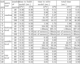
instances for the 13-attribute TPC-H dataset in such a way that for each instance the number of attribute of each query is a random number between 1 and 12. (These queries are randomly chosen from the entire view lattice.) The number of queries for each instance ranges from 20 to 100. We also construct 20 instances for the 17-attribute TPC-H dataset. For the instances 1 to 5 in this group, the number of attributes of each query is a random number between 1 and 16, (that is, each query is chosen from the entire view lattice). For the each of the remaining instances, all of the queries are from certain levels of the view lattice. For the instances 6 to 10, the number of attributes in each query is a random number between 1 and 8, (that is, each query is chosen from the bottom levels of the view lattice). For the instances 11 to 15, the number of attributes of each query is a random number between 5 and 12, (that is, each query is chosen from the middle levels of the view lattice). Finally for the instances 16 to 20, the number of attributes of each query is a random number between 9 and 16, (that is, each query is chosen from the top levels of the view lattice). We refer to the query types of those instances as “bottom-level”, “middle-level”, and “top-level”, respectively. Within the collection of instances for each query type, the number of queries ranges from 20 to 100. For each instance, we report the number of views in modelsIP1,IP1" andIP2. For the 20 instances on the
17-attribute dataset, these values are in Table 1. For each instance, we also report the number of variables and constraints in each model. (We do not construct model IP1 since [4] has already shown thatIP1" is much more effective than IP1.) In Table 2 we report the corresponding execution times. More specifically
Table 1. Comparison of the number of views and the sizes in the modelsIP1,IP1"
andIP2, for instances over the 17-attribute TPC-H dataset
inst-ance query type
number of queries
number of views
number of variables
number of constraints
IP1 IP1" IP2 IP1" IP2 IP1" IP2
1
random
20 115,200 125 100 962 784 858 705
2 40 118,420 1,920 915 15,567 8,228 13,688 7,354
3 60 127,760 3,724 1,796 41,949 22,646 38,286 20,911 4 80 127,544 7,070 4,589 86,895 60,702 79,906 56,194 5 100 128,960 16,159 7,710 216,950 118,653 200,892 111,044 6
bottom-level
20 98,744 1,071 1,004 7,793 7,426 6,743 6,443 7 40 125,576 7,409 3,192 81,768 39,027 74,400 35,876 8 60 130,076 21,678 8,048 330,371 138,305 308,754 130,318 9 80 130,916 35,927 14,248 570,725 271,489 534,879 257,322 10 100 130,984 44,229 17,937 817,183 396,196 773,055 378,360 11
middle-level
20 15,415 301 301 1,642 1,642 1,362 1,362
12 40 27,665 1,507 1,504 9,036 9,024 7,570 7,561
13 60 38,220 3,787 3,614 26,085 25,289 22,359 21,736 14 80 34,045 4,351 4,305 29,795 29,596 25,525 25,372 15 100 42,507 7,304 7,278 55,638 55,530 48,435 48,353 16
top-level
20 1,027 89 89 378 378 310 310
17 40 1,500 234 234 1,077 1,077 884 884
18 60 1,733 316 316 1,543 1,543 1,288 1,288
19 80 3,758 669 669 3,584 3,584 2,996 2,996
Table 2.Comparison of the computing times of the modelsIP1"andIP2, for instances over the 17-attribute TPC-H dataset
inst-ance query type
number of queries
time to build model (sec.)
time to solve model (sec.)
total time (sec.)
IP1" IP2 IP1" IP2 IP1" IP2
1
random
20 0.30 0.30 0.14 0.11 0.44 0.41
2 40 0.41 0.39 2.86 1.56 3.27 1.95
3 60 0.66 0.64 7.47 3.47 8.13 4.11
4 80 0.81 1.13 31.77 17.17 32.58 18.30
5 100 1.33 2.05 116.05 44.15 117.38 46.20
6
bottom-level
20 0.41 0.50 1.58 1.72 1.99 2.22
7 40 0.70 0.80 104.28 32.53 104.98 33.33
8 60 1.56 2.28 >30min 385.14 >30min 387.42
9 80 3.19 6.19 out of memory>30min out of memory>30min 10 100 3.11 9.42 out of memory>30min out of memory>30min 11
middle-level
20 0.25 0.25 0.42 0.42 0.67 0.67
12 40 0.31 0.34 4.44 3.89 4.75 4.23
13 60 0.45 0.67 22.42 21.05 22.87 21.72
14 80 0.52 0.80 103.19 93.26 103.71 94.06
15 100 0.61 1.39 >30min>30min >30min>30min 16
top-level
20 0.25 0.22 0.11 0.05 0.36 0.27
17 40 0.30 0.27 2.56 2.28 2.86 2.55
18 60 0.31 0.33 1.08 1.06 1.39 1.39
19 80 0.34 0.38 1.63 1.62 1.97 2.00
1. In every instance the number of views in the search space for models IP1"
andIP2 are significantly smaller than the corresponding number in model IP1. This reduction is relatively more significant for the instances with a
small ratio of the number of queries over the total number of views in the dataset. More specifically, when we have a larger number of queries, the ratio of the number of queries over the total number of views increases (since the total number of views for a 17-attribute dataset is constant and equal to 131072), and the magnitude of associated reductions in the number of views in the search space decreases. We make a similar observation on the instances over the 13-attribute dataset.
2. Comparing the number of views in IP1" and IP2, we note that for the
instances where the queries are from the entire view lattice (instances 1 to 5) or from the bottom levels of the view lattice (instances 6 to 10), the size of IP2 is significantly smaller than that of IP1". It is also observed that
for these instances the size ofIP2, when expressed by the total number of
variables and constraints, is much smaller than that ofIP1". In addition,
the time to solveIP2 is also significantly smaller than that for IP1". On
the other hand, for the instances where the queries are from the middle levels of the view lattice (instances 11 to 15) the reduction in the number of views in the search space from model IP1" to IP2 is not as significant,
resulting in no significant difference in the size and the solving time between the corresponding modelsIP1" andIP2. Moreover, for the instances from
the top levels of the view lattice (instances 16 to 20), we observe no reduction in the number of views in the search space from modelIP1" toIP2. These
observations are consistent with our expectations as evident from the nature of Observation 3.
3. It is observed that for all instances the time to build the model IP2 is
relatively larger than that for IP1". This increase in time is much more
significant for instances with large number of queries. Comparing the time to build and the time to solve the modelsIP1"andIP2, however, we observe
that the decrease in the time to solve the modelIP2 compared with model IP1" is much more significant than the increase in the time to build the
model IP2 compared with model IP1". In general it is also observed that
the total time forIP2 is relatively smaller than that forIP1". This reduction
in time is more significant for instances where the queries are from the entire view lattice (instances 1 to 5) or from the bottom levels of the view lattice (instances 6 to 10).
5.3 Scalability of the model IP2
In order to evaluate the scalability of our approach we attempt to solve larger instances of the problemDV S by modelIP2.
In Table 2 we observe that for instances 6 to 10, where the queries are from the bottom levels of the view lattice, the total execution time to solveIP2 ranges
is no more than 60. However, we could not solve instances 9 and 10 within the assumed time limit 30 minutes.
As reported in Table 2 for instances 11 to 15 where queries are from the middle levels of the view lattice over the 17-attribute dataset, we observe that we could solve all the instances whose number of queries is no more than 80. The total execution time for IP2 ranges from 0.67 seconds to 94.06 seconds.
However, when we increase the size of the query set further to 100, the solver fails to provide an optimal solution for model IP2 within our time limit of 30
minutes.
For instances where the queries are from the entire view lattice over the 17-attribute dataset (instances 1 to 5) that we report in Table 2, we note that the total execution time for the model IP2 ranges from 0.41 seconds to 46.20
seconds. We also note that this time increases as we increase the number of queries in the query set.
In addition, as observed in Table 2 we could solve within 5 seconds all the instances where the queries are from the top levels of the view lattice over the 17-attribute dataset (instances 16 to 20).
In order to further observe the execution time for solving larger instances of the problem where queries are from the entire view lattice, and for instances where queries are from top levels of the lattice, we constructed several instances with even larger number of queries over the 17-attribute dataset as reported in Table 3. Note that for these instances we do not construct the correspond-ing modelIP1", since we have already observed that modelIP2 is much more
effective than modelIP1" for these types of instances.
Table 3.Scalability ofIP2 for instances over the 17-attribute TPC-H dataset
ins-tance
query type
number of queries
number of views
time to build
IP2 (sec.)
time to solve
IP2 (sec.)
total time (sec.) 21
random
220 23256 13.00 304.00 317.00
22 240 23921 14.25 374.22 388.47
23 260 25922 15.31 out of memory out of memory
24 top-level
320 2673 0.91 559.58 560.49
25 340 2703 1.08 814.27 815.35
26 360 2930 1.20 >30min >30min
6
Heuristic methods
As stated earlier, Observation 4 and Propositions 5-6 allow us to further reduce the size of the search space of views by keeping only those views that are likely to be effective in answering the given collection of queries in the context of the problem DV S. In this section we propose several strategies for carrying
out this task, leading to two distinct procedures that we refer to as heuristic methods I and II, respectively. We start the section by discussing the relationship between the cost-benefit ratio and the modelIP2. Subsequently, we build on the
discussion to derive two distinct heuristic methods for reducing the search space of views and the size of the corresponding IP model.
6.1 Cost-benefit ratio and the model IP2
In this subsection, we discuss the relationship between the cost-benefit ratio and the integer programming modelIP2, and provide an intuitive justification as to
why a view with relatively low cost-benefit ratio is more favorable to be selected in the context of the problemDV S.
We denote byJ(v) the set of subscripts for the queries inQ(v). As introduced
in Section 2.1, if viewvican answer queryqj, then the cost of answeringqj using
vi is the size of vi. Equivalently, we have that dij =ai =S(vi). We now show
that the objective function of the model IP2 can be interpreted as the sum of
theextra costs of answering the queries using the materialized views instead of the queries themselves, as defined in Equation 8, plus a constant. To this end, we rewrite the objective function (15) ofIP2 as follows.
"
j∈J
"
i∈Ij
dijzij =
"
j∈J
"
i∈Ij
S(vi)zij (20)
="
j∈J
"
i∈Ij
S(vi)zij−
"
j∈J
S(qj) +
"
j∈J
S(qj) (21)
="
j∈J
"
i∈Ij
S(vi)zij−
"
j∈J
S(qj)
"
i∈Ij
zij+
"
j∈J
S(qj) (22)
="
j∈J
"
i∈Ij
zij
)
S(vi)−S(qj)
*
+"
j∈J
S(qj) (23)
="
i∈I
xi
+ "
j∈J(vi)
zij
)
S(vi)−S(qj)
*,
+"
j∈J
S(qj) (24)
For each view vi, we define the extra cost of using view vi to answer query
qj ∈ Q(vi) as
)
S(vi)−S(qj)
*
. Using the binary variables zij as defined in
the IP model, it follows that #j∈J(vi)zij
)
S(vi)−S(qj)
*